Functional Network Stability and Average Minimal Distance – A ...

Accepted Manuscript Title: Functional Network Stability and Average Minimal Distance – A framework to rapidly assess dynamics of functional network representations Authors: Jiaxing Wu, Quinton M. Skilling, Daniel Maruyama, Chenguang Li, Nicolette Ognjanovski, Sara Aton, Michal Zochowski PII: DOI: Reference:

S0165-0270(17)30439-9 https://doi.org/10.1016/j.jneumeth.2017.12.021 NSM 7927

To appear in:

Journal of Neuroscience Methods

Received date: Revised date: Accepted date:

24-8-2017 21-12-2017 24-12-2017

Please cite this article as: Wu Jiaxing, Skilling Quinton M, Maruyama Daniel, Li Chenguang, Ognjanovski Nicolette, Aton Sara, Zochowski Michal.Functional Network Stability and Average Minimal Distance – A framework to rapidly assess dynamics of functional network representations.Journal of Neuroscience Methods https://doi.org/10.1016/j.jneumeth.2017.12.021 This is a PDF file of an unedited manuscript that has been accepted for publication. As a service to our customers we are providing this early version of the manuscript. The manuscript will undergo copyediting, typesetting, and review of the resulting proof before it is published in its final form. Please note that during the production process errors may be discovered which could affect the content, and all legal disclaimers that apply to the journal pertain.

Title: Functional Network Stability and Average Minimal Distance – A framework to rapidly assess dynamics of functional network representations

SC RI PT

Contributing Authors and Affiliations: Jiaxing Wu*,1, Quinton M Skilling*,2, Daniel Maruyama*,3, Chenguang Li4, Nicolette Ognjanovski5, Sara Aton5, Michal Zochowski1, 2, 3 1

Applied Physics Program, 2Biophysics Program, 3Department of Physics, 4R.E.U program in Biophysics, 5Department of Molecular, Cellular, and Developmental Biology, University of Michigan, Ann Arbor, Michigan, USA 48109 * These authors contributed equally to the manuscript. *

N

Number of Pages: 31 pages, including title page, figures, and references

M

A

Figures: 16 Figures Tables: 1 Table

D

Highlights

TE

A framework to rapidly detect dynamics of functional network states. It captures functional connectivity patterns more effectively than other methods. Functional similarity metric measures global network response to local changes. It bridges the gap between time scales of neural activity and behavioral states.

A

CC

EP

   

U

Corresponding Author: Michal Zochowski,n , University of Michigan, Randall Lab, 450 Church Street, Ann Arbor, MI 48109-1040, Email: [email protected]

Abstract: Background Recent advances in neurophysiological recording techniques have increased both the spatial and temporal resolution of data. New methodologies are required that can handle large data sets in an efficient manner as well as to make quantifiable, and realistic, predictions about the global modality of the brain from under-sampled recordings. New Method 1

M

A

N

U

SC RI PT

To rectify both problems, we first propose an analytical modification to an existing functional connectivity algorithm, Average Minimal Distance (AMD), to rapidly capture functional network connectivity. We then complement this algorithm by introducing Functional Network Stability (FuNS), a metric that can be used to quickly assess the global network dynamic changes over time, without being constrained by the activities of a specific set of neurons. Results We systematically test the performance of AMD and FuNS (1) on artificial spiking data with different statistical characteristics, (2) from spiking data generated using a neural network model, and (3) using in vivo data recorded from mouse hippocampus during fear learning. Our results show that AMD and FuNS are able to monitor the change in network dynamics during memory consolidation. Comparison with other methods AMD outperforms traditional bootstrapping and cross-correlation (CC) methods in both significance and computation time. Simultaneously, FuNS provides a reliable way to establish a link between local structural network changes, global dynamics of network-wide representations activity, and behavior. Conclusions The AMD-FuNS framework should be universally useful in linking long time-scale, global network dynamics and cognitive behavior. Key words: Functional connectivity structure, network dynamics, functional stability

Key Words

TE

Introduction

D

Functional connectivity, network dynamics, functional stability, learning, excitatory/inhibitory balance

A

CC

EP

New multisite recording techniques have generated a wealth of data on neuronal activity patterns in various brain modalities (Buzsaki, 2004; Lichtman et al., 2008; Luo et al., 2008; Chorev et al., 2009). An unresolved question is how, using such data sets, one can correctly identify largescale network dynamics from populations of neurons which either may, or may not, include neurons involved in a particular cognitive process of interest. This is due in part to the fact that even high-density recordings sample only a sparse subset of the neural system responsible for the modality in question. It is also complicated by the inherent separation of temporal scales over which neural vs. behavioral measurements occur. In response to this question, multiple linear and non-linear techniques have been developed over the years to assess functional connectivity between neurons, and to possibly infer from it structural connectivity (see for example: Friston et al., 2013; Bastos and Schoffelen, 2016; Cimenser et al., 2011; Cestnik and Rosenblum, 2017; Zaytsev et al., 2015; Poli et al., 2016; Shen et al., 2015; Wang et al., 2014). More recent approaches utilize network theory to establish links between recorded data and the underlying connectivity (see for example: Newman, 2004, 2006, 2010; Ponten et al., 2010; Rubinov and Sporns, 2010; Sporns et al., 2000; De Vico Fallani et al. 2014; Supekar et al., 2008; Boccaletti et al., 2006; Stafford et al., 2014; Petersen and Sporns, 2015; Misic and Sporns, 2016; Park and Friston, 2013; Bassett et al., 2010; Feldt et al., 2011; Gu et al., 2015; Medaglia et al., 2017; Davison et al., 2015; Hermundstad et al., 2011; Bassett, et al., 2011; 2

A

CC

EP

TE

D

M

A

N

U

SC RI PT

Shimono and Beggs, 2015; Nigam et al., 2016; Nakhnikian et al., 2014; Pajevic and Plenz, 2009). The idea is that, by estimating networks based on functional interactions, one can potentially gain insight into global dynamics, which reflect the general property of the whole network, instead of a specific subset of neurons. While all these approaches can provide insightful information, they share some the same problems. These methods are often limited by under-sampling (and potentially unrepresentative sampling) of neuronal recordings, and are not optimized for monitoring changes in network structure across extended time periods (i.e., those associated with behaviors of interest, such as memory formation). Here we propose a novel technique that rapidly estimates functional connectivity between recorded neurons. Then, rather than characterizing details of the recovered network, the metric measures changes in the network dynamical stability over time. The technique is based on an estimation of Average Minimal Distance (AMD) between spike trains of recorded neurons, a metric which has previously been compared to other clustering algorithms (Feldt et al., 2009). Here, we expand on this work and show that the analytic estimation of AMD for the null case, when the two cells are independent, allows for rapid estimation of the significance of pairwise connections between the spike trains, without need for time-expensive bootstrapping. Further, Functional Network Stability (FuNS) is introduced and is monitored over timescales relevant for behavior. We show that FuNS measures global change in network dynamics in response to localized changes within the network. This, in part, alleviates the problem of sparse sampling so prevalent in neuroscience. Below, the statistical underpinnings of AMD and FuNS are detailed. We compare AMD and cross-correlation (CC) on both surrogate data and model simulation data. Model results show the applicability of AMD and FuNS on excitatory-only networks, as well as on mixed networks of excitatory and inhibitory neurons poised near a balance between excitation and inhibition, a regime thought to be a universal dynamical state achieved by brain networks, resulting in enhanced information processing properties (Froemke, 2015; Barral and Reyes, 2016; Poil et al., 2012; Berg et al., 2007; Rubin et al., 2017). We end by analyzing experimental data recorded from the mouse hippocampus during contextual fear memory formation. Our results indicate that AMD yields results comparable to that of the gold-standard CC, but, importantly, it is orders of magnitude faster and reports statistically significant increases in FuNS due to behavioral-based network topological changes compared to CC FuNS.

Table 1: List of Common Abbreviations

Abbreviation

Full Name

3

Average Minimal Distance

CA1

Cornu Ammonis 1

CC

Cross-correlation

CFC

Contextual Fear Conditioning

E/I

Excitatory/Inhibitory Ratio

FC

Functional Connectivity

FCM

Functional Connectivity Matrix

FSM

Functional Stability Matrix

FuNS

Functional Network Stability

IAF

Integrate and fire

ISI

Interspike interval

SC RI PT

AMD

Methods 1. Statistical methods

U

1.1.Average minimal distance (AMD) and its significance estimation

M

A

N

Pairwise functional connectivity is estimated using average minimal distance (AMD) (Feldt et al., 2009) (Figure 1) separating the relative spike times between neurons. AMD is calculated as follows: given the full spike trains {S1, S2, …, Sn} for n neurons within a network, the pairwise functional relationship, FCij, of the ith and jth neurons is evaluated by comparing the average temporal closeness of spike trains Si and Sj to the expected sampling distance of train Sj (Figure 1a). That is, 𝟏 𝑨𝑴𝑫𝒊𝒋 = 𝑵 ∑𝒌 ∆𝒕𝒊𝒌 , where Ni is the number of events in Si and ∆𝒕𝒊𝒌 is the temporal distance 𝒊

A

CC

EP

TE

D

between an event k in Si to the nearest event in Sj. With AMD measured, the functional connectivity (FC) is calculated as 𝑭𝑪𝒊𝒋 = √𝑵𝒊 ∗ (𝑨𝑴𝑫𝒊𝒋 − 𝝁𝒋 )⁄𝝈𝒋 , which is expressed in terms of probabilistic significance of connectivity between pair ij. The mean and standard deviation, μ j and σj, of the expected sampling distance, assuming that the spike trains are independent, can be calculated from either: 1) boot-strapping (i.e. randomizing the spike trains multiple times and reassessing the AMD for the null hypothesis being statistically independent of the two spike trains), or 2) numerical estimation of expected values given the distribution of inter-spike intervals (ISIs) on Sj. Hereafter, the analytical method is referred to as “fast AMD” and the bootstrapping method as “bootstrapped AMD”. For a system with n neurons, the functional connectivity value between each pair of spike trains is calculated, generating an n-by-n Functional Connectivity Matrix (FCM).

4

In the fast AMD approach, the maximal distance between an input spike and any spike in 𝑰𝑺𝑰 the spike train to be analyzed is 𝟐 𝒊. Then, the expected mean distance between spikes in the 𝑰𝑺𝑰

D

M

A

N

U

SC RI PT

independent spike trains is 𝝁𝒊 = 𝟒 𝒊 , where ISIi is the corresponding interspike interval of spike train i (Figure 1b). Calculating the first and second raw moments from the maximal distance then 𝟏 𝟏 yields 𝝁𝑳𝟏 = 𝟒 𝑳 and 𝝁𝑳𝟐 = 𝟏𝟐 𝑳𝟐 for a specific ISI with length L. Taking into account the probability

EP

TE

Figure 1. Calculation of AMD and analytical significance. The average minimal distance algorithm calculates shortest temporal length between spikes emitted by a neuron to the closest spikes in a reference neuron, looking in either both temporal directions (a), or in a single temporal direction (b), e.g. forward in time. The maximal possible distance between spikes is either half the interspike interval (c) or the full interspike interval (d), when looking in either both temporal directions or a single temporal direction, respectively. The measurements require a collective average timing sequence to be below one quarter (bidirectional) or one half the interspike interval (unidirectional) in order to be considered significant.

CC

of observing an ISI with length L over the recording interval T, 𝒑(𝑳) = moment for sampling the whole spike train randomly are then 𝝁𝟏 = 𝑳

𝟏

𝑳

, the first and second

𝑻 𝑳 𝑳 𝟏 ∑𝑳 𝝁 𝟏 = ∑𝑳 𝑳 𝟐 𝑻 𝟒𝑻

and 𝝁𝟐 =

A

∑𝑳 𝝁𝑳𝟐 = ∑ 𝑳𝟑 , respectively. The expected mean and standard deviation of a random spike 𝑻 𝟏𝟐𝑻 𝑳 train are then calculated as 𝝁 = 𝝁𝟏 and 𝝈 = √𝝁𝟐 − 𝝁𝟐𝟏 . 1.2. Unidirectional AMD for causality detection:

The bidirectional AMD described above (i.e. the temporal distance between spikes of two different neurons, measured in either direction) can be extended to be unidirectional to identify causality between the two spike trains. In this scenario, the temporal distance is measured only 5

forward in time and the mean delay time expected within the null hypothesis (i.e. independence of 𝑰𝑺𝑰 both spike trains) is only set to 𝝁𝒊 = 𝟐 𝒊 , assuming a maximal temporal distance equal to the ISI (Figure 1c and 1d). The calculation of first and second moment change accordingly to 𝝁𝟏 = 𝟏 𝟏 ∑𝑳 𝑳𝟐 and 𝝁𝟐 = ∑𝑳 𝑳𝟑 ; the mean and standard are then calculated in the same manner as 𝟐𝑻 𝟑𝑻 above.

SC RI PT

1.3. Functional Stability Matrices (FSMs) and functional network stability (FuNS)



, with an absolute value of 1 denoting no change (maximum

√∗

D

𝒄𝒐𝒔 𝜽𝑨𝑩 =

M

A

N

U

The fast AMD metric offers critical advantage over the bootstrapped AMD method, as well as over the standard CC method, for quantifying functional connectivity measured over behaviorally-relevant timescales (i.e., hours to days). It allows rapid analysis of functional connectivity that can then be used to link neuronal activity with behavior. The speed of the fast AMD metric is utilized to introduce Functional network stability (FuNS) as a way of measuring the dynamics of functional connectivity over time. Namely, we want to assess the stability of functional connectivity between the neurons within the network rather than to characterize the detailed network connectivity, which, again, is usually based on extremely sub-sampled systems. The remainder of this section is focused on characterizing the stability metric. Later, we show that changes in stability provide information about gross structural changes in the network. Calculating the stability of network-wide functional connectivity patterns across time requires a division of the data sets into at least two time-windows; the remaining theoretical discussion assumes two time-windows for simplicity. The functional connectivity matrices are denoted as FA and FB where A and B represent the first and second time windows, respectively. The functional stability between these data sets is then calculated using cosine similarity, 𝑪𝑨,𝑩 =

A

CC

EP

TE

similarity) and 0 indicating great change (no similarity; orthogonality) between the time intervals (Figure 2a). Functional stability can thus be calculated in a pairwise manner across all time bins for a given recording in order to generate what we call a functional stability matrix (FSM; Figure 2b, see also Figure 8), or only on directly-adjacent time windows (Figure 2a), to generate a single 𝟏 measure of stability: 𝑭𝒖𝑵𝑺 = 𝑻 ∑𝑻−𝟏 𝒕=𝟎 𝑪𝒕,𝒕+𝟏 .

6

SC RI PT U

M

A

N

Figure 2. Calculation of Functional Network Stability and Construction of Functional Stability Matrices. a) Given the spike time series of neurons (top), the functional connectivity matrices (FCMs) are calculated over each interval (center), whereupon FuNS is calculated by measuring the mean cosine similarity between each consecutive time interval (bottom). b) Alternatively, similarity can be calculated in a pairwise manner across all time intervals to yield the functional stability matrix (FSM).

TE

D

FuNS can also be used to determine the effect behavior has on neural network dynamics. In this scenario, stability is calculated before and after the presence of a synaptic heterogeneity (see Methods 2.2), 𝑭𝒖𝑵𝑺𝑨,𝑩 and 𝑭𝒖𝑵𝑺𝑪,𝑫, respectively. The significance of stability increase over many simulations is then given as a Z-score: 𝒁𝒔 = (𝝁𝑪,𝑫 − 𝝁𝑨,𝑩 ) (

𝝈𝟐𝑨,𝑩 𝑵

+

𝝈𝟐𝑪,𝑫 𝑵

−𝟏𝟐

)

with values

EP

greater than 2 indicating a significant increase in stability due to behavioral effects and values less than -2 indicating a significant decrease in stability. Here, μ and σ represent the mean and standard deviation of functional network stability, respectively, taken over many simulations or recordings.

CC

2. Computer simulations

A

2.1.Simulations of integrate and fire networks Neural activity is simulated using leaky integrate-and-fire model neurons with dynamics given by 𝑽̇ = −𝜶𝑽 + ∑𝒋 𝝎𝒊𝒋 𝑿𝒋 + 𝑰𝝃 . The summation represents the total input from recently fired (within ~20ms) pre-synaptic neurons with connectivity strength 𝝎𝒊𝒋 and input dynamics given by the double exponential 𝒔𝒑𝒌

𝒔𝒑𝒌

𝒔𝒑𝒌

𝑿𝒋 = 𝒆𝒙𝒑(−(𝒕 − 𝒕𝒋 )/𝟑. 𝟎) − 𝒆𝒙𝒑(−(𝒕 − 𝒕𝒋 )/𝟎. 𝟑), where 𝒕𝒋 last pre-synaptic spike.

7

represents the timing of the

N

U

SC RI PT

In addition to synaptic input, each neuron receives noisy input 𝑰𝝃 = 𝟎. 𝟏𝟓 + 𝟏𝟎𝑯(𝝃 − 𝒑), where H is the Heaviside step function, 𝝃 = 𝟏𝟎−𝟓 , and 𝒑 ∈ {[𝟎, 𝟏]} is real-valued, random variable generated at every integration step from a uniform distribution. Networks are formed using 1000 excitatory neurons arranged on a ring network. Connection densities range from 1.5% to 4.5% of the network population and connection weights range from ω = 0.02 to ω = 0.045 unless stated otherwise. The networks are initially connected locally and subsequently rewired with probability pr. This parameter is varied from zero to unity, changing network topology from completely local connections to completely random. Each simulation is completed using the Euler integration method. Additional network are simulated using a mixed population of excitatory/inhibitory cells. In this scenario, connections are completely local (𝒑𝒓 = 𝟎), have a connection density of 2%, and synaptic weights are pulled from a uniform distribution 𝝎𝒋𝒊 ∈ {[𝟎, 𝟎. 𝟐]}. These networks follow the same dynamics as the excitatory only networks, except that 225 inhibitory neurons are added to the existing networks, evenly spaced among the excitatory cells, with inhibitory output connectivity strength 𝝎∗𝒋𝒊 = −𝜷𝝎𝒋𝒊. The variable 𝜷 is used to investigate network dynamics when excitation or inhibition dominate. We calculate the ratio of excitation to inhibition, E/I, as the ratio between total excitatory to inhibitory synaptic input, averaged over all neurons not in the heterogeneity. Balance between excitation and inhibition (E/I ~ 1) occurs at 𝜷 = 𝟑. 𝟎.

A

2.2.Introduction of synaptic heterogeneities and their long-range dynamical effects

A

CC

EP

TE

D

M

Sensory input causes topological changes in anatomical network structure through both the strengthening and weakening of synapses (Feldman, 2012; Song et al., 2000) as well as through the introduction of new synapses (Ghiani et al., 2007) and depletion of unused synapses (Vanderhaeghen and Cheng, 2010). Here, we focus solely on the strengthening of synaptic coupling for simplicity. The effect of synaptic strengthening is mimicked by introducing a discrete heterogeneity in network connectivity, i.e. a small, localized region spanning 10% of the network, with increased synaptic connectivity between nodes. To simplify comparing networks with and without these synaptic heterogeneities, the underlying pairwise connectivity and synaptic strengths are conserved. To analyze the potential long-range effects of such a heterogeneity, we calculate the mean synaptic distance to the heterogeneity for each neuron not in the heterogeneity. The mean synaptic distance here is the average number of steps that need to be taken from neurons in the heterogeneity to any other neuron in the network, along synaptic connections. The calculation of the distance is adopted from Newman (2010). In the simplest way, the synaptic distance between every neuron can be measured by calculating AN, where A is the adjacency matrix and the power N is the number of synaptic steps necessary to reach every other neuron. With each successive multiplication of A, new non-zeros entries appear, representing new long-range (i.e. not directly connected), multi-unit synaptic connections. The synaptic distance d is the number of multiplications of A with itself, necessary to give rise to the new long-range connection. With the full synaptic distance matrix populated, the mean synaptic distance to the heterogeneity is calculated by averaging over all heterogeneity distances calculated for a given neuron. The mean synaptic distance to heterogeneity, and indeed between any two neurons, changes based on the size and connectivity density of the network. We thus normalize the distance to heterogeneity with a value of 1 representing neurons farthest from the heterogeneity, incorporating the entire network, and a value 8

of 0 representing the minimum degree of separation from the heterogeneity (i.e. within the heterogeneity). It should be noted that by definition of d, the shortest distance to heterogeneity would be for a neuron not in the heterogeneity but connected to every other neuron within the 𝟏 heterogeneity, attaining a normalized value of = 𝑵 .

3. Experimental design

SC RI PT

3.1.Recordings from mouse CA1 before and after contextual fear conditioning (CFC)

U

To test the effects of memory formation on network dynamics in vivo, C57BL/6J mice (age 1-4 months) were implanted with custom-built driveable headstages (see Ognjanovski et al., 2014, 2017) with bundles of stereotrodes targeting hippocampal area CA1. Following postoperative recovery, mice were handled daily while gradually lowering stereotrodes into the pyramidal cell layer of CA1 to obtain stable recordings. A 24-h baseline recording of neuronal and LFP activity was initiated at CT0, after which mice underwent a single-trial CFC as described previously. Contextual fear memory was assessed 24 h after CFC, using previously-described methods.

1. Comparing AMD and CC in surrogate data

N

Results

A

1.1 Comparison of bootstrapped AMD, fast AMD, and CC for rapid estimation of functional connectivity.

A

CC

EP

TE

D

M

We first compare the bootstrapped and fast AMD metrics for different distributions of ISIs (Figure 3): Gaussian, Poisson, uniform, and exponential. To measure the performance of the metrics, a single spike train following any one of these distributions is generated and cloned, with clones receiving a bidirectional jitter of their spike times equal to the jitter width depicted on the x axis (Figure 3). The jitter from every spike is drawn from the same distribution as the original spike train, of which the standard deviation serves as the jitter width. For all cases, the mean ISI is arbitrarily chosen to be ~33ms (this ISI gives a 30Hz signal, representative of awake brain oscillations). Figure 3 depicts the mean z-score and its standard deviation, calculated as a function of the jitter width for the two approaches. In all four instances, the two AMD methods perform nearly identically. Next, we compare the performance of fast AMD to CC, using the same distributions as above, i.e. Gaussian, Poisson, etc., with jittering (Figure 4). To calculate CC between two spike trains, the two spike trains are convolved with a Gaussian having one of three different widths,  = 1ms, 5ms, or 33ms. Both metrics are calculated for 0 temporal shift between the spike trains. Importantly, we note that AMD does not have any free parameters and, at the same time, better captures finer characteristics for Poisson spike distributions compared to CC with any Gaussian convolution width. Critically, the fast AMD approach provides a rapid estimation of the significance of pairwise functional connectivity. Figure 5 shows the computing times of fast AMD, bootstrapped AMD, and CC with zero time-shift and bootstrapping for spike trains having various numbers of spikes and network sizes. The reduction of the computing time for fast AMD is very significant (up to 10000 times faster) which may be crucial for multiscale data analysis.

9

SC RI PT U N A

A

CC

EP

TE

D

M

Figure 3. Comparison of bootstrapped and fast AMD metrics for rapid estimation of functional connectivity (FC). Two identical spike trains were artificially generated using various distributions of inter-spike intervals: a) Gaussian, b) Poisson, c) uniform, and d) exponential; the second spike train was jittered using the same type of statistical distribution, with various jitter widths (x-axis) to progressively de-correlate the spike trains. Each set of spiking data represents a 1s long recording (the time length is arbitrary, however all values are scaled to length) and contains 30 spikes. The analytical value of pairwise functional connectivity (𝑭𝑪𝟐𝟏 ) is calculated using the method described in the text (Methods 1.1). For all the distributions, AMD detects the significant functional connectivity when jitter width is small. The average value at which FC loses significance is a quarter of mean ISI, ~ 8ms. For a Poisson distribution (b), due to the fact that the mean value and standard deviation are controlled by the same parameter, when the jitter width equals around 17ms, the mean value of jitter is also around 17ms, and the maximal value of the AMD and therefore FC has the most negative value. The same reasoning applies when the jitter width is around 33ms. The significance from bootstrapping was obtained by shuffling the ISIs of the second train 100 times. As before, the Z-score of the AMD values represents the FC. The results agree with the analytical values.

10

SC RI PT U N A

A

CC

EP

TE

D

M

Figure 4. Comparison between fast AMD and CC. We compared the traditional cross-correlation (CC) method to fast AMD using a) Gaussian, b) Poisson, c) uniform, and d) exponential distributions, as in Figure 3. For the CC calculation, spike trains are convolved with a Gaussian waveform having a standard deviation σ as a free parameter. We used sigma σ = 1ms, 5ms and 33ms respectively. As before, the Z-score of CC was based on bootstrapping. AMD and CC results are equivalent for σ = 1ms. For larger σ, CC cannot capture the specific features of ISIs distributions, but behaves generally in a similar manner as AMD for increasing jitter width.

11

SC RI PT

TE

D

M

A

N

U

Figure 5. Comparison of computation speeds obtained for fast AMD, bootstrapped AMD, and bootstrapped CC. We measured the calculation time (recorded by CPU time from MATLAB) for three methods: CC, bootstrapped AMD and fast AMD. a) Calculation time for increasing the number of cells in the system. B) Calculation time for increasing the number of spikes in a two-cell system. Fast AMD is more than 20 times faster than bootstrapped AMD, and 200 times faster than CC calculation. For two-cell systems with different number of spikes (b), the advantage of fast AMD is more significant for larger spike trains, up to four orders of magnitude less than CC when the number of spikes is 10000. The sharp increases in CC computation time is most likely related to the memory allocation of the computer. The results for fast and bootstrapped AMD were averaged over 200 realizations, whereas 10 realizations were used for CC. The reported results are based on shuffling the ISIs 100 times for CC and bootstrapped AMD calculations.

EP

1.2 Comparison of bidirectional and unidirectional AMD performance.

A

CC

Next, the performance of unidirectional fast AMD and bidirectional fast AMD on surrogate data sets is compared (Figure 6). A set of 5 spike trains are generated such that they are: 1) coincident (but not causal) with respect to each other, or 2) are causal, with FCMs calculated in each scenario. First, one spike train is generated from a Gaussian distribution. In the case of coincidence, the “master” spike train is copied and each spike is subsequently jittered following the same distribution. This process is repeated, with subsequent spike trains copying the previously jittered spike train. In the case of causality, copied spike trains retain the same interspike intervals as the original master copy, but are delayed slightly in time. Figure 6 depicts the result of bidirectional AMD (Figure 6a) and unidirectional AMD (Figure 6b) estimation for coincident spike trains. As expected, bidirectional AMD reports highly significant temporal relations between the two trains whereas the unidirectional AMD estimation reports lack of causality (i.e., the significance is lower that one standard deviation). Figure 6c and 6d depict similar calculations for causally related spike trains. Here both measures report high temporal coincidence, however unidirectional AMD provides additional information about causal relationships. 12

SC RI PT U N A M

CC

EP

TE

D

Figure 6. Bidirectional AMD and unidirectional AMD FCMs. An example of functional connectivity matrices (FCMs) calculated using two AMD methods for coincidence (a, b; bidirectional time lags taken into account) and causality (c, d; unidirectional time-lags taken into account) of functional connectivity (FC) patterns. Color represents the significance of fast AMD. In the case of coincidence, the FCM calculated by bidirectional AMD is almost symmetric and captures the functionally connected neurons (a), but unidirectional AMD does not (b); conversely in the causality case, the anti-symmetric FC matrix given by unidirectional AMD indicates the causal relationship (d), while bidirectional AMD does not differentiate from the coincidence case (c). The results were averaged over 100 realizations.

1.3 Functional stability between functional connectivity matrices (FCMs).

A

We sought to determine how functional stability between FCMs can capture the similarity between different functional connectivity patterns in the network. Changing functional connectivity patterns are constructed by jittering five copies of a master spike train. For increasing jitter amplitude, all spike trains become increasingly de-correlated, resulting in different functional connectivity patterns. The FCM is first calculated using the fast AMD metric for the five spike trains. Then, the stability between FCMs for different realizations of the spike trains having various jitter width is determined (Methods 1.3). Figure 7 shows the functional stability as a function of jitter of the compared spike trains. For small jitter, the FCMs yield stability values close to one, 13

TE

D

M

A

N

U

SC RI PT

indicating high similarity between the FCMs. On the other hand, when a small jitter FCM is compared to a high jitter FCM, similarity rapidly declines to negative values. This is due to switching from a well-defined network structure to a random one. Finally, when two largely random states are compared (i.e. both FCMs have high jitter and are de-correlated) the stability value hovers around 0.2. Taken together, these results indicate that functional stability reasonably quantifies the similarity between functional connectivity in the network.

CC

EP

Figure 7. Similarity between FC patterns. A five-cell system is simulated, where the other four spike trains were jittered from the master train with same jitter width. Each train contains 30 spikes and time recording is set arbitrarily to 1 second. After calculating the functional connectivity matrix (FCM) for each jitter width, the similarity between each pair of FCMs is measured. The result is averaged over 100 realizations. Similarity is high when both jitter widths are small as the AMD values are small for both cases. There is a transition to negative values as one of the jitter widths gets significantly larger. For the pair of FCMs, both with highvalued jitter width, FC patterns are relatively random and similarity is low (~0.2).

A

1.4 Functional Stability Matrix (FSM) and FuNS as a monitor of changes in functional connectivity patterns.

Following the data generating procedure used in Figure 8, a five cell system is simulated to demonstrate the applicability of the Functional Stability Matrix (FSM) (Figure 8) in monitoring changes in dynamical network states over time. A bidirectional jitter with a width of 8ms is applied during the first and last 7 seconds of the spike train, while a bidirectional jitter of width 15ms (Figure 8a and 8c) or unidirectional jitter of width 8ms (Figure 8b and 8d) is applied during the middle 7 seconds. After segmenting the time series into 21 bins of equal size and calculating the

14

SC RI PT U

D

M

A

N

Figure 8. Functional Similarity Matrix (FSM) and similarity trace over time. Simulation of temporal changes in spike relationships between five neurons. The spike trains are jittered bidirectionally with a jitter width of 8ms from the master train during the first and last 7 seconds of the spike train. During the middle 7 seconds, jitter was bidirectional with width 15ms (a,c) and unidirectional with width 8ms (b,d), respectively. The spike trains were binned into 21 time windows and a five by five functional connectivity matrix (FCM) was calculated by bidirectional AMD for each window. (a,b) Similarity value between each pair of FCMs. FCMs originating from spike trains having common properties show high similarity (c,d). Similarity trace over time, within which only FCMs in adjacent time windows are compared. Red line indicates the functional network stability (FuNS), the average of the similarity trace values.

A

CC

EP

TE

5-by-5 FCMs using the fast AMD algorithm, the FSM is obtained by calculating the functional stability between each pair of FCMs (Figure 8a and 8b). For both cases, significantly positive stability values in region I and III and low values in region IV indicate the temporal relationship between different functional connectivity patterns in the network. Importantly, region V in both cases demonstrates that the functional connectivity returns to the same pattern observed in the first 7s, subsequent to the changes occurring during the 8-14s time window. In the bidirectional case, the network loses stability during the middle 7s in region II (Figure 8a), while in unidirectional case region II (Figure 8b), due to the corresponding unidirectional shifts, the stability between FCMs attains a high value. Hence, FSM gives effective information to keep track of the similarity in functional connectivity patterns in the network at any time point. Figure 8c and 8d illustrate the functional stability trace over time, with the red line indicating FuNS, i.e. the mean of the stability values (0.4362 for bidirectional and 0.7720 for unidirectional). As expected, the minimum similarity in both cases happens at the point when FC changes, at the end of 7s and 14s, respectively. These results thus give a reliable way to track functional network changes in time, which may be due to cognitive processing, for example.

1.5 Estimation of fast AMD for functional connectivity for mutually delayed spike trains.

15

𝟏

𝑵𝒋

SC RI PT

We tested the performance of fast AMD on spike trains with applied time delay (Figure 9). Two random spike trains with Gaussian ISIs are generated with a jitter width of 5ms. Time delay is added to the second train by shifting each spike time by a constant value. In Figure 9a, the FC and standard deviation between two trains are estimated by fast AMD for different time delays. Around a delay of 7.5ms, FC is around 0 due to the fact that the second train is shifted to one quarter of the average ISI (33ms). FC values become negative with the increase of the delay time, indicating an anti-correlation between two trains. Next, fast AMD is utilized to detect the delay and to recover the original, non-delayed z-score. The estimated delay time (DT) from Si to Sj, as given by fast AMD, is defined as 𝑫𝑻𝒊𝒋 = ∑𝒌(𝒕𝒋𝒌 − 𝒕′𝒊𝒌 ), where 𝒕𝒋𝒌 is the temporal value of the kth spike in Sj and 𝒕′𝒊𝒌 refers to the temporal 𝒋

EP

TE

D

M

A

N

U

value of the nearest event to 𝒕𝒌 in Si. Then, Sj is shifted by –DT12 and FC is re-calculated using fast AMD. The red line on Fig 9a depicts the FC values after the shift, and as a function of original delay time. Fast AMD reliably detects the delay and restores FCs back to the level of no delay (indicated by the black dash line). As a comparison, we also calculated the FC with and without subtracting the estimated DT for non-delayed spike trains (Figure 9b). There is no significant difference after subtracting DT, indicating that no spurious correlations were introduced for nondelayed spike trains.

A

CC

Figure 9. Fast AMD can be adjusted to account for time delays. A copy of the original random spike train having Gaussian ISIs is jittered with a jitter width of 5ms and then is shifted by variable time-delay. a) The FC between two trains is estimated by fast AMD (blue trace). Next the second train is shifted back by the amount of delay that is estimated by fast AMD algorithm, and FC is re-calculated (red trace). The black dashed line shows the FC for non-delayed spike times. b) The same analysis is applied to spike trains with no delay, and the FCs show no significant differences. The results were averaged over 100 realizations.

To further test performance of the tools on the delayed spike trains, we calculated FuNS for a 5-cell system with jittering and applied variable time-delay (Figure 10); with mean delay time in the system denoted on the y-axis. The total recording time duration was 10s. FuNS was calculated from 10 equal length time bins. The top row indicates the system without delay. When the system is strongly connected (i.e., a small jitter width), FuNS is highly robust to delays, 16

A

N

U

SC RI PT

reporting nearly identical values as the case without delay. For bigger jitter width, as expected, FuNS is low when the delay time is around one quarter of the average ISI, i.e. when the FC between spike trains loses significance. Thus, even though FC values can be affected by delays, FuNS can still quantify the stability level of the system effectively.

TE

D

M

Figure 10. Functional Network Stability (FuNS) of the delayed dataset. A 5-cell system is simulated by adding jitter and time delay to spike trains to randomly generate spike train using Gaussian distribution of ISIs. The color scale represents FuNS calculated after binning the data into 10 one-second time windows. A control realization, where no delay is added to the spike trains, is indicated by the top row. The results were averaged over 10 simulations. FuNS reports robust stability despite the delay.

EP

2. Effects of localized network heterogeneity in model networks

CC

2.1 Characterizing dynamics and connectivity of integrate-and-fire networks.

A

Using the statistical tools introduced above, we investigate networks of leaky integrateand-fire neurons for dynamic stability. The focus here is to establish how the new metrics help to elucidate network connectivity structure, as well as potential changes in network dynamics, due to the formation of localized network heterogeneities. As noted previously, these heterogeneities represent the formation of localized cognitive representations (e.g. memories) within the network.

17

SC RI PT U N A M D

A

CC

EP

TE

Figure 11. Z-Score significance between functional connectivity matrices as a function of network topology. Functional connectivity matrices (FCMs) were parsed based on the existence or non-existence of synaptic connections between neurons and fast AMD results for these two groups were generated. a) Mean grouped-averaged functional connectivity as a function of connectivity density for a connection strength of ω = 0.0325 and rewiring parameter equal to 0 (red traces: directly connected neurons; black traces: unconnected neurons). Error bars represent standard error of the mean. Lack of variation in network structure (i.e. there is no rewiring of local connections) results in uniformly small standard error; the network for each simulation is exactly the same and so responds to random input in nearly the same manner. b-f) Color images indicate the logarithmically scaled significance, with warmer colors indicating a greater significance, with the white bands indicating the level above which the Z-score is significant (consistent with two standard deviations from the mean). As synaptic connectivity strength ω increases from very low values (b) through moderate values (c) to higher values (d), significance increases between the parsed groups over an increasingly large topological parameter region. As ω further increases, more than half of the parameter region has a significant separation between groups (e) but saturates, admitting no additional significant parameters (f). The black box in panel (c) indicates the range of data used to generate panel (a). All results were averaged over five trials.

18

2.2 Identification of direct structural connections within the network.

SC RI PT

We first constructed sparsely connected, excitatory only networks to investigate whether, and for what ranges of connectivity parameters, is it possible to statistically separate sets of neurons with direct structural connectivity from those who lack direct connections. This corresponds to adjacency matrix entries of 1 and 0, respectively. We use the bidirectional, fast AMD metric to measure the functional connectivity between pairs of neurons that share direct structural connections and those that do not. The distribution of FC values are then characterized (i.e. their mean and variance are calculated) for the two populations and we subsequently calculate the 𝝈𝟐𝒘𝒄

statistical separation between groups in terms of a Z-score: 𝒁𝒔 = (𝝁𝒘𝒄 − 𝝁𝒏𝒄 ) (

𝑵

+

𝝈𝟐𝒏𝒄 𝑵

−𝟏𝟐

) ,

M

A

N

U

where wc, wc and nc, nc represent mean and standard deviation of the distributions of functional connectivity values for directly coupled pairs and non-coupled pairs, respectively. Figure 11 shows the Z-Score comparison between these two populations (Figure 11a). Each colored panel represents the statistical separation of the two populations as a function of network topology for increasing synaptic connectivity. The obtained results indicate that there is a well-defined parameter region where the two populations can be separated with a large degree of accuracy. As expected, weak network connectivity prohibits this separation (Figure 11b). Also, the statistical significance is lower in networks deviating from local to random connectivity (Figure 11b-f). Importantly, significance between the groups is seen even under very strong connectivity, though eventually the response is saturated and no new network parameter values result in an increase in significance (Figure 11e and 11f).

TE

D

2.3 Changes in functional connectivity and stability of the network with introduction of network heterogeneity.

A

CC

EP

It is still not clear how localized changes in network structure (i.e. inclusion of a network heterogeneity) affect network-wide dynamics. To address this, functional connectivity and the subsequent stability of these matrices is measured between the neurons that are not included in the heterogeneity, using the fast AMD method. Simulations are cut into two parts and we subsequently measure both the change in FC as well as FuNS, both given as a function of network topology and connectivity density (Figure 12). Figure 12a depicts FuNS in the same network before the heterogeneity is introduced (black line) and after its introduction (red line) as a function of the connection rewiring parameter. Significant changes in network stability are observed for localized network topologies with significance decreasing as the topologies become more random. Figure 12b depicts changes of network stability upon the introduction of a heterogeneity, as a function of both connectivity density and network topology, and compares it to changes in mean value of FC, averaged over all pairwise indices of the corresponding FCM, for the network (Figure 12c). We note that while FuNS changes are quite significant for a wide parameter range (up to Z-score of 64, noting the logarithmic scale), the changes in mean functional connectivity are quite insignificant and provide a less clear picture of how the FCM itself changes. This leads us to conclude that measuring the changes of FuNS is a more tenable indicator of global change in network dynamics in response to introduction of network heterogeneity compared to FC.

19

SC RI PT

D

M

A

N

U

Figure 12. Functional Network Stability detects dynamic changes due to synaptic heterogeneities over a large topological parameter region. a) FuNS as a function of connection rewiring parameter for networks before (black trace) and after (red trace) introduction of a synaptic heterogeneity. Synaptic heterogeneities are defined as spatial regions within the network, where connections between neurons only in the region were appointed a greater synaptic connectivity compared to the rest of the network. Error bars indicate the standard error of the mean. b) Z-score of FuNS as a function of connection density ρ and rewiring parameter, scaled using a logarithm of base two. Warmer (cooler) colors denote an increase (loss or no change) in stability due to the introduction of a synaptic heterogeneity. The black bar on the color scale indicates the minimum value needed to be considered significant. The black box in the main panel shows the parameter region used to generate FuNS curves in the left panel. c) Difference in average FC over the entire FCM as a function of ρ and rewiring parameter is less robust than analyzing FuNS. All results shown are for a synaptic coupling strength of A = 0.03, averaged over five trials.

TE

2.4 FuNS as a global measure of structural network changes.

A

CC

EP

We have shown above that FuNS is sensitive to the introduction of a discrete network heterogeneity. Thus, it allows the identification of the existence of structural network changes without the requirement of measuring specific cells that participate in that change. This is of paramount importance in the situation when the experimental measurement is critically undersampled and there is no way to identify either the specific neurons participating in the structural network reorganization or the anatomical network structure. To quantify the long-range effects of synaptic heterogeneities, we set out to measure the synaptic distances from network heterogeneity where significant changes in network stability are observed. Neurons are grouped depending on their mean synaptic distance from heterogeneity (Methods 2.2). Functional connectivity matrices for each group of cells is calculated separately, whereupon we determine the mean change in FuNS within each group due to introduction of heterogeneity (Figure 13). Figure 13a shows an example of change in FuNS as a function of mean distance from heterogeneity, normalized by the maximum possible distance to the heterogeneity. Some network parameters results in a persistently significant separation of FuNS at long distances from the heterogeneity, while other parameters result in a rapid decline of FuNS away from the heterogeneity. Thus, the Z-score of FuNS is calculated between networks with and without synaptic heterogeneity at each synaptic distance in order to determine the normalized distance 20

N

U

SC RI PT

where significance is lost. Figure 13b depicts the normalized mean distance from the heterogeneity at which the results become insignificant, as a function of connection density and strength. Here, a value of one corresponds to the situation where we can detect changes in FuNS throughout entire network. We observe that localized heterogeneity has global dynamical effects on the system under a large array of network topologies, giving credence to the notion of dynamical attractors in neural networks.

EP

TE

D

M

A

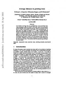
Figure 13. Local synaptic heterogeneities globally increase Functional Network Stability (FuNS). a) Example FuNS traces as a function of normalized synaptic distance from the heterogeneity for networks before (darker colors) and after (lighter colors) introduction of a synaptic heterogeneity. Some values of the simulation parameters result in a distance dependent decrease or no change in FuNS Z-scores (blue traces), while others result in consistent, networkwide significance (red traces). The black, dashed line indicates the normalized distance where FuNS loses significance in the example case shown. Error bars indicate standard error of the mean. b) Normalized distance from the heterogeneity where FuNS significance is lost. Values of one indicate that the global network observes an increase in FuNS due to a localized synaptic heterogeneity. All results averaged over five trials. 2.5 FuNS sensitivity to structural heterogeneity in mixed excitatory and inhibitory networks.

A

CC

Finally, we measure changes in FuNS in response to introduction of network heterogeneity in mixed inhibitory and excitatory networks. Specifically, FuNS is measured as a function of the ratio of total excitation and inhibition generated by neurons in the network (i.e. E/I ratio; Methods 2.1). Generally, we observe that for low values of E/I ratio the reported FuNS is low regardless of the presence of a heterogeneity and, at the same time, a high E/I ratio saturates FuNS in both cases (Figure 14). The greatest response of the networks, in terms of stabilizing dynamics in presence of heterogeneity, is near a balance between excitation and inhibition, i.e. E/I ~ 1 (Figure 14b). Thus, only near such an E/I balance can the dynamics of the network respond in a distributed manner to the introduction of heterogeneity. This provides another piece of evidence that mixed networks near E/I balance increase their dynamic range in response to even localized structural network changes, in agreement with previous studies (Poil et al., 2012; Gautam et al., 2015).

21

SC RI PT

M

A

N

U

Figure 14. Introduction of synaptic heterogeneities maximize increased Functional Network Stability near a balance between excitation and inhibition. a) FuNS as a function of the ratio between excitation and inhibition. Introduction of synaptic heterogeneities (red traces) increases stability over networks missing a synaptic heterogeneity (black traces). b) Difference in FuNS between networks containing and not-containing synaptic heterogeneities. All error bars indicate the standard deviation of the mean, taken over five trials.

A

CC

EP

TE

D

We further compare FCM and FuNS measurements between the fast AMD approach and the CC approach (Figure 15) at the point where FuNS observes a maximum increase in Figure 14b, i.e. E/I ~ 1. As expected, the FCM analysis for both methods is very similar and, indeed, does not show a significant difference between networks with and without a synaptic heterogeneity (Figures 15a and 15b). However, we observe a significant increase in FuNS for the fast AMD method (Figure 15d) but not for the CC method (Figure 15c), assuming a non-normalized Gaussian distribution for both. Thus, though the resulting FCMs are similar, FuNS more accurately picks up on discrete changes in functional network topologies generated using AMD compared to crosscorrelation.

22

SC RI PT U N A M

CC

EP

TE

D

Figure 15. Comparing FC and FuNS between AMD and CC near the E/I Balance. The probability of observing a mean FC value was measured for functional structures from both CC (a) and AMD (b) derived methods, only over the excitatory neurons in the mixed networks, before (black) and after (red) adding a network heterogeneity. The distributions were not significantly different, within a 5% confidence interval (K-S test; CC: p = 0.83, AMD: p=0.54). Similarly, non-normalized Gaussian distributions of FuNS were constructed for CC (c) and AMD (d) before (black) and after (red) introduction of a synaptic heterogeneity. Calculating FuNS for AMD yielded significantly different distributions whereas FuNS for CC did not, within a 5% confidence interval (K-S test; CC: p = 0.09, AMD: p = 𝟕 × 𝟏𝟎−𝟗). Error bars represent standard error of the mean, whereas Gaussian widths stem from the standard deviation. Averaged over 5 trials.

3. FuNS applied to in vivo data

A

Finally, we wanted to know whether functional connectivity and stability changes could be detected following network reorganization in vivo (Figure 16). We hypothesize that synaptic plasticity in hippocampal area CA1 following single-trial contextual fear conditioning (CFC) (Tronson et al., 2009) is a plausible biological model to investigate how rapid structural network changes underlying memory formation affects network dynamics. CA1 network activity is necessary for fear memory consolidation in the hours following CFC (Daumas et al., 2005). For this reason, we recorded the same population of CA1 neurons from C57BL/6J mice over a 24-h baseline and for 24 h following CFC (placement into a novel environmental context, followed 2.5 23

CC

EP

TE

D

M

A

N

U

SC RI PT

min later by a 0.75 mA foot shock) to determine how functional network dynamics are affected by de novo memory formation. CFC affects many aspects of CA1 network dynamics; for a detailed description of the obtained results, please refer to (Ognjanovski et al., 2014, 2017). The results presented here focus on comparing performance of the metrics (fast AMD and CC, both together with FuNS assessment) for the case when mouse was subjected to successful

A

Figure 16. Application of AMD and FSM to in vivo mouse data. We extracted spike data from intervals of slow wave sleep across 6-hour recordings for both before (baseline) and after (post stimulation) the contextual fear conditioning. The spike trains were first divided into multiple one-minute bins, then the functional connectivity (FC) pattern for each bin is calculated by bidirectional AMD and CC. We compared the distribution of both FC values (a,b) and stability values (c,d). For FC values, the elements are extracted collectively from all the FCMs. The histogram shows us that AMD is able to capture the functional connectivity changes from baseline to post contextual fear conditioning more sensitively than CC. For stability values, the elements were extracted from the FSMs for baseline and post-stimulation respectively, and calculated as described in Results 1.4. We observe significant shift in stability for both CC and AMD calculation, however, AMD gives a more statistically significant separation between the two distributions. 24

SC RI PT

memory consolidation (success was determined by observing behavioral changes 24 hours after training). First, the 6-hour baseline and 6-hour post stimulation are divided into 1-minute time windows, and FCMs are calculated in each bin, which are further used to calculate FSM. Figure 16 shows comparisons of the distribution of functional connectivity values (Figures 16a and 16b) and stability values (Figures 16c and 16d). Comparing with CC, AMD is shown to be more sensitive to capture the change of functional connectivity and stability in the network during memory consolidation. Furthermore, the more significant shift of similarity distribution indicates that stability is a better measurement of the change in global network properties.

Discussion

A

CC

EP

TE

D

M

A

N

U

The advent of new recording techniques allowing for prolonged recordings from an increasing number of neurons in the brain drives the necessity to develop new analysis tools to meaningfully process data. Two underlying issues however need to be overcome. First, there is a severe under-sampling problem: how is it possible to identify universal properties of neuronal dynamics during information processing if the number of recorded cells remain tremendously small in comparison with number of cells participating in the computation? Second, and related to the first question, is how to characterize the data so that the (small) recorded population provides a representative picture of the dynamics of whole modality? Solutions to the latter attempt to bridge the timescales between neuronal activity and behavioral states which they encode, while prolonged recordings on freely behaving mice are now possible, they generate enormous data sets which need to be meaningfully processed in a finite amount of time. In this paper we have addressed both of these problems - we have introduced a framework, based on the AMD between spikes in individual neurons’ recorded spike trains, which allows for rapid assessment of network functional connectivity structure throughout extended time periods. We showed that we can extend the developed metrics so that we can rapidly estimate significance of functional connectivity between neuronal pairs, based on analysis of distribution of ISI intervals of the neurons in question, not only without loss of resolution, but often with improved sensitivity as compared to cross-correlation based methods. At the same time, rapid assessment of significance allows us to speed up functional connectivity reconstruction by a couple of orders of magnitude, primarily due to the fact that we can bypass typical bootstrapping methods without loss of accuracy (Results 1.1-1.5). Further, we used this fast, AMD-based method to reconstruct instantaneous functional connectivity within the network and subsequently introduced Functional Network Stability (FuNS), a measure that assesses the temporal stability of functional connectivity networks. We showed that FuNS is especially useful in detecting changes in network-wide dynamics due to discrete changes in network structural connectivity, referred to here as synaptic heterogeneities. Namely, we show that localized and relatively small heterogeneities can induce dynamical changes throughout the entire network, as is evidenced by high FuNS in neuronal groups distantly connected to the heterogeneity region (Figure 14). This in turn allows for robust detection of such changes experimentally, even in the conditions of severe under-sampling (Skilling et al., 2017; Ognjanovski et al., 2017). These results indicate that while reconstruction of functional connectivity between the recorded neurons may yield ambiguous results as the functional relation of the recorded cells to the computational task is unknown, the changes in the global dynamics of the representations is a more robust measure of local network changes in response to computational tasks. (Results 2.1-2.4) To better exemplify this point, we used both model simulations and in vivo 25

TE

D

M

A

N

U

SC RI PT

experimental recordings to show that discrete changes to network structure may yield ambiguous results in terms of reconstruction of detailed changes in functional network connectivity, but at the same time show robust stabilization of dynamical network representations (Results 3.1). Finally, we investigate whether observed stabilization of dynamical network representations can inform us about universal network properties that are underlying the computation. Here, we show that in mixed excitatory-inhibitory networks, the highest sensitivity (in terms of changes in global network representations) to introduction of localized heterogeneity is achieved near a balance between excitation and inhibition (E/I balance; Results 2.5). This result is in line with other existing results which have shown that E/I balance emerges naturally in neural networks (Vreeswijik and Sompolinsky, 1996) and that neurons operating in networks near E/I balance exhibit faster linear responses to stimulation, and greater dynamic range (Vreeswijik and Sompolinsky, 1996). Recent findings have also shown that E/I balance is required for heightened neuronal selectivity (Rubin et al., 2017). Altogether, we believe that the introduced framework for rapid calculation of functional network connectivity allows for robust analysis of multiunit recordings. Numerous linear and nonlinear, methods have been developed over the last decade to reconstruct and characterize functional network connectivity. We have earlier compared the performance of functional grouping based on AMD assessment to some of these methods (Feldt et al., 2009). Many of the developed tools require assessment of functional adjacency matrix. We believe that the algorithm proposed here provides a robust alternative for the commonly used cross-correlation method. Further we believe that fast AMD together with evaluation of FuNS helps to overcome two major constraints in neuroscience: undersampling and the difficulty of bridging diverse timescales of neuronal dynamics and cognition. We believe that this framework will be widely applicable to numerous problems in systems neuroscience. Conflicts of Interest: The authors declare no competing financial interests.

EP

Acknowledgements

The work was supported by NIH NIBIB grant no. 5 R01 EB018297.

CC

References

A

Barral J, Reyes AD (2016) Synaptic scaling rule preserves excitatory–inhibitory balance and salient neuronal network dynamics. Nat Neurosci 19(12):1690-1696. Bassett DS, Greenfield DL, Meyer-Lindenberg A, Weinberger DR, Moore SW, Bullmore ET (2010) Efficient physical embedding of topologically complex information processing networks in brains and computer circuits. PLoS Comput. Biol. 6, e1000748.

26

Bassett DS, Wymbs NF, Porter MA, Mucha PJ, Carlson JM, Grafton ST (2011) Dynamic reconfiguration of human brain networks during learning. Proc Natl Acad Sci U S A. 108(18):7641-6. Bastos AM, Schoffelen JM (2016) A Tutorial Review of Functional Connectivity Analysis Methods and Their Interpretational Pitfalls. Front. Syst. Neurosci. 9:175.

SC RI PT

Berg RW, Alaburda A, Hounsgaard J (2007) Balanced Inhibition and Excitation Drive Spike Activity in Spinal Half-Centers. Science 315(5810): 390-393. Boccaletti S, Latora V, Moreno Y, Chavez M, Hwang DU. (2006) Complex networks: structure and dynamics. Phys. Rep. 424: 175–308. Buzsaki, G. (2004) Large-scale recording of neuronal ensembles. Nat. Neurosci. 7: 446–451.

Cestnik R, Rosenblum M (2017) Reconstructing networks of pulse-coupled oscillators from spike trains. arXiv nlin arXiv:1704.06224v1.

N

U

Chorev E, Epsztein J, Houweling AR, Lee AK, Brecht M (2009) Electrophysiological recordings from behaving animals–going beyond spikes. Curr. Opin. Neurobiol. 19: 513–519.

A

Cimenser A, Purdon PL, Pierce ET, Walsh JL, Salazar-Gomez AF, Harrell PG, Tavares-Stoeckel C, Habeeb K, Brown EN (2011) Tracking brain states under general anesthesia by using global coherence analysis. Proc Natl Acad Sci U S A 108(21): 8832-7.

D

M

Daumas S, Halley H, Francés B, and Lassalle J.M (2005) Encoding, consolidation, and retrieval of contextual memory: differential involvement of dorsal CA3 and CA1 hippocampal subregions. Learn Mem 12(4): 375–82.

TE

Davison EN, Schlesinger KJ, Bassett DS, Lynall ME, Miller MB, Grafton ST, and Carlson JM (2015) Brain Network Adaptability across Task States. PLoS Comput Biol 11(1): e1004029.

EP

De Vico Fallani F, Richiardi J, Chavez M, Achard S (2014) Graph analysis of functional brain networks: practical issues in translational neuroscience. Philos Trans R Soc Lond B Biol Sci. 369(1653). Feldman DE (2012) The spike-timing dependence of plasticity. Neuron 75(4):556-71.

CC

Feldt S, Waddell J, Hetrick VL, Berke JD, Zochowski M (2009) Functional clustering algorithm for the analysis of dynamic network data. Phys Rev E Stat Nonlin Soft Matter Phys 79: 056104.

A

Feldt S, Bonifazi P, Cossart R (2011) Dissecting functional connectivity of neuronal microcircuits: experimental and theoretical insights? Trends Neurosci. 34(5):225-36. Friston K, Moran R, Seth AK (2013) Analysing connectivity with Granger causality and dynamic causal modelling. Current Opinion in Neurobiology 23(2): 172–178. Froemke RC (2015) Plasticity of Cortical Excitatory-Inhibitory Balance. Annual Review of Neuroscience 38:195-219.

27

Gautam SH, Hoang TT, McClanahan K, Grady SK, Shew WL (2015) Maximizing sensory dynamic range by tuning the cortical state to criticality. PLoS Comput Biol 11(12): e1004576. Ghiani CA, Beltran-Parrazal L, Sforza DM, Malvar JS, Seksenyan A, Cole R, Smith DJ, Charles A, Ferchmin PA, de Vellis J (2007) Genetic program of neuronal differentiation and growth induced by specific activation of NMDA receptors. Neurochem Res 32(2): 363-76.

SC RI PT

Gu S, Pasqualetti F, Cieslak M, Telesford QK, Yu AB, Kahn AE, Medaglia JD, Vettel JM, Miller MB, Grafton ST, Bassett DS (2015) Controllability of structural brain networks. Nat Commun 6:8414. Hermundstad AM, Brown KS, Bassett DS, and Carlson JM (2011) Learning, Memory, and the Role of Neural Network Architecture. PLoS Comput Biol 7(6): e1002063. Lichtman JW, Livet J, Sanes JR (2008) A technicolour approach to the connectome. Nat. Rev. Neurosci. 9: 417–422.

U

Luo L, Callaway EM, Svoboda K (2008) Genetic dissection of neural circuits. Neuron 57: 634– 660.

A

N

Medaglia JD, Pasqualetti F, Hamilton RH, Thompson-Schill SL, Bassett DS (2017) Brain and cognitive reserve: Translation via network control theory. Neurosci Biobehav Rev 75:53-64.

M

Misic B, Sporns O (2016) From regions to connections and networks: new bridges between brain and behavior. Current Opinion in Neurobiology 40:1-7.

D

Nakhnikian A, Rebec GV, Grasse LM, Dwiel LL, Shimono M, Beggs JM (2014) Behavior modulates effective connectivity between cortex and striatum. PLoS One 9(3):e89443.

TE

Newman, ME (2004) Fast algorithm for detecting community structure in networks. Phys. Rev. E: Stat. Nonlin. Soft Matter Phys. 69, 066133.

EP

Newman, ME (2006) Finding community structure in networks using the eigenvectors of matrices. Phys. Rev. E: Stat. Nonlin. Soft Matter Phys. 74, 036104. Newman, ME (2010) Networks: An Introduction. Oxford University Press.

CC

Nigam S, Shimono M, Ito S, Yeh FC, Timme N, Myroshnychenko M, Lapish CC, Tosi Z, Hottowy P, Smith WC, Masmanidis SC, Litke AM, Sporns O, Beggs JM (2016) Rich-Club Organization in Effective Connectivity among Cortical Neurons. J Neurosci 36(3):670-84.

A

Ognjanovski N, Maruyama D, Lashner N, Zochowski M, Aton SJ (2014) CA1 hippocampal network activity changes during sleep-dependent memory consolidation. Front Syst Neurosci. 8:61. Ognjanovski N, Schaeffer S, Wu J, Mofakham S, Maruyama D, Zochowski M, Aton SJ (2017) Parvalbumin-expressing interneurons coordinate hippocampal network dynamics required for memory consolidation. Nat Commun 8:15039.

28

Pajevic S, Plenz D (2009) Efficient network reconstruction from dynamical cascades identifies small-world topology of neuronal avalanches. PLoS Comput Biol 5(1):e1000271. Park HJ, Friston K (2013) Structural and Functional Brain Networks: From Connections to Cognition. Science 342, Issue 6158.

SC RI PT

Petersen SE, Sporns O (2015) Brain Networks and Cognitive Architectures. Neuron 88(1): 207219. Poil SS, Hardstone R, Mansvelder HD, Linkenkaer-Hansen K (2012) Critical-State Dynamics of Avalanches and Oscillations Jointly Emerge from Balanced Excitation/Inhibition in Neuronal Networks. Journal of Neuroscience 32(29):9817-23. Poli D, Pastore VP, Martinoia S, Massobrio P (2016) From functional to structural connectivity using partial correlation in neuronal assemblies. J. Neural Eng. 13(2):026023.

U

Ponten SC, Daffertshofer A, Hillebrand A, Stam CJ (2010) The relationship between structural and functional connectivity: Graph theoretical analysis of an EEG neural mass model. NeuroImage 52: 985-994.

A

N

Rubin R, Abbott LF, Sompolinsky H (2017) Balanced Excitation and Inhibition are required for High-Capacity, Noise-Robust Neuronal Selectivity. arXiv q-bio arXiv:1705.01502.

M

Rubinov M, Sporns O (2010) Complex network measures of brain connectivity: Uses and interpretations. NeuroImage 52: 1059-1069.

D

Shen K, Hutchison RM, Bezgin G, Everling S, McIntosh AR (2015) Network Structure Shapes Spontaneous Functional Connectivity Dynamics. Journal of Neuroscience 35(14):5579-88.

TE

Shimono M, Beggs JM (2015) Functional Clusters, Hubs, and Communities in the Cortical Microconnectome. Cereb Cortex 25(10):3743-57.

EP

Skilling QM, Maruyama D, Ognjanovski N, Aton S, Zochowski M (2017) Criticality, stability, competition, and consolidation of new representations in brain networks. arXiv 1702.07649.

CC

Song S, Miller KD, Abbott LF (2000) Competitive Hebbian learning through spike-timingdependent synaptic plasticity. Nature Neurosci 3: 919-926.

A

Sporns O, Tononi G, Edelman GM (2000) Theoretical Neuroanatomy: Relating Anatomical and Functional Connectivity in Graphs and Cortical Connection Matrices. Cerebral Cortex 10(2): 127– 141. Stafford JM, Jarrett BR, Miranda-Dominguez O, Mills BD, Cain N, Mihalas S, Lahvis GP, Lattal KM, Mitchell SH, David SV, Fryer JD, Nigg JT, Fair DA (2014) Large-scale topology and the default mode network in the mouse connectome. Proc. Natl. Acad. Sci. U S A. 111(52):18745-50. Supekar K, Menon V, Rubin D, Musen M, Greicius M (2008) Network Analysis of Intrinsic Functional Brain Connectivity in Alzheimer's Disease. PlOS Comp Biology 4(6): e1000100.

29

Tronson NC, Schrick C, Huh KH, Srivastava DP, Penzes P, Guedea AL, Gao C, Radulovic J (2009) Segregated Populations of Hippocampal Principal CA1 Neurons Mediating Conditioning and Extinction of Contextual Fear. J Neurosci 29(11): 3387-94. Vanderhaeghen P, Cheng HJ (2010) Guidance molecules in axon pruning and cell death. Cold Spring Harb Perspect Biol 2(6): a001859.

SC RI PT

Vreeswijik C, Sompolinsky H (1996) Chaos in neuronal network with balanced excitatory and inhibitory activity. Science 274(5293): 1724-6. Wang HE, Bénar CG, Quilichini PP, Friston KJ, Jirsa VK, Bernard C (2014) A systematic framework for functional connectivity measures. Front Neurosci. 8: 405.

A

CC

EP

TE

D

M

A

N

U

Zaytsev YV, Morrison A, Deger M (2015) Reconstruction of recurrent synaptic connectivity of thousands of neurons from simulated spiking activity. J Comput Neurosci 39:77–103.

30