Functional Renormalization Group and the Field Theory of Disordered ...

Functional Renormalization Group and the Field Theory of Disordered Elastic Systems ¨ Pierre Le Doussal1 , Kay Jorg Wiese2 and Pascal Chauve3 1

2

CNRS-Laboratoire de Physique Th´eorique de l’Ecole Normale Sup´erieure, 24 rue Lhomond, 75005 Paris, France Kavli Institute of Theoretical Physics, University of California at Santa Barbara, Santa Barbara, CA 93106-4030, USA 3 CNRS-Laboratoire de Physique des Solides, Universit´e de Paris-Sud, Bˆat. 510, 91405 Orsay, France

arXiv:cond-mat/0304614v1 27 Apr 2003

(Dated: April 26, 2003) We study elastic systems such as interfaces or lattices, pinned by quenched disorder. To escape triviality as a result of “dimensional reduction”, we use the functional renormalization group. Difficulties arise in the calculation of the renormalization group functions beyond 1-loop order. Even worse, observables such as the 2-point correlation function exhibit the same problem already at 1-loop order. These difficulties are due to the non-analyticity of the renormalized disorder correlator at zero temperature, which is inherent to the physics beyond the Larkin length, characterized by many metastable states. As a result, 2-loop diagrams, which involve derivatives of the disorder correlator at the non-analytic point, are naively “ambiguous”. We examine several routes out of this dilemma, which lead to a unique renormalizable field-theory at 2-loop order. It is also the only theory consistent with the potentiality of the problem. The β-function differs from previous work and the one at depinning by novel “anomalous terms”. For interfaces and random bond disorder we find a roughness exponent ζ = 0.20829804ǫ + 0.006858ǫ2 , ǫ = 4 − d. For random field disorder we find ζ = ǫ/3 and compute universal amplitudes to order O(ǫ2 ). For periodic systems we evaluate the universal amplitude of the 2-point function. We also clarify the dependence of universal amplitudes on the boundary conditions at large scale. All predictions are in good agreement with numerical and exact results, and an improvement over one loop. Finally we calculate higher correlation functions, which turn out to be equivalent to those at depinning to leading order in ǫ.

I. INTRODUCTION Elastic objects pinned by quenched disorder are central to the physics of disordered systems. In the last decades a considerable amount of research has been devoted to them. From the theory side they are among the simplest, but still quite non-trivial, models of glasses with complex energy landscape and many metastable states. They are related to a remarkably broad set of problems, from subsequences of random permutations in mathematics [1, 2, 3], random matrices [4, 5] to growth models [6, 7, 8, 9, 10, 11, 12, 13, 14] and Burgers turbulence in physics [15, 16], as well as directed polymers [6, 17] and optimization problems such as sequence alignment in biology [18, 19, 20]. Foremost, they are very useful models for numerous experimental systems, each with its specific features in a variety of situations. Interfaces in magnets [21, 22] experience either short-range disorder (random bond RB), or long range (random field RF). Charge density waves (CDW) [23] or the Bragg glass in superconductors [24, 25, 26, 27, 28] are periodic objects pinned by disorder. The contact line of liquid helium meniscus on a rough substrate is governed by long range elasticity [29, 30, 31]. All these systems can be parameterized by a N -component height or displacement field ux , where x denotes the d-dimensional internal coordinate of the elastic object (we will use uq to denote Fourier components). An interface in the 3D random field Ising model has d = 2, N = 1, a vortex lattice d = 3, N = 2, a contact-line d = 1 and N = 1. The so-called directed polymer (d = 1) has been much studied [32] as it maps onto the Kardar-Parisi-Zhang growth model [6] for any N . The equilibrium problem is defined by the partition function

Z=

R

D[u] exp(−H[u]/T ) associated to the Hamiltonian Z 1 H[u] = dd x (∇u)2 + V (ux , x) , (1.1) 2

which is the sum of an elastic energy which tends to suppress fluctuations away from the perfectly ordered state u = 0, and a random potential which enhances them. The resulting roughness exponent ζ h(u(x) − u(x′ ))2 i ∼ |x − x′ |2ζ

(1.2)

is measured in experiments for systems at equilibrium (ζeq ) or driven by a force f . Here and below h. . . i denote thermal averages and (. . . ) disorder ones. In some cases, long-range elasticity appears e.g. for the contact line by integrating out the bulk-degrees of freedom [31], corresponding to q 2 → |q| in the elastic energy. As will become clear later, the random potential can without loss of generality be chosen Gaussian with second cumulant V (u, x)V (u′ , x′ ) = R(u − u′ )δ d (x − x′ ) .

(1.3)

with various forms: Periodic systems are described by a periodic function R(u), random bond disorder by a short-range function and random field disorder of variance σ by R(u) ∼ −σ|u| at large u. Although this paper is devoted to equilibrium statics, some comparison with dynamics will be made and it is thus useful to indicate the equation of motion η∂t uxt = c∇2x uxt + F (x, uxt ) + f ,

(1.4)

with friction η. The pinning force is F (u, x) = −∂u V (u, x) of correlator ∆(u) = −R′′ (u) in the bare model.

2 Despite some significant progress, the model (1.1) has mostly resisted analytical treatment, and one often has to rely on numerics. Apart from the case of the directed polymer in 1+1 dimensions (d = 1, N = 1), where a set of exact and rigorous results was obtained [2, 5, 33, 34, 35], analytical methods are scarce. Two main analytical methods exist at present, both interesting but also with severe limitations. The first one is the replica Gaussian Variational Method (GVM) [36]. It is a mean field method, which can be justified for N = ∞ and relies on spontaneous replica symmetry breaking (RSB) [37, 38]. Although useful as an approximation, its validity at finite N remains unclear. Indeed, it seems now generally accepted that RSB does not occur for low d and N . The remaining so-called weak RSB in excitations [39, 40, 41] may not be different from a more conventional droplet picture. Another exactly solvable mean field limit is the directed polymer on the Cayley tree, which also mimics N → ∞ and there too it is not fully clear how to meaningfully expand around that limit [42, 43, 44]. The second main analytical method is the Functional Renormalization Group (FRG) which attempts a dimensional expansion around d = 4 [26, 28, 45, 46, 47]. The hope there is to include fluctuations, neglected in the mean field approaches. However, until now this method has only been developed to one loop, for good reasons, as we discuss below. Its consistency has never been checked or tested in any calculation beyond one loop (i.e. lowest order in ǫ = 4 − d). Thus contrarily to pure interacting elastic systems (such as e.g. polymers) there is at present no quantitative method, such as a renormalizable field theory, which would allow to compute accurately all universal observables in these systems. The central reason for these difficulties is the existence of many metastable states (i.e. local extrema) in these systems. Although qualitative arguments show that they arise beyond the Larkin length [48], these are hard to capture by conventional field theory methods. The best illustration of that is the so called dimensional reduction (DR) phenomenon, which renders naive perturbation theory useless [21, 49, 50, 51, 52, 53] in pinned elastic systems as well as in a wider class of disordered models (e.g. random field spin models). Indeed it is shown that to any order in the disorder at zero temperature T = 0, any physical observable is found to be identical to its (trivial) average in a Gaussian random force (Larkin) model, e.g. ζ = (4 − d)/2 for RB disorder. Thus perturbation theory appears (naively) unable to help in situations where there are many metastable states. The two above mentioned methods (GVM and FRG) are presently the only known ways to escape dimensional reduction and to obtain non-trivial values for ζ (in two different limits but consistent when they can be compared [26, 28, 47]). The mean field method accounts for metastable states by RSB. This however may go further than needed since it implies a large number of pure states (i.e. low (free) energy states differing by O(T ) in (free) energy). The other method, the FRG, captures metastability through a non-analytic action with a cusp singularity. Both the RSB and the cusp arise dynamically, i.e. spontaneously, in the limits studied. The 1-loop FRG has had some success in describing pinned systems. It was noted by Fisher [46] within a Wilson scheme

analysis of the interface problem in d = 4 − ǫ that the coarse grained disorder correlator becomes non-analytic beyond the Larkin scale Lc , yielding large scale results distinct from naive perturbation theory. Within this approach an infinite set of operators becomes relevant in d < 4, parameterized by the second cumulant R(u) of the random potential. Explicit solution of the 1-loop FRG for R(u) gives several non-trivial attractive fixed points (FP) to O(ǫ) proposed in [46] to describe RB, RF disorder and in [26, 28], periodic systems such as CDW or vortex lattices. All these fixed points exhibit a “cusp” singularity as R∗′′ (u) − R∗′′ (0) ∼ |u| at small |u|. The cusp was interpreted in terms of shocks in the renormalized force [54], familiar from the study of Burgers turbulence (for d = 1, N = 1). The dynamical FRG was also developed to one loop [55, 56, 57] to describe the depinning transition. The mere existence of a non-zero critical threshold force fc ∼ |∆′ (0+ )| > 0 is a direct consequence of the cusp (it vanishes for an analytic force correlator ∆(u)). Extension to non-zero temperature T > 0 suggested that the cusp is rounded within a thermal boundary layer u ∼ T L−θ . This was interpreted to describe thermal activation and leads to a reasonable derivation of the celebrated creep law for activated motion [58, 59]. In standard critical phenomena a successful 1-loop calculation usually quickly opens the way for higher loop computations, allowing for accurate calculation of universal observables and comparison with simulations and experiments, and eventually a proof of renormalizability. In the present context however, no such work has appeared in the last fifteen years since the initial proposal of [46], a striking sign of the high difficulties which remain. Only recently a 2-loop calculation was performed [60, 61] but since this study is confined to an analytic R(u) it only applies below the Larkin length and does not consistently address the true large scale critical behavior. In fact doubts were even raised [47] about the validity of the ǫ-expansion beyond order ǫ. It is thus crucial to construct a renormalizable field theory, which describes statics and depinning of disordered elastic systems, and which allows for a systematic expansion in ǫ = 4 − d. As long as this is not achieved, the physical meaning and validity of the 1-loop approximation does not stand on solid ground and thus, legitimately, may itself be called into question. Indeed, despite its successes, the 1-loop approach has obvious weaknesses. One example is that the FRG flow equation for the equilibrium statics and for depinning are identical, while it is clear that these are two vastly different physical phenomena, depinning being irreversible. Also, the detailed mechanism by which the system escapes dimensional reduction in both cases is not really elucidated. Finally, there exists no convincing scheme to compute correlations, and in fact no calculation of higher than 2-point correlations has been performed. Another motivation to investigate the FRG is that it should apply to other disordered systems, such as random field spin models, where dimensional reduction also occurs and progress has been slow [45, 62, 63, 64, 65]. Insight into model (1.1) will thus certainly lead to progresses in a broader class of disordered systems.

3 In this paper we construct a renormalizable field theory for the statics of disordered elastic systems beyond one loop. The main difficulty is the non-analytic nature of the theory (i.e. of the fixed point effective action) at T = 0. This makes it a priori quite different from conventional field theories for pure systems. We find that the 2-loop diagrams are naively “ambiguous”, i.e. it is not obvious how to assign a value to them. We want to emphasize that this difficulty already exists at one loop, e.g. even the simplest one loop correction to the two point function is naively “ambiguous”. Thus it is not a mere curiosity but a fundamental problem with the theory, “swept under the rug” in all previous studies, but which becomes unavoidable to confront at 2-loop order. It originates from the metastability inherent in the problem. For the related theory of the depinning transition, we have shown in companion papers [66, 67] how to surmount this problem and we constructed a 2-loop renormalizable field theory from first principles. There, all ambiguities are naturally lifted using the known exact property that the manifold only moves forward in the slowly moving steady state. Unfortunately in the statics there is no such helpful property and the ambiguity problem is even more arduous. Here we examine the possible ways of curing these difficulties. We find that the natural physical requirements, i.e. that the theory should be (i) renormalizable (i.e. that a universal continuum limit exists independent of short-scale details), (ii) that the renormalized force should remain potential, and (iii) that no stronger singularity than the cusp in R′′ (u) should appear to two loop (i.e. no “supercusp”), are rather restrictive and constrain possible choices. We then propose a theory which satisfies all these physical requirements and is consistent to two loops. The resulting β-function differs from the one derived in previous studies [60, 61] by novel static “anomalous terms”. These are different from the dynamical “anomalous terms” obtained in [66, 67, 68] showing that indeed depinning and statics differ at two loop, fulfilling another physical requirement. We then study the fixed points describing several universality classes, i.e. the interface with RB and RF disorder, the random periodic problem, and the case of LR elasticity. We obtain the O(ǫ2 ) corrections to several universal quantities. The prediction for the roughness exponent ζ for random bond disorder has the correct sign and order of magnitude to notably improve the precision as compared to numerics in d = 3, 2 and to match the exact result ζ = 2/3 in d = 1. For random field disorder we find ζ = ǫ/3 which, for equilibrium is likely to hold to all orders. By contrast, non-trivial corrections of order O(ǫ2 ) were found for depinning [66, 67]. The amplitude, which in that case is a universal function of the random field strength is computed and it is found that the 2loop result also improves the agreement as compared to the exact result known [69] for d = 0. For the periodic CDW case we compare with the numerical simulations in d = 3 and obtain reasonable agreement. Some of the results of this paper were briefly described in a short version [66] and agree with a companion study using exact RG [70, 71]). Since the physical results also seem to favor this theory we then look for better methods to justify the various assumptions. We found several methods which allow to lift ambigu-

ities and all yield consistent answers. A detailed discussion of these methods is given. In particular we find that correlation functions can be unambiguously defined in the limit of a small background field which splits apart quasi-degenerate states when they occur. This is very similar to what was found in a related study where we obtained the exact solution of the FRG in the large N limit [72]. Finally, the methods introduced here will be used and developed further to obtain a renormalizable theory to three loops, and compute its β-function in [73]. Let us mention that a first principles method which avoids ambiguities is to study the system at T > 0. However, this turns out to be highly involved. It is attempted via exact RG in [70] and studied more recently in [74, 75] where a field theory of thermal droplet excitation was constructed. A short account of our work has appeared in [66], and a short pedagogical introduction is given in [76]. The outline of this paper is as follows. In Section II we explain in a detailed and pedagogical way the perturbation theory and the power counting. In Section III we compute the 1-loop (Section III A) and 2-loop (Section III B) corrections to the disorder. The calculation of the repeated 1-loop counter-term is given in Section III C. In Section III D we identify the values for ambiguous graphs. This yields a renormalizable theory with a finite β-function, which is potential and free of a supercusp. The more systematic discussion of these ambiguities is postponed to Section V. We derive the βfunction and in Section IV present physical results, exponents and universal amplitudes to O(ǫ2 ). Some of these quantities are new, and have not yet been tested numerically. In Section V we enumerate all the methods which aim at lifting ambiguities and explain in details several of them which gave consistent results. In Section VI we detail the proper definition and calculation of correlation functions. In Appendix A and B we present two methods which seem promising but do not work, in order to illustrate the difficulties of the problem. In Appendix F we present a summary of all one and 2-loop corrections including finite temperature. In Appendix D we give details of calculations for what we call the sloop elimination method. The reader interested in the results can skip Section II and Section III and go directly to Section IV. The reader interested in the detailed discussion of the problems arising in this field theory should read Section V.

II. MODEL AND PERTURBATION THEORY A. Replicated action and effective action We study the static equilibrium problem using replicas, i.e. consider the partition sum in presence of sources:

Z[j] =

Z Y a

D[ua ] exp −S[u] +

Z X x

a

jxa uax

!

, (2.1)

4 from which all static observables can be obtained. The action S and replicated Hamiltonian corresponding to (1.1) are Z X 1 H[u] = [(∇uax )2 + m2 uax ] S[u] = T 2T x a Z X 1 − 2 R(uax − ubx ) . (2.2) 2T x ab

a runs from 1 to n and the limit of zero number of replicas n = 0 is implicit everywhere. We have added a small mass which confines the interface inside a quadratic well, and provides an infrared cutoff. We are interested in the large scale limit m → 0. We will denote Z Z dd q := (2.3) (2π)d q Z Z := dd x . (2.4) x

For periodic systems the integration is over the first Brillouin zone. A short-scale UV cutoff is implied at q ∼ Λ, but for actual calculations we find it more convenient to use dimensional regularization. We also consider the effective action functional Γ[u] associated to S. It is, as we recall [77, 78], the Legendre transform of the generating function of connected correlations W[j] = ln Z[j], thus defined by eliminating j in Γ[u] = ju − W[j], W ′ [j] = u. If we had chosen non-Gaussian disorder additional terms with free sums over p replicas (called p-replica terms) corresponding to higher cumulants of disorder would be present in (2.2), together with a factor of 1/T p. These terms are generated in the perturbation expansion, i.e. they are present in Γ[u]. We do not include them in (2.2) because, as we will see below, these higher disorder cumulants are not relevant within (conventional) power counting, so for now we ignore them. The temperature T appears explicitly in the replicated action (2.2), although we will focus on the T = 0 limit. Because the disorder distribution is translation invariant, the disorder term in the above action is invariant under the so called statistical tilt symmetry [17, 79] (STS), i.e. the shift uax → uax + gx . One implication of STS is that the 1-replica replica part of the action (i.e. the first line of 2.2) is uncorrected by disorder, i.e. it is the same in Γ[u] and S[u] [80]. Since the elastic coefficient is not renormalized, we have set it to unity. B. Diagrammatics, definitions We first study perturbation theory, its graphical representation and power counting. Everywhere in the paper we denote the exact 2-point correlation by Cab (x − y), i.e. in Fourier: huaq ubq′ i = (2π)d δ d (q + q ′ )Cab (q)

(2.5)

while the free correlation function (from the elastic term) used for perturbation theory in the disorder is denoted by Gab (x − y) = δab G(x − y) and reads in Fourier: huaq ubq′ i0 = (2π)d δ d (q + q ′ )Gab (q) T Gab (q) = 2 δab , q + m2

(2.6) (2.7)

FIG. 1: Each diagram with unsplitted vertices contains several diagrams with splitted vertices: here the 1-loop unsplitted diagram (top) generates three possible topologically distinct splitted diagrams, two (shown here, bottom) are 2-replica terms, the third one, i.e. (a) in Fig. (2) is a three replica term

which is represented graphically by a line: a

b

=

T δab . q 2 + m2

(2.8)

Each propagator thus carries one factor of G(q) = T /(q 2 + m2 ). Each disorder interaction vertex comes with a factor of 1/T 2 and gives one momentum conservation rule. Since each disorder vertex is a function, an arbitrary number of lines can come out of it. k lines coming out of a vertex result in k derivatives R(k) after Wick contractions = R(k) .

(2.9)

Since each disorder vertex contains two replicas it is sometimes convenient to use “splitted vertices” rather than “unsplitted ones”. Thus we call “vertex” an unsplitted vertex and we call a “point” the half of a vertex. a b

=

X R(ua − ub ) ab

2T 2

.

(2.10)

Each unsplitted diagram thus gives rise to several splitted diagrams, as illustrated in Fig. 1 One can define the number of connected components in a graph with splitted vertices. Since each propagator identifies two replicas, a p-replica term contains p connected components. When the 2-points of a vertex are connected, this vertex is said to be “saturated”. It gives a derivative evaluated at zero R(k) (0). Standard momentum loops are loops with respect to unsplitted vertices, while we call “sloops” the loops with respect to points (in splitted diagrams). This is illustrated in Fig. (2) The momentum 1-loop and 2-loop diagrams which correct the disorder at T = 0 are shown in Fig. 3 (unsplitted vertices). There are three types of 2-loop graphs A, B and C. Since they have two vertices (a factor R/T 2 each) and three propagators (a factor of T each) the graphs E and F lead to corrections to R proportional to temperature and will not be studied here (see however Appendix F). It is important to distinguish between fully saturated diagrams and functional diagrams. The FS diagrams are those needed for a full average, e.g. a correlation function. There all fields are contracted and one is only left with the space dependence. These are the standard diagrams in more conventional polynomial field theories such as φ4 . Then all vertices are evaluated at u = 0, yielding products of derivatives R(k) (0).

5 tain saturated vertices, whose space and field dependence disappears (such as (c) in Fig. 2) and that the limit n → 0 does not produce constraints. An example is the calculation of Γ[u] since one can always attach additional external legs to any point by taking a derivative with respect to the field u.

(a) (b) (c) FIG. 2: Graphs (a) (a 1-loop diagram) and (b) (a 2-loop diagram) each contains three connected components. Since each contain one “sloop” they are both three replica terms proportional to T . The left vertex on diagram (c) is “saturated” : replica indices are constrained to be equal and thus the diagram does not depend on the left space point.

C A

E G

B

D

F

FIG. 3: unsplitted diagrams to one loop D, one loop with inserted 1-loop counter-term G and 2-loop diagrams A, B, C, E and F.

These are also the graphs which come in the standard expansion of Γ[u] in powers of u which generate the “proper” or “renormalized” vertices, i.e. the sum over all 1-particle irreducible graphs with some external legs, from which all correlations can be obtained. Note that in the fully saturated diagrams there can be no free point, all points in a vertex have to be connected to some propagator (and to some external replica) otherwise there is a free replica sum yielding a factor of n and a vanishing contribution in the limit of n = 0. However, since we have to deal with a function R(u) we will more often consider functional diagrams. A functional diagram still depends on the field u. It can depend on u at several points in space (multi-local term), as for example:

x

y

∼

X R′ (ua − ub ) R′ (uay − ucy ) x

abc

2T 2

x

2T 2

T G(x−y)

(2.11) Such a graph with p connected components corresponds to a p replica functional term. Or it can represent the projection of such a term onto a local part, as arises in the standard operator product expansion (OPE): X R′ (ua − ub ) R′ (ua − uc ) Z x x x x ∼ G(x−y) . T 2T 2 2T 2 y abc (2.12) Typically using functional diagrams we want to compute the effective action functional Γ[u], or its local part, i.e. its value for a spatially uniform mode uax = ua , which includes the corrections to disorder. Specifying the two replicas on each connected component, one example of a 1-particle irreducible diagram producing corrections to disorder is Z T 2 ′′ a b ′′ a b ∼ 4 R (u − u )R (u − u ) G(q)2 . T q (2.13) The complete analysis of these corrections will be made in Section (III). Finally, note that functional diagrams may con-

C. Dimensional reduction If we consider fully saturated diagrams and analytic R(u) we find trivial results. This is because at T = 0 the model exhibits the property of dimensional reduction [21, 49, 50, 51, 52, 53] (DR) both in the statics and dynamics. Its “naive” perturbation theory, obtained by taking for the disorder correlator R(u) an analytic function of u has a triviality property. As is easy to show using the above diagrammatic rules (see a typical cancellation due to the “mounting” construction in Fig. 4, see also Appendix D in Ref. [70]) Q the perturbative expansion of any correlation function h i uaxii iS (of any analytic observable) in the derivatives R(k) (0) yields to all orders the same result as that obtained from the Gaussian theory setting R(u) ≡ R′′ (0)u2 /2 (the so called Larkin random force model). The 2-point function thus reads to all orders: C(q)DR ab =

−R′′ (0) . (q 2 + m2 )2

(2.14)

(at T = 0 correlations are independent of the replica indices ai ). This dimensional reduction results in a roughness exponent ζ = (4 − d)/2 which is well known to be incorrect. One physical reason is that this T = 0 perturbation theory amounts to solving in perturbation the zero force equation (−∇2 + m2 )u + F (x, u) = 0 .

(2.15)

This, whenever more than one solution exists (which certainly happens for small m) is clearly not identical to finding the lowest energy configuration [102]. Curing this problem within the field theory, is highly non-trivial. Coarse graining within the FRG up to a scale at which the renormalized disorder correlator R(u) becomes non-analytic (which includes some of the physics of multiple extrema) is one possible route, although understanding exactly how this cures the problem within the field theory is a difficult open problem. It is important to note that dimensional reduction is not the end of perturbation theory, since saturated diagrams remain non-trivial at finite temperature, so one way out is to study T > 0. This is not the route chosen here, instead we will attempt to work at T = 0 with a non-analytic action and focus on functional diagrams which remain non-trivial. D. Power counting Let us now consider power counting. Let us recall the conventional analysis within e.g. the Wilson scheme [46, 47]. The elastic term is invariant under x → bx, u → bζ u and T → bθ T , with θ = d − 2 + 2ζ. ζ is for now undetermined. Under this transformation the disorder function R is multiplied by bd−2θ = b4−d+2ζ . It becomes relevant for d < 4, provided ζ < (4 − d)/2 which is physically expected (for

6 (a)

(b)

a b

+

(c)

Let us compute the superficial degree of UV divergence δ of a functional graph entering the expansion of the local part of the effective action. We denote v the number of unsplitted disorder vertices, I the number of internal lines (propagators), L the number of loops and l the number of sloops. One has the relations

+

a b

2v + l = k + I v+L=1+I .

(d) FIG. 4: Calculation of the 2-point function for analytic R(u). Due to DR only the first diagram (a) survives. Diagrams (b) and (c) cancel because by shifting the line one gets a minus sign. Diagram (c) is proportional to R′′′ (0)2 and vanishes in an analytic theory. Similar cancellations occur to all orders.

instance in the random periodic case, ζ = 0 is the only possible choice, and for other cases ζ = O(ǫ)). The rescaled dimensionless temperature term scales as −m∂m T˜ = −θT˜ (see below) and is formally irrelevant near four dimension. In the end ζ will be fixed by the disorder distribution at the fixed point. To be more precise, we want to determine in the field theoretic framework the necessary counter-terms to render the theory UV finite as d → 4. The study of superficial divergences usually involves examining the irreducible vertex functions (IVF): Γu...u (qi ) =

Eu Y δ Γ[u] u=0 δu qi i=1

(2.16)

with Eu external fields u (at momenta qi , i = 1, ..Eu ). The perturbation expansion of a given IVF to any given order in the disorder is represented by a set of 1-particle irreducible (1PI) graphs (in unsplitted diagrammatics). Being the derivative of the effective action they are the important physical objects since all averages of products of fields u can be expressed as tree diagrams of the IVF. Finiteness of the IVF thus implies finiteness of all such averages. However since Γ[u] is non-analytic in some directions (e.g. for a uniform mode uax = ua ), derivatives such as (2.16) may not exist at q = 0, and we have to be more general and consider functional diagrams. The (disorder part of the) effective action is the sum of k-replica terms, noted Γk [u] X Γ[u] = T −k Γk [u] . (2.17) k≥2

Each Γk [u] is the sum over 1PI graphs with k connected components (using splitted vertices), and itself depends on T as Γk [u] =

X

T l Γk,l [u] ,

(2.18)

l≥0

where l is the number of sloops. Thus at T = 0 there are no sloops and Γk [u] = Γk,l=0 [u] is the sum over 1PI tree graphs with k connected components (trees in replica-space, not position-space).

(2.19) (2.20)

The total factors of T are T I−2v = T l−k . At T = 0 (l = 0) the superficial degree of UV divergence is thus δ = dL − 2I = d − k(d − 2) + (d − 4)v .

(2.21)

Thus in d = 4 the only graphs with positive superficial degree of divergence are for k = 1 (quadratic ∼ Λ2 ), and k = 2 (log divergence). k = 1 corresponds to a constant in the free energy. Because of STS all single replica terms are uncorrected and there is no wave-function renormalization in this model. Thus to renormalize the T = 0 theory we need a priori to look only at graphs with p = 2 connected components, which by definition are those correcting the second cumulant R(u), compute their divergent parts, and construct the proper counter-term to the function R(u). As mentioned above, higher cumulants are irrelevant by power counting, and are superficially UV-finite. The graphs which contribute to the 2replica part Γ2 [u] have L loops with L = 1 + v + l. At zero temperature, l = 0, thus L = 1 + v. The loop expansion thus corresponds to the expansion in power of R(u) and, as we will see below, to an ǫ-expansion. More generally using the above relation one has, schematically X ∂u(4L−4+2k−2l) R(L−1+k−l) , Γk,l [u] = L≥max(1,2+l−k)

(2.22) where the number of internal lines gives the total number of derivatives acting on an argument u of the functions R. For instance, the 2-replica part at T = 0 is a sum over L-loop graphs of the type X Γk=2,l=0 [u] = ∂u4L RL+1 . (2.23) L≥1

If one now considers T > 0 one finds that δ = d − k(d − 2) + (d − 4)v + (d − 2)l. Each additional power of T yields an additional quadratic divergence, more generally a factor of T Λd−2. Thus to obtain a theory where observables are finite as Λ → ∞ one must start from a model where the initial temperature scales with the UV cutoff as T = TˆΛ2−d .

(2.24)

This is similar to φ4 -theory where it is known that a φ6 term can be present and yields a finite UV limit (i.e. does not spoil renormalizability) only if it has the form g6 φ6 /Λd−2 . Such a term, with precisely this cutoff dependence, is in fact usually present in the starting bare model, e.g. in lattice spin models. It then produces only a finite shift to g4 without changing universal properties [103]. Here each factor of Tˆ comes with a

7 B. 2-loop corrections to disorder

(a)

(b)

FIG. 5: The two 1-loop diagrams with splitted vertices and the corresponding diagram with standard (i.e. unsplitted) vertices.

There are only three graphs correcting disorder at T = 0 with L = 2 loops and v = 3 vertices. They are denoted A, B and C and we will examine each of them. We begin our analysis with class A. 1. Class A

2−d

factor of Λ which compensates the UV divergence from the graph. Thus the finite-T theory may also be renormalizable. Computing the resulting shift in R(u) to order R2 by resumming the diagrams E and F of Fig. 3 and all similar diagrams to any number of loops has not been attempted here (see however Appendix F). The “finite shift” here is, however, much less innocuous than in φ4 -theory since it smoothes the cusp. The effects of a non-zero temperature are explored in [72, 74, 75, 81]. One can use the freedom to rescale u by m−ζ . The dimensionless temperature T˜ = T mθ is then defined. The disorder term in Γ[u] is then is as in (2.2) with R(u) replaced by ζ ˜ mǫ−4ζ R(um ) in terms of a dimensionless rescaled function ˜ R of a dimensionless rescaled argument. This will be further discussed below.

III. RENORMALIZATION PROGRAM In this section we compute the effective action to 2-loop order at T = 0. We are only interested in the part which contains UV divergences as d → 4. We know from the analysis of the last section that we only need to consider the local k = 2 2-replica part, i.e. the corrections to R(u). These L = 1 and L = 2 loop corrections contain v = L + 1 vertices. Higher v yields higher number of replicas. A.

1-loop corrections to disorder

To one loop at T = 0 there is only one unsplitted diagram v = 2, corresponding to two splitted diagrams (a) and (b) as indicated in figure 5. Both come with a combinatorial factor of 1/2! from Taylor-expanding the exponential function and 1/2 from the action. (a) has a combinatoric factor of 2 and (b) of 4. Together, they add up to the 1-loop correction to disorder   1 ′′ 2 1 ′′ ′′ δ R(u) = R (u) − R (0)R (u) I1 (3.1) 2 Z 1 I1m = I1 := 2 + m2 )2 (q q   Z 2 d −ǫ m = Γ 2− e−q 2 q     d 1 1 −ǫ Γ 2 − = m = O . (3.2) d/2 2 ǫ (4π) Note that (b) has a saturated vertex, hence the factor R′′ (0). This does not lead to ambiguities in the 1-loop β-function, since the FRG to one loop yields a discontinuity only in the third derivative and R′′ (u) remains continuous.

The possible diagrams with splitted vertices of type A are diagrams (a) to (f) given in Fig. 7. The resulting correction to R(u) is written as: X 1 2 3 3(2 ) (a + b + c + d + e + f) 3! 23 X = (a + b + c + d + e + f) , (3.3)

δ 2 R(u) =

where the combinatorial factors are: 1/3! from the Taylorexpansion of the exponential function, 2/23 from the explicit factors of 1/2 in the interaction, a factor of 3 to chose the vertex at the top of the hat, and a factor of 2 for the possible two choices in each of the vertices. Furthermore below some additional combinatorial factors are given: A factor of 2 for generic graphs and 1 if it has the mirror symmetry with respect to the vertical axis. Each diagram symbol denotes the diagram including the symmetry factor. The first two graphs are: a = −R′′ (0)R′′′ (u)2 IA b = R′′ (u)R′′′ (u)2 IA .

(3.4) (3.5)

To obtain the sign one can choose an “orientation” in each vertex (ua − ub ), the final result does not depend on the choice. The minus sign in a comes because the two legs enter on opposite points in the top vertex. Define the 2-loop momentum integral (see Appendix A in Ref. [67]) Z Z 1 1 1 IA := 2 + m2 q 2 + m2 ((q +q )2 + m2 )2 q 1 2 q q 1 2 1 2  1 1 = + + O(ǫ2 ) (ǫI1 )2 . (3.6) 2ǫ2 4ǫ Graphs a and b are non-ambiguous. They are the only contributions in an analytic theory. The other graphs are c = 2λc R′′′ (0)R′′ (0)R′′′ (u)IA d = 2λd R′′′ (0)R′′ (u)R′′′ (u)IA e = −λe (R′′′ (0+))2 R′′ (u)IA f = 2λf R′′′ (0)2 R′′ (u)IA

(3.7) (3.8) (3.9) (3.10)

and vanish if R(u) is analytic (since then R′′′ (0) = 0) but a priori should be considered when R(u) is non-analytic. We

A

B C

FIG. 6: The 3 possible 2-loop unsplitted graphs correcting disorder at T = 0

8

a

b

d

e

c m

n

p

q

f

FIG. 7: Graphs at 2-loop order in the form of a hat (class A in figure III B 1) contributing to 2-replica terms.

g h i

j k

FIG. 9: 2-loop diagrams of class C

to an extra factor of 2. The final result is 1 ′′ 2 ′′′′ R (u) R (u)I12 2 h = −R′′ (u)R′′′′ (u)R′′ (0)I12 1 i = j = R′′′′ (u)R′′ (0)2 I12 4 k = −λk R′′ (u)R′′ (0)R′′′′ (0)I12 l = λl R′′ (u)R′′ (0)R′′′′ (0)I12 . g=

l

FIG. 8: 2-loop diagrams of class B

have indicated their “natural” sign and amplitude (e.g. symmetry factor setting λi = 1) but have introduced factors λi to recall that they are ambiguous: since R′′′ (0+ ) = −R′′′ (0− ) one is confronted to a choice each time one saturates a vertex and there is no obvious way to choose the sign at this stage. We recall that we have defined saturated vertices as vertices evaluated at u = 0 while unsaturated vertices still contain u and do not lead to ambiguities. At this stage we will not discuss in detail how to give a definite values to these contributions to disorder. This will be done in Section V. We will just use the most reasonable assumptions, which will be reevaluated, and justified later. A natural step is to set c=d=0,

2. Class B

(3.13) (3.14) (3.15) (3.16)

Only k and l are ambiguous but it is also natural to set: k+l =0,

(3.17)

which we do for now, and discuss later. 3. Class C

Diagrams m, n, p, q of class C are represented in Fig. 9 m = c1 λm R′′ (0)R′′′′ (0)R′′ (u)It IT n = −c1 λn R′′ (0)R′′′′ (0)R′′ (u)It IT p = c2 λp R′′′′ (0)R′′ (u)2 It IT q = −c2 λq R′′′′ (0)R′′ (u)2 It IT

(3.11)

since these graphs cannot correct R(u) as they are odd functions ofP u, which yields no contribution when inserted into the action ab R(ua − ub ).

(3.12)

(3.18) (3.19) (3.20) (3.21)

with 1 2 + m2 q q Z 1 . IT = 2 + m2 )3 (q q It =

Z

(3.22) (3.23)

There it is natural to assume We now turn to graphs of type B (bubble-diagrams), g to l represented in Fig. 8. We use the same convention as in (3.3), and start with the combinatorics. There are 3 ways to choose the vertex in the middle. Upon splitting the vertices, for i and j there are only two choices at the middle vertex whereas for g there are four choices. There are also four choices for h, k and l. There, one must also choose the rightmost vertex, leading

m+n=0 p+q =0,

(3.24) (3.25)

which we do for now and discuss it later. This leaves no correction to disorder from graphs C, as is the case for depinning [67]. This is fortunate, since the integral It has a quadratic

9 UV-divergence in d = 4, while IT is UV-finite. Physically, it is unlikely that these could enter physical observables as the tadpole divergence can usually be eliminated by proper field reordering (normal-ordering) or vacuum subtraction. To summarize, for the equilibrium statics at T = 0 in perturbation of R ≡ R(u), the contributions to the disorder to one and two loops, i.e. the corresponding terms in the effective action Γ[u, u ˆ] are   1 ′′ 2 δ 1 R(u) = R (u) − R′′ (0)R′′ (u) I1 (3.26) 2   δ 2 R(u) = R′′′ (u)2 (R′′ (u) − R′′ (0)) IA  1 + (R′′ (u) − R′′ (0))2 R′′′′ (u) I12 2 −λR′′′ (0+ )2 R′′ (u)IA . (3.27) We have allowed for a yet undetermined constant λ = λe − 2λf . We now show that requiring renormalizability allows to fix λ. C. Renormalization method to two loops and calculation of counter-terms Let us now recall the method, also used in our study of depinning [67], to renormalize a theory where the interaction is not a single coupling-constant, but a whole function, the disordercorrelator R(u). We denote by R0 the bare disorder – this is the object in which perturbation theory is carried out – i.e. one considers the bare action (2.2) with R → R0 . We denote here by R the renormalized dimensionless disorder i.e. the corresponding term in the effective action Γ[u] is mǫ R (i.e. the local 2-replica part of Γ[u]). Symbolically, we can write S[u] ↔ R0 Γ[u] ↔ mǫ R .

(3.28) (3.29)

We define the dimensionless symmetric bilinear 1-loop and trilinear 2-loop functions (see (3.26) and (3.27)) such that δ δ

(2)

(1)

ǫ 1

(3.30)

ǫ 2

(3.31)

(R, R) = m δ R

(R, R, R) = m δ R

They can be extended to non-equal argument using f (x, y) := 1 2 [f (x + y, x + y) − f (x, x) − f (y, y)] and a similar expression for the trilinear function. Whenever possible we will use the shorthand notation δ (1) (R) = δ (1) (R, R) and δ (2) (R) = δ (2) (R, R, R). The expression of R obtained perturbatively in powers of R0 at 2-loop order reads: R = m−ǫ R0 + δ (1) (m−ǫ R0 ) + δ (2) (m−ǫ R0 ) + O(R04 ) . (3.32) It contains terms of order 1/ǫ and 1/ǫ2 . This is sufficient to calculate the RG-functions at this order. In principle, one has to keep the finite part of the 1-loop terms, but we will work in a scheme, where these terms are exactly 0, by normalizing all diagrams by the 1-loop diagram. Inverting (3.32) yields h i R0 = mǫ R − δ (1) (R) − δ (2) (R) + δ (1,1) (R) + . . . , (3.33)

where δ (1,1) (R) is the 1-loop repeated counter-term: δ (1,1) (R) = 2δ (1) (R, δ (1) (R, R)) .

(3.34)

The β-function is by definition the derivative of R at fixed R0 . It reads h − m∂m R R = ǫ m−ǫ R0 + 2δ (1) (m−ǫ R0 ) 0 i +3δ (2) (m−ǫ R0 ) + . . . .

(3.35)

Using the inversion formula (3.33), the β-function can be written in terms of the renormalized disorder R: h − m∂m R R = ǫ R + δ (1) (R) 0

i +2δ (2) (R) − δ (1,1) (R) + . . . .

(3.36)

In order to proceed, let us calculate the repeated 1-loop counter-term δ 1,1 (R). We start from the 1-loop counter-term (3.26), which has the bilinear form δ (1) (f, g) = −

1 h ′′ f (u)g ′′ (u) − f ′′ (0)g ′′ (u) 2 i

− f ′′ (u)g ′′ (0) I˜1

(3.37)

with the dimensionless integral I˜1 := I1 m=1 ; we will use the same convention for I˜A := IA m=1 . Thus δ 1,1 (R) reads   δ (1,1) (R(u)) = 2δ (1) R, δ (1) (R) h = (R′′ (u) − R′′ (0))R′′′ (u)2

i +(R′′ (u) − R′′ (0))2 R′′′′ (u) − R′′′ (0+ )2 R′′ (u) I˜12 .

(3.38)

In the course of the calculation the only possible ambiguity could come from g ′′ (0) =

h1

i′′ R′′ (u)2 − R′′ (0)R′′ (u)

u→0 h2 i ′′′ 2 ′′′′ ′′ = R (u) − R (u)(R (u) − R′′ (0))

= R′′′ (0+ )2

u→0

(3.39)

but there is no ambiguity since the function R′′′ (u)2 is continuous at u = 0 with value R′′′ (0+ )2 = R′′′ (0− )2 . This is exactly the same calculation as is done to one loop when computing the non-trivial fixed point for the pinning force correla˜ tor ∆(u) = −R′′ (u) yielding 0 = (ǫ − 2ζ)∆(0) − ∆′ (0+ )2 . Thus there is no doubt that the graph G with the 1-loop counter-term inserted in a 1-loop diagram is non-ambiguous.

10 D. Final β-function, renormalizability and potentiality The 2-loop β-function (3.36) then becomes with the help of (3.38) − m∂m R(u) = ǫR(u)   1 + R′′ (u)2 − R′′ (0)R′′ (u) (ǫI˜1 ) 2     ′′ + (R (u) − R′′ (0))R′′′ (u)2 ǫ 2I˜A − I˜12   −(R′′′ (0+ ))2 R′′ (u) ǫ 2λI˜A − I˜12 . (3.40)

The first result is that, apart from the last “anomalous” term, the 1/ǫ2 -terms cancel in the corrections to disorder. In the terms coming from graphs A this works because, as we recall, I˜A = ( 2ǫ12 + 4ǫ12 + O(ǫ2 ))(ǫI˜1 )2 so that the combination ǫ(2I˜A − I˜12 ) is finite. Graphs B cancel completely since we have chosen as counter-term the full 1-loop graph. So for an analytic theory the above β-function would be finite. This however is incomplete, since the flow of such a β-function leads to a non-analytic R(u) above the Larkin scale. Thus we must consider the last, “anomalous” term in (3.40). It clearly appears that the only value of λ compatible with the cancellation of the 1/ǫ2 poles is λ=1,

(3.41)

leading to a finite β-function. Thus the requirement that the theory be renormalizable (i.e. yield universal large scale results independent of the short-scale details) fixes the value λ = 1. Note that the cancellation of the graphs B also works thanks to (3.17). It is interesting to compare with what happens at depinning. There the cancellation of the 1/ǫ2 -terms in the anomalous part is more complicated but automatic. It requires a consistent evaluation of all anomalous non-analytic diagrams. In the depinning theory the cancellation was unusual: a non-trivial bubble diagram (called i3 in [67]) was crucial in achieving the cancellation. In the statics the 2-loop bubble diagrams of type B appear to be simply the square of the 1-loop ones which is the usual situation. This however is clearly a consequence of (3.17) so the previous experience with depinning indicates that care is required and we will discuss some justification for (3.17) below. In the search for a fixed point it is convenient to write the ˜ β-function for the rescaled function R(u) defined through R(u) =

1 −4ζ ˜ m R(umζ ) , ǫI˜1

(3.42)

which amounts to rescale the fields u by mζ . Note that this is a simple field rescaling and different from standard wavefunction renormalization, since as mentioned above there is none in this theory due to STS. We have also included the 1-loop integral factor to simplify notations and further calculations (equivalently it can be absorbed in the normalization of momentum or space integrals). With this, the β-function

takes the simple form: ˜ ˜ ˜ ′ (u) = (ǫ − 4ζ)R(u) + ζuR − m∂m R(u)   1 ˜ ′′ 2 ˜ ′′ ′′ ˜ + R (u) − R (0)R (u) 2 i 1 h ˜ ′′ ˜ ′′ (0))R ˜ ′′′ (u)2 + X (R (u) − R 2 λ ˜ ′′′ (0+ ))2 R ˜ ′′ (u) . (3.43) − X(R 2 λ=1, X =1. (3.44) We have left a λ for future use, but its value in the theory we study here is set to 1. Also for convenience we have introduced X=

2 ǫ(2IA − I12 ) (ǫI1 )2

(3.45)

which is X = 1 + O(ǫ) in the ǫ-expansion studied here, but has a different value for LR elasticity, see below. In fact it is shown in Appendix E that limǫ→0 X is independent of the particular infrared cutoff procedure (here a massive scheme). ˜ ǫI˜1 , has O(ǫ) corAlthough the global rescaling factor of R, rections which depend on the infrared cutoff chosen, the FRG equation above does not depend on it. Note that the above equation remains true in fixed dimension, with the appropri˜4. ate value for X, up to terms of order R We will see that the value λ = 1 in (3.43) has other highly desirable properties. First this value is the only one which ˜ guarantees that the non-analyticity in R(u) does not become more severe at two loops than it is at one loop. Let us take one derivative of (3.43) and take u → 0+ . One finds: ˜ ′ (0+ ) = (ǫ − 3ζ)R ˜ ′ (0+ ) + 1 (1 − λ)R ˜ ′′′ (0+ )3 . −m∂m R 2 (3.46) ˜ ′′ and the resulting finite value of Thus if λ 6= 1 the cusp in R ˜ ′ . The singularity has R′′′ (0+ ) immediately creates a cusp in R become worse! We call this a supercusp. It must be avoided in the statics (see also discussion in Section V). Interestingly it does occur in the driven dynamics, where it is a physical signature of irreversibility. Indeed this property is intimately related to another highly desirable property of the statics: potentiality. This property is more conveniently described by considering the flow equation for the (rescaled) correlator of the pinning force ˜ ˜ ′′ (u), the second derivative of (3.43): ∆(u) = −R ˜ ˜ ˜ ′ (u) = (ǫ − 2ζ)∆(u) + ζu∆ − m∂m ∆(u) i′′ h 1 ˜ 2 2 ˜ − (∆(u) − ∆(0)) 2 i′′ 1h ˜ ˜ ˜ ′ (u)2 + (∆(u) − ∆(0)) ∆ 2 λ ˜ ′ + 2 ˜ ′′ (0 )) ∆ (u) . (3.47) − (∆ 2 Formally, this equation could have been obtained directly from a study of the dynamical field theory. Such an equation

11 was indeed obtained at depinning but with a different value of λ: λdep = −1 ,

(3.48)

which shows that statics and dynamics differ not at one, but at two loops. Integrating the equation for ∆(u) once yields R a non-zero fixed point value for ∆(u) unless λ = 1. Potentiality on the other hand requires that the force remains the derivative of a potential and that,Rfor short-range disorder (e.g. RB for interface) one must have ∆(u) = 0. While violating potentiality is desirable at depinning where irreversibility is expected, this would be physically incorrect in the statics, and thus again points to the value λ = 1 as the physically correct one. Thus we will for now assume that this is the correct theory of the statics and explore its consequences in the next section. In section V we will provide better justifications, and explain our understanding of the tantalizing problem of ambiguous diagrammatics in the non-analytic theory of pinned disordered systems. Especially we will present methods, which satisfy all the above constraints of renormalizability, absence of a supercusp and potentiality up to 3-loop order [73].

IV. ANALYSIS OF FIXED POINTS AND PHYSICAL RESULTS The FRG-equation derived above describes several different physical situations, and admits a small number of fixed-point ˜ ∗ (u) describing a few universality classes. The functions R fixed point associated to a periodic disorder correlator describes single component periodic systems (such as charge density waves). The fixed point associated to a short-range ˜ (exponentially decaying) correlator R(u) describes a class of systems with so called random bond disorder. There is also a family of fixed points associated to long range, i.e. algebraic, correlations. This includes, as one particular example, the random field disorder, which will be discussed separately. We now give the results for these fixed points, first for short-range elasticity, then for LR elasticity, and compare with available numerical and exact results. The most important quantity to compute is the roughness exponent ζ. Since we have shown that X in (3.43) is universal to dominant order this proves universality of ζ to the order in ǫ studied here (i.e. O(ǫ2 )). For LR disorder and for periodic fixed points we can also compute the universal amplitudes for the correlation function of displacements, and discuss their dependence on large scale boundary conditions. Anticipating a bit, let us summarize the general result that we use in that case, which is derived in Section VI. The T = 0 disorder-averaged 2-point function for q → 0, q/m fixed, reads for any dimension d, in Fourier uq uq′ = (2π)d δ d (q + q ′ )C(q) C(q) = C(q = 0)Fd (q/m) C(q = 0) = c˜(d)m−d−2ζ

(4.1) (4.2) (4.3)

The amplitude c˜(d) is given by the relation (exact to all orders

in the present scheme): c˜(d) = −

1 ˜ ∗′′ R (0) , (ǫI˜1 )

(4.4)

It is found to be universal only for long range and periodic disorder. The scaling function, computed in Section VI for SR and LR elasticity, is always universal (independent of short scale details) and satisfies Fd (0) = 1 and Fd (z) ∼ Bz −(d+2ζ) for z → ∞ 2 B = 1 + bǫ + O(ǫ )

(4.5) (4.6)

where b is computed in Section VI. This gives us all we need for a calculation to O(ǫ2 ) of the universal amplitude, e.g for the propagator in the massless limit m ≪ q: C(q) = c(d)q −(d+2ζ) c(d) = c˜(d)(1 + bǫ + O(ǫ2 ))

(4.7) (4.8)

The result for C(q = 0) in presence of a mass is also interesting since it gives the fluctuations of the center of mass coordinate for an interface physically confined in a quadratic well. Although that situation would be interesting to study numerically, most numerical results are for finite size systems of volume Ld (and m → 0). We thus also define in that case: CL (q) = c′ (d)q −(d+2ζ) gd (qL)

(4.9)

with limz→∞ gd (z) = 1. For periodic boundary conditions q = 2πn/L, n ∈ Zd and n 6= 0. The prime indicates that the value of this amplitude depends on the large scale boundary conditions, i.e. it depends on whether e.g. a mass is used or periodic boundary conditions as an infrared cutoff. The ratio, computed in Section VI for short range elasticity, c′ (d) = 1 − 1.46935ζ + O(ǫ2 ) , c(d)

(4.10)

is unity only for periodic disorder, in which case the amplitude is independent of both large and small scale details. Before studying the different fixed points, let us mention ˜ an important property, valid under all conditions: If R(u) is solution of (3.43), then ˆ ˜ R(u) := κ4 R(u/κ)

(4.11)

is also a solution (for κ a constant independent of m). We ˜ ˜ ′′ (0) in the case of can use this property to fix R(0) or R non-periodic disorder. (For periodic disorder the solution is unique, since the period is fixed.) A. Non-periodic systems: Random bond disorder Let us now look for a solution of our 2-loop FRG equation which decays exponentially fast at infinity as expected for SR random-bond disorder. To this aim, we have to solve order by order in ǫ the fixed-point equation (3.43) numerically. Making the ansatz ˜ R(u) = ǫr1 (u) + ǫ2 r2 (u) + . . . ζ = ǫζ1 + ǫ2 ζ2 + . . . ,

(4.12) (4.13)

12

1

0.01 2

0.8

4

6

8

10

-0.01 0.6

-0.02 -0.03

0.4

-0.04 -0.05

0.2

-0.06 2

4

6

8

10

FIG. 10: The fixed-point function r1 (u) at 1-loop order. We have plotted a numerical solution (red) as well as the Taylor-expansion (4.16) about 0 up to order 25 (blue).

-0.07 FIG. 11: The fixed-point function r2 (u) at 2-loop order. We have plotted a numerical solution (red) as well as the Taylor-expansion (4.20) about 0 up to order 25 (blue).

Taylor-expansion up to order 25 below: the partial differential equation to be solved at leading order is

1 0 = (1 − 4ζ1 )r1 (u) + ζ1 ur1′ (u) + r1′′ (u)2 − r1′′ (u)r1′′ (0) 2 1 = r1 (0) , (4.14)

˜ where we have used our freedom to normalize R(0) := ǫ. (4.14) has a solution for any ζ1 , but only for one specific value of ζ1 does this solution decay exponentially fast to 0, without crossing the axis, see figure 10. The strategy is thus the following: One guesses ζ1 , and then integrates (4.14) from 0 to infinity. In practice, however, there are numerical problems for small u. One strategy, which we have adopted here, and which works very well, is to use the value of ζ1 , to generate a Taylor-expansion about 0. This Taylor-expansion is then evaluated at 0.5, where the numerical integration of (4.14) is started, both forwards to infinity (which in practice is chosen to be 25) and backwards to 0. This enables to control the accuracy of both the Taylor-expansion and the numerical integration. The result for the best value

ζ1 = 0.20829806(3)

(4.15)

is given on figure 10. (Note that in [46] only the first four digits were given.) On this scale, Taylor-expansion and numerical integration are indistinguishable. The error-estimate on the last digit comes from moving the starting-point of the numerical integration (which was 0.5 above) up to 1, which allows for a crude estimate of the error. We also reproduce the

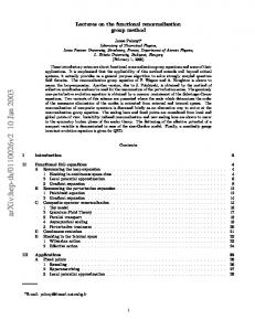
r1 (u) = 1−0.288797 u2+0.0967487 u3−0.0109959 u4 +0.000197282 u5+0.0000162077 u6 +1.37054 10−6 u7 +1.06127 10−7 u8 +5.84538 10−9 u9 −1.50021 10−10 u10 −1.19821 10−10 u11 −2.52931 10−11 u12 −3.93584 10−12 u13 −4.90717 10−13 u14 −4.49154 10−14 u15 −1.21758 10−15 u16 +6.77579 10−16 u17 +2.11465 10−16 u18 +4.19348 10−17 u19 +6.49482 10−18 u20 +7.78044 10−19 u21 +5.52691 10−20 u22 −4.37557 10−21 u23 −2.72231 10−21 u24 −6.74331 10−22 u25 + O(u26 ) . (4.16) At second order in ǫ, we have to solve 0 = r2 (u) − 4ζ2 r1 (u) − 4ζ1 r2 (u) + uζ2 r1′ (u) + uζ1 r2′ (u) +r1′′ (u)r2′′ (u) − r1′′ (0)r2′′ (u) − r1′′ (u)r2′′ (0) 1 1 + (r1′′ (u) − r1′′ (0)) r1′′′ (u)2 − r1′′ (u)r1′′′ (0+ )2 (4.17) 2 2 0 = r2 (0) , (4.18) ˜ where the last equation reflects our choice of R(0) = ǫ. Note that to solve the 2-loop order equation, one has to feed in the solution at 1-loop order, both the Taylor-expansion about 0 and the numerically obtained solution for larger u. Again ζ2 is determined from the condition that the solution decays at infinity. Following the same procedure as at 1-loop order, we find ζ2 = 0.006858(1) .

(4.19)

13 The function r2 is plotted on figure 11. The Taylor-expansion up to order 25 about 0 reads r2 (u) = −0.0604942 u2+0.0345276 u3−0.00628098 u4 +0.000239628 u5+0.000019823 u6 +1.42202 10−6 u7 +5.17941 10−8 u8 −8.64456 10−9 u9 −2.72755 10−9 u10 −4.78607 10−10 u11 −6.23531 10−11 u12 −5.49541 10−12 u13 −8.78473 10−15 u14 +1.30232 10−13 u15 +3.60568 10−14 u16 +6.7239 10−15 u17 +9.51299 10−16 u18 +9.06111 10−17 u19 −9.06201 10−20 u20 −2.59561 10−18 u21 −7.67911 10−19 u22 −1.53922 10−19 u23 −2.36569 10−20 u24 −4.42973 10−21 u25 + O(u26 ) . (4.20) One observes that ζSR is necessarily bounded from above by ǫ/4 as no SR solution can cross this value (to any order) without exploding. This reflect the exact bound for SR disorder θ < d/2, which simply means that optimization of energy must lower energy fluctuations compared to a simple sum of random numbers. Equality is obtained for the trivial constant ˜ ˜ eigenmode R(u) = R(0) corresponding to ζ = ǫ/4, associated to the fluctuation of the zero mode of the random potential. We can now discuss our results for the roughness exponent. These are summarized in Table 12 and compared to numerical simulations in d = 3, 2 and the exact result for the directed polymer in d = 1. A first observation is that the corrections compared to the 1-loop result have the correct sign and, further, that they improve the precision of the 1-loop result. Given the difficulties associated with this theory, this is a significant achievement. Second, the error bars given in Table 12 are estimated as half the 2-loop contribution, which should not be taken too literally, as it is difficult to obtain a good precision from only two terms of the series and no currently available information about the large order behavior of this novel ǫ-expansion. Third, one may try to improve the precision using the exact result ζ = 2/3 in d = 1. Estimating the third order correction in the three possible Pade’s in order to match ζ = 2/3 for ǫ = 3, we obtain consistently the values quoted in the fourth column of Table 12. We hope that these predictions can be tested in higher precision numerics soon. B.

Non-periodic systems: random field disorder

Let us first recall that at the level of the bare model the static ˜ random field disorder correlator obeys R(u) ∼ −˜ σ |u| at large |u| [46, 70], where σ ˜ = (ǫI˜1 )σ is proportional to the amplitude of the random field. If one studies the large u behavior in the FRG equation (3.43) one clearly sees that the non-linear terms do not contribute, thus one has: −m∂m σ ˜ = (ǫ − 3ζ)˜ σ.

(4.21)

Thus for a RF fixed point to exist, the O(ǫ2 ) correction to ζ has to vanish. ζRF = ǫ/3 .

(4.22)

This will presumably hold to all orders. Indeed it is clear that if there is a similar β-function to any order, since each R carries at least two derivatives and at least one must be evaluated at u 6= 0, the sum of all non-linear terms to a given finite order decreases at least as R′′ (u) ∼ 1/u. (This does not strictly excludes that summing up all orders may yield a slower decay, although it appears far fetched and does not occur in the non-perturbative large-N limit.) The above value of ζ ensures that mǫ R(u) ∼ −σ|u| in the effective action, i.e. non-renormalization of σ. Note that this argument based on long-range large u behavior is a priori valid for any λ. Since it is made on the R equation (no such argument can be made on the equation for ∆) it uses the property of potentiality. However, from (3.46) with ζ = ǫ/3 one sees that λ 6= 1 is incompatible with the existence of a fixed point, even of a fixed point with a supercusp. Thus, the only way to satisfy potentiality for the static random field problem seems to have σ unrenormalized, ζ = ǫ/3 and λ = 1 (the previous discussion of potentiality in Section III.D assumed short-range disorder). This must be contrasted with the theory of depinning, where we found that: ǫ ζdep = (1 + 0.14331ǫ) (4.23) 3 following from λdep = −1 in (3.47). Since in that case the RG-flow is non-potential, it is clear that no similar argument as above exists to protect the value ζ = ǫ/3. (The force correlator is short range). The conjecture of [57] thus appears rather unphysical in that respect. 1. Fixed-point function

We first study the fixed-point equation for ˜ ˜ ′′ (u) = ǫ y(u) ∆(u) = −R 3 y(0) = 1

(4.24) (4.25)

and later use the rescaling freedom to tune the solution to the correct value of σ at large scale u. The 2-loop FRG equation (3.47) becomes (λ = 1): 1 (4.26) 0 = (uy)′ − ((y − 1)2 )′′  2  ǫ 1 ′2 1 + (y (y − 1))′′ − y ′ (0+ )2 y ′′ . 3 2 2 One can then integrate once with respect to u: 0 = uy − y ′ (y − 1)   ǫ 1 ′2 1 ′ + 2 ′ ′ + (y (y − 1)) − y (0 ) y . 3 2 2

(4.27)

There is no integration constant here because the second line precisely vanishes at u = 0+ (absence of supercusp).

14 ζeq d=3 d=2 d=1

one loop two loop 0.208 0.417 0.625

0.215 0.444 0.687

estimate 0.215 ± 0.004 0.444 ± 0.015 0.687 ± 0.03

improved estimate simulation and exact 0.214 0.438 2/3

0.22 ± 0.01 [82] 0.41 ± 0.01 [82] 2/3 [83]

FIG. 12: First column: Exponents obtained by setting ǫ = 4 − d in the 1-loop result. Second column: Exponents obtained by setting ǫ = 4 − d in the 2-loop result. Third column: errors bars are estimated as half the 2-loop contribution. Fourth column: Improved estimates using the exact result ζeq = 2/3 in d = 1 (see text).

The 1-loop solution involves the first line only. Dividing by y and integrating over u yields: u2 = y1 − 1 − ln y1 , 2

(4.28)

i.e. an implicit equation for y, which defines y = y1 (u). It satisfies y1 (0) = 1 , 2 y1′′ (0+ ) = , 3

y1′ (0+ ) = −1

1 y1′′′ (0+ ) = − . 6

(4.29)

We can put the 2-loop solution under a similar form. Making the ansatz u2 ǫ = y − 1 − ln y − F (y) , 2 3

(4.30)

one obtains F (y(¯ u)) =

1 2

Z

0

u ¯


′ du ′2 y (y − 1) − y . y

(4.31)

At this order, one can replace y by y1 , i.e. use uy = y ′ (y − 1) to eliminate y ′ . This gives, changing variables from u to y:   Z 1 d y 2 [u(y)]2 1 y¯ −y . (4.32) dy F (¯ y) = 2 1 y dy y−1 The last term in the brackets is easily integrated. For the remaining terms, we integrate by part and use (4.30) to replace u2 /2 by y − 1 − ln y: Z y¯ y − 1 − ln y y¯ (¯ y − 1 − ln y¯) 1 F (¯ y) = dy + − ln y¯ . y−1 y¯ − 1 2 1 (4.33) This yields the final result y ln y 1 − ln y + Li2 (1 − y) (4.34) 1−y 2 Z 0 ∞ ln(1 − t) X z k . (4.35) = Li2 (z) := dt t k2 z F (y) = 2y − 1 +

k=1

We find: 13 2 F (y) = (y − 1)2 − (y − 1)3 + O((y − 1)4 ) 3 36

(4.36)

has a quadratic behavior around y = 1, similar to the 1-loop result, and corrects the value of the cusp.

2. Universal amplitude

Since we know the exact fixed point function up to a scale factor, we can now fix the scale by fitting the exact large |u| behavior to R(u) ∼ −σ|u| where σ is the amplitude of the random field. The general fixed point solution reads: ǫ ˜ ∆(u) = ξ 2 y(u/ξ) , (4.37) 3 where ξ can be related to σ as: Z ∞ ǫ ˜ du ∆(u) = ξ 3 Iy . σ ˜= 3 0

(4.38)

We need Iy =

Z

∞

du y(u) =

0

Z

1

dy u(y)

0

= γ1 + ǫγ2 Z 1 p γ1 = dy 2(y − 1 − ln y)

(4.39)

0

= 0.775304245188 Z 1 F (y) γ2 = − dy p 3 2(y − 1 − ln y) 0 = −0.13945524 .

(4.40)

(4.41)

One can now express ˜ ∗ (0) = ǫ ξ 2 = ǫ ∆ 3 3



3˜ σ ǫ

2/3

Iy−2/3

(4.42)

and thus compute, using (4.4) the universal amplitude (4.3) associated to the mode q = 0 in presence of a confining mass:  ǫ  31 2 1 2 (γ1 + ǫγ2 )− 3 (ǫI˜1 )− 3 (4.43) c˜(d) = σ 3 3  − 31  ǫ  13 ǫΓ( 2ǫ ) 2 −2 = (γ1 + ǫγ2 ) 3 σ3 , 3 (4π)d/2

˜ and σ where one has restored the factors ǫI˜1 absorbed in ∆ ˜. Expanding all factors in a series of ǫ one finds:

c˜(d) = ǫ1/3 (3.52459 − 0.725079ǫ + O(ǫ2 ))σ 2/3 , (4.44) The lowest order was obtained in Ref. [70] and we have obtained here the next order corrections. It is interesting to compare our result with the exact result in d = 0, which is [69]: c˜(d = 0) = 1.05423856519 . . .σ 2/3 .

(4.45)

15 While the simple extrapolation setting ǫ = 4 of (4.44) to one loop c˜(d = 0) = 5.59σ 2/3 is very far off, to two loop it gives c˜(d = 0) = 0.99σ 2/3 , surprisingly close to the exact result. It was noted in Ref. [70] that extrapolation of the 1-loop result could be considerably improved by not expanding (4.43) in ǫ but instead directly setting ǫ = 4 (with γ2 = 0) in (4.43). That gives c˜1 (d = 0) = 0.821σ 2/3 , an underestimate already reasonably close from the exact result. We extend this pro−2/3 cedure to two loop by truncating the ǫ expansion of Iy to second order in (4.43), and then set ǫ = 4. This yields c˜2 (d = 0) = 1.22σ 2/3 , and the exact result is then halfway between c˜1 (d = 0) and c˜2 (d = 0). To summarize, our 2-loop corrections (4.44) have the correct sign and order of magnitude to improve the agreement with the exact result in d = 0. The universal amplitude for the massless case (4.7) (or q ≫ m) is obtained from (4.8) with b = −1/3 from Section VI as:   1 c(d) = c˜(d) 1 − ǫ + O(ǫ2 ) 3   1/3 3.52459 − 1.89994ǫ + O(ǫ2 ) σ 2/3 , (4.46) =ǫ and writing c(d) = c˜(d)/(1 + 13 ǫ) should provide a reasonable extrapolation to low dimensions. Finally, we recall that for random field disorder, this coefficient is different for different large scale boundary conditions. The result for periodic boundary conditions can be obtained from formula (4.10). In Ref. [70], the 1-loop result was compared to the result of the Gaussian Variational Method (GVM). It is instructive to pursue this comparison to two loops. We get from [70]:  ǫ  13  ǫΓ( ǫ ) − 31 2 1 2 3 c˜GVM (d) = 2 ǫ σ d/2 π 1 − 12 (4π)

where in the last line we have inserted ζ = ǫ/3 and performed the ǫ expansion. Thus one finds, quite generally that bvar = 3b/4. As noted in [70] to one loop the FRG and the GVM give rather close amplitudes (differing by about 5 per cent). We see here that to two loop, i.e. next order in ǫ, the difference increases. Finally, cGVM (d) = ǫ1/3 (3.69054 − 1.81686ǫ + O(ǫ2 ))σ 2/3 and the coefficient remains rather close to the one in (4.46). C. Generic long range fixed points There is a family of fixed points such that

ǫ . 2(1 + γ)

0.6 0.4 0.2 1

2

3

4

FIG. 13: The fixed-point function y1 (u) at 1-loop order for nonperiodic disorder.

These fixed points where found for infinite N in any d in Ref. [36, 72] (we use the same notations). They were studied to first order in ǫ for any N in [47], and argued to be stable only for γ < γ ∗ (d) the value of the crossover to short range identified in [47] as ζSR = ζLR (γ ∗ (d)). Here, we have not studied these fixed points in detail but we note that the 2-loop corrections do not change ζ, by the same discussion as for the random field case γ = 1/2. They will however affect the amplitudes. D. Periodic systems

For periodic R(u) as e.g. CDW there is another fixed point of (3.43). It is sufficient to study the case where the period is set to unity, all other cases are easily obtained using the reparametrization invariance of equation (4.11). No rescaling is possible in that direction, and thus the roughness exponent is ζ =0.

(4.49)

(4.50)

(4.51)

The fixed-point function is then periodic, and can in the interval [0, 1] be expanded in a Taylor-series in u(1 − u). Even more, the ansatz
˜ R(u) = (a1 ǫ + a2 ǫ2 + . . . ) + b1 ǫ + b2 ǫ2 + . . . u2 (1 − u)2 (4.52) allows to satisfy the fixed-point equation (3.43) to order ǫ2 and will presumably work to all orders. For a more general case of this see Ref. [68]. To gain insight into the more general case, let us write the fixed point for (3.43) with arbitrary λ: ˜ ∗ (u) = R

associated with ζ=

0.8

1. Fixed point function

(4.47)

= ǫ1/3 (3.69054 − 0.894223ǫ + O(ǫ2 ))σ 2/3    cGVM (d) ǫ − 2ζ π (ǫ − 2ζ) /2 ǫ − 2ζ 1− = 1− c˜GVM (d) 2 4 sin(π(ǫ − 2ζ)/2) ǫ 2 (4.48) = 1 − + O(ǫ ) 4

˜ R(u) ∼ |u|2(1−γ)

1

ǫ ǫ2 + (3 − 2λ) 2592 7776 ǫ2 u(1 − u) +(λ − 1) 432   ǫ2 ǫ u2 (1 − u)2 . + − 72 108

(4.53)

16 One can see on this solution that λ = 1 is the only value which avoids the appearance at two loops of the supercusp, ˜ i.e. a cusp in the potential correlator R(u) rather than in the ˜ force correlator ∆(u). The same discussion can be made on the the flow equation ˜ of ∆(u) by taking two derivatives of (3.43). One finds that there is a priori an unstable direction corresponding to a uni˜ ˜ form shift in ∆(u) → ∆(u) + cst. While this is natural in e.g. depinning, it is here forbidden by the potential nature of the problem which requires Z

1

˜ du ∆(u) =0,

(4.54)

0

since in a potential environment, the integral of the force over one period must vanish. This is indeed satisfied for the fixed ˜ point for ∆(u) ˜ ∗ (u) = −R ˜ ∗′′ (u) ∆     λ−1 ǫ ǫ2 ǫ2 ǫ 1+ − u(1 − u) + + = 36 54 4 6 9 (4.55) only if λ = 1: Z

1

0

2 ˜ ∗ (u) = ǫ (λ − 1) du ∆ 216

(4.56)

The values for depinning are obtained by setting λ = −1: in that case, the problem becomes non-potential at large scales. 2. Universal amplitude

This fixed point implies for the amplitude of the zero mode in presence of an harmonic well, defined in (4.3), using (4.4): (4π)d/2 c˜(d) = ǫΓ( 2ǫ )



 ǫ ǫ2 3 + + O(ǫ ) 36 54

= 2.19325ǫ − 0.680427ǫ2 + O(ǫ3 )

(4.57)

(4.59)

Note that we prove in Section (VI) that this amplitude is independent of large scale boundary conditions, and is thus identical for e.g. periodic boundary conditions and in presence of a mass. As can be seen from (4.10) this is a consequence of ζ being zero. This can be compared to the GVM method [26, 28]:   d d (4.60) cGVM (d) = (4 − d)2d−3 π 2 −2 Γ 2 = 2ǫ − 2.9538ǫ2 + O(ǫ3 )

c1 (d = 3) = 2π/9 = 0.6981 cGVM (d = 3) = 1/2 .

(4.61)

(4.62) (4.63)

Including the 2-loop ǫ2 /108 term now gives c2 (d = 3) = 0.4654 and c2 (d = 3) = 0.5235 for the two Pades respectively. This type of extrapolation makes the GVM and FRG predictions get closer when including the 2-loop corrections. On the other hand, comparison of (4.59) and (4.61) suggests that c(d) > cGVM (d). This is in reasonable agreement with the numerical results of Middleton et al. [84]. They obtained good evidence for the existence of the Bragg glass (i.e. its stability with respect to topological defects predicted in [26, 28]). They measure directly the correlation (4.7) and obtain strong evidence for the behavior (4.58) (as well as the correct correction to scaling behavior) with 2c(d = 3) ≈ 1.04 ,

(4.64)

(their amplitude A is twice our c(d)) which lies in between the GVM and the 1-loop FRG. (More precisely two different discretizations gave 2c(d = 3) = 1.01 ± 0.04 and 2c(d = 3) = 1.08 ± 0.05). Another interesting observable is the slow growth of displacements characteristic of the Bragg glass: (ux − u0 )2 = A˜d ln |x|

In the other limit m ≪ q one obtains the amplitude (using b = −1 from Section VI):   (4π)d/2 ǫ ǫ2 3 c(d) = − + O(ǫ ) (4.58) ǫΓ( 2ǫ ) 36 108 = 2.19325ǫ − 2.87367ǫ2 + O(ǫ3 )

with coefficients surprisingly close to the ǫ-expansion. It is interesting to compare predictions in d = 3. We recall that we are studying a problem where the period is unity, the general case being obtained by a trivial rescaling in u. Since (4.59) has a poor behavior (and so does (4.61) which resums into (4.60)), it is better to use instead (4.58). It was indeed noted in [26, 28] that the improved 1-loop prediction c1 (d = 3) obtained by setting ǫ = 1 and ignoring the ǫ2 /108 term in (4.58) yields a value rather close to the prediction of the GVM:

(4.65)

at large x. Performing the momentum integral from (4.7), one obtains: 4 c(d) (4π)d/2 Γ(d/2)   4 sin(πǫ/2) ǫ ǫ2 3 = − + O(ǫ ) πǫ(1 − 2ǫ ) 36 108

A˜d =

(4.66)

If one expands each factor in ǫ it yields: ǫ2 ǫ + + O(ǫ3 ) A˜d = 18 108

(4.67)

For comparison, the GVM gives ǫ A˜d,GVM = 2 . 2π

(4.68)

Here extrapolation directly setting ǫ = 1 in (4.67) looks possible, and yields A˜3 = 0.0556 to one loop increasing to A˜3 = 0.0648 to two loop. On the other hand, setting ǫ = 1

17 in (4.66) yields instead A˜3 = 0.0707 to one loop decreasing to A˜3 = 0.047 at two loops. The GVM gives the result A3,GVM = 0.0507. Another interesting observable is: w2 = Bd ln L 2  Z Z 1 1 2 2 , u − ux w = d L x x Ld x

(4.69) (4.70)

where L is the linear system size. In Ref. [84] it was assumed that Bd = A˜d /2 thus in d = 3, B3 = c(3)/(2π 2 ) yielding a value of c(d) consistent with the direct measurement of this quantity [104]. This was also done in [85] where it was deduced from a measurement of Bd that 0.98 < 2c(d = 3) < 1.11 [105]. Although this is a reasonable approximation, it is not exact. Indeed the quantity Bd , contrary to c(d), depends on the (large scale) boundary conditions. It is of course universal, since it does not depend on small scale details. Its value can be computed e.g. for periodic boundary conditions and pinned zero mode, and depends on the whole finite size scaling function (4.9) computed in Section VI: X w2 = c(d) q −(d+2ζ gd (qL) (4.71) q6=0

As shown recently, w2 fluctuates from sample to sample and the full distribution P (w2 ) averaged over disorder realizations was computed for the depinning problem [86, 87].

and thus the β-function is given by (3.43) with: (α)

X → X (α) := =

(α)

2 ǫ(2IA − (I1 )2 ) (α)

(ǫI1 )2 α

1

(See appendix F of Ref. [67]). And of course the relation ˜ is identical except that ǫI˜1 must be re(3.42) between R and R (α) ˜ placed by ǫI1 . Since X (α) is finite, the β-function is finite; this is of course necessary for the theory to be renormalizable. For the cases of interest α = 1 and α = 2, we find X (2) = 1 X (1) = 4 ln 2 .

(4.79) (4.80)

The exponent ζ (as a function of ǫ) and the fixed point function is thus changed only at two loops. Let us now give the results in the cases of interest: 1. Random bond disorder

The solution of (3.43) with X → X (α) can be written, to second order in ǫ as: ˜ R(u) = ǫ r1 (u) + ǫ2 X (α) r2 (u) + . . . 2

ζ = ǫ ζ1 + ǫ X

E. Long range elasticity

α

dt 1 + t 2 − (1 + t) 2 α + ψ(α) − ψ( ) α t 2 (1 + t) 2 0 + O(ǫ) . (4.78) Z

(α)

ζ2 + . . . ,

(4.81) (4.82)

Let us now consider the case of long range elasticity. There are physical systems where the elastic energy does not scale with the square of the wave-vector q as Eelastic ∼ q 2 but as Eelastic ∼ |q|α . In this situation, the upper critical dimension is dc = 2α and we define:

since the equation (4.17) for r2 (u) is linear. Thus one has for any α:

ǫ := 2α − d .

ζ = 0.20829806(3)ǫ + 0.0190114(3)ǫ2 ǫ=2−d

(4.72)

The most interesting case, a priori relevant to model a contact line is α = 1, thus dc = 2. For calculational convenience, we choose the elastic energy to be α 2

Eelastic ∼ (q 2 + m2 ) .

(4.73)

This changes the free correlation to: Gab (q) = δab

(q 2

T α . + m2 ) 2

(4.74)

The energy exponent in that case is: θ = α − d + 2ζ .

(4.75)

The changes are very similar to the case of Ref. [67] so we summarize them here only briefly. The β-function is still given by (3.40) but with the integrals replaced by: Z Z 2 1 (α) −ǫ Γ(ǫ/2) =m I1 = e−q (4.76) 2 + m2 )α (q Γ(α) q q Z 1 (α) IA = α 2 + m2 ) α 2 (q 2 + m2 )α ((q + q )2 + m2 ) 2 (q 1 2 q1 ,q2 2 1 (4.77)

ζ = 0.20829806(3)ǫ+ 0.006858(1)X (α)ǫ2 + O(ǫ3 ) . (4.83) For the case of most interest α = 1, X (1) = 4 ln 2 one finds:

(4.84)

and θ = 2ζ. It would thus be interesting to perform numerical simulations in d = 1 for the directed polymer with LR elasticity. This would be another non trivial test of the 2-loop corrections. The 1-loop prediction is ζ = 0.208, significantly smaller than the roughness for SR elasticity ζ = 2/3. The naive 2-loop result is (setting ǫ = 1), ζ ≈ 0.227 ± 0.01. Error bars are estimated by half the difference between the 1loop and 2-loop results. Note that the bound θ < d/2 implies ζ < 1/4 in d = 1, already rather close to the 2-loop result. 2. Random field disorder

The exponent is still ζ=

ǫ 3

(4.85)

and was indeed measured in experiments on an equilibrium contact line [30]. It would be of interest to measure the universal distributions there, such as the one defined in [86, 87].

18 The fixed point function is given by (4.30) and (4.34) upon replacing F (y) → X (α) F (y). The amplitude of the zero mode in a well c(d) is now given by: c˜(d) = σ 2/3

 ǫ 1/3  3

γ1 + ǫX (α) γ2

−2/3

(α)

(ǫI˜1 )−1/3 (4.86)

and the amplitude of the massless propagator c(d) = c˜(d)(1 + bα ǫ) .

(4.87)

where bα is given in (6.14) setting ζ1 = 1/3. 3. Periodic disorder

The fixed point becomes: ˜ ∗ (u) = −R ˜ ∗′′ (u) ∆   ǫ ǫ2 (α) ǫ2 (α) ǫ = u(1 − u) . (4.88) + X − + X 36 54 6 9 For the periodic case, the universal amplitude reads:   ǫ2 (α) (4π)d/2 ǫ 3 + X + O(ǫ ) c˜(d) = Γ(α) ǫΓ( 2ǫ ) 36 54

(4.89)

and c(d) = c˜(d)(1 + bα ǫ) .

(4.90)

Setting ζ1 = 0 in (6.14) yields A˜d =

4 (4π)d/2 Γ(d/2)

c(d) .

(4.91)

Using ǫ = 2α − d, this gives 4X (α) + 3(γ + ψ(α)) + 6bα 2 1 ǫ+ ǫ , A˜d = 18 108

(4.92)

which in the case of α = 1 takes the simple form 1 4X (α) + 6bα 2 A˜1 = ǫ+ ǫ . 18 108

V.

(4.93)

LIFTING AMBIGUITIES IN NON-ANALYTIC THEORY

A. Summary of possible methods As we have seen above ambiguities arise in computing the effective action at the level of 2-loop diagrams if one uses a non-analytic action. One can see that these arise even at the 1loop level for correlations (see below Section VI). To resolve this issue, our strategy has been to use physics as a guide and require the theory to be renormalizable, potential and without supercusp. This pointed to a specific assignment of values to the “anomalous” graphs. The physical properties of the ensuing theory, studied in the previous section, were found to be quite reasonable. Of course, one would like to have a better, more detailed justification of the used “prescription”. Although we do not know at present of a derivation of this theory

from first principles, we have developed a set of observations and a number of rather natural and compelling “rules” which all lead to the same theory. We describe below our successful efforts in that direction as well as some unsuccessful ones, which illustrate the difficulty of the problem. A number of approaches can be explored to lift the ambiguities in the non-analytic theory. We here give a list; some of the methods will be detailed in the forthcoming sections. 1) Non-zero temperature: At T > 0 previous Wilson 1loop FRG analysis[58, 59, 70, 88] found that the effective action remains analytic in a boundary layer u ∼ T˜. However, since the rescaled temperature (2.24) flows to zero as T˜ ∼ mθ as m → 0 (temperature being formally irrelevant) all (even) derivatives of R(u) higher than second grow unboundedly as m → 0, for instance R′′′′ (0) ∼ R∗′′′ (0+ )2 /T˜ (in terms of the zero temperature fixed point function). On a qualitative level one can thus see how finite T diagrams such as E in Fig. 3 yielding ∼ T R′′′′ (0)R′′ (u) → R∗′′′ (0+ )2 R′′ (u)

(5.1)

can build up “anomalous” terms in the β-function, hence confirming what is found here[70]. However, correctly and quantitatively accounting for higher loops is a non-trivial problem as stronger blow-up in 1/T˜ k seem to arise. In fact each new loop brings two derivatives and a propagator, hence an additional factor 1/T˜. Despite some recent progress, a quantitative finite-temperature approach which would reproduce and justify the present ǫ expansion has proved difficult[74, 75]. Not only for technical reasons, as methods using exact RG where found to be appropriate, but also for physical reasons, as an extension to non-zero T must also handle low-lying thermal excitations in the system (e.g. droplets). A theory from first principles at T > 0 is thus presently not available and will not be further addressed here. All other methods use a nonanalytic action. 2) Exact RG: Exact RG methods directly at T = 0 have been studied to one loop [70, 89] and two loops[71, 90]. Although it does yield interesting insights into the way to handle ambiguities (see below), and confirm the present results, it suffers from basically the same problems as described here. 3) Direct evaluation of non-analytic averages: In this approach one attempts a direct evaluation of non-analytic averages (e.g. in fully saturated diagrams). For instance, expanding at each vertex the disorder R(uxa − uxb ) in powers of |uxa − uxb | using the proper non-analytic Taylor expansion: R′′ (u) = R′′ (0) + R′′′ (0+ )|u| + R′′′′ (0+ )u2 + . . .

(5.2)

one can try to compute directly all averages in vertex functions and correlations. After performing a few Wick contractions one typically ends up with averages involving sign functions or delta functions. These can be computed in principle using the free Gaussian measure. For instance, using formulae such as: ! huvi0 2 hsgn(u)sgn(v)i0 = asin p . (5.3) π huui0 hvvi0

19 Although promising at first sight, the results are disappointing. Averages over the thermal measure involve many changes of signs which kill all interesting divergences indicating that some physics is missing. The method, briefly described in Appendix B is thus not developed further. A dynamical version of this method which is similar in spirit [66, 67], did work for depinning, although there it simply identified with another method used below, the background field (which, for depinning is uxt → vt + uxt see below). 4) Calculation of Γ(u) with excluded vertices and symmetrization: A valid, general and useful observation (not limited to this method) is that if one uses the excluded vertex 1 X R(ua − ub ) , 2T 2

hui W (u)i = (5.4)

a6=b

then all Wick contractions can be performed without ambiguities. The excluded vertex is as good as the non-excluded one since one can always add a constant −nR(0) to the action of the model (2.2). Thus one can compute without any ambiguity the effective action Γ(u) for an “off-diagonal” field configuration uax

such that uax 6= ubx

for all a 6= b ,

(5.5)

since then no vertex is ever evaluated at u = 0. The drawback is that one ends up with expressions containing terms such as X R′′ (ua − ub )R′′′ (ua − ub )R′′′ (ub − uc ) , (5.6) a6=b,a6=c

which superficially looks like a three replica term, but due to the exclusions, may in fact contain a 2-replica part which can in principle be recovered from the above by adding appropriate diagonal terms, using that p-replica parts are properly defined as free replica sums e.g. from a cumulant expansion. The 2-replica part of (5.6) thus naively is X − R′′ (0)R′′′ (0)R′′′ (ua − uc ) ac

+

X ab

R′′ (ua − ub )R′′′ (ua − ub )R′′′ (0)

If one renounces to the projection onto 2-replica terms one can, in a certain sense, obtain renormalizability properties. This generates an infinite number of different replica sums and seems to be not promising, too. It is described in Appendix F. We now come to methods which were found to work, and which will be described in detail in the next section. In all of them one performs the Wick contractions in some given order (the order hopefully does not matter) and uses at each stage some properties. The fact that one can order the Wick contractions stems from the identity, which we recall, for any set of mutually correlated Gaussian variables ui :

(5.7)

and one is again faced with the problem of assigning a value to R′′′ (0). The calculation with excluded vertices thus yields a sum of p-replica terms with p ≥ 2 and to project them onto the needed 2-replica part, one may need to continue these expressions to coinciding arguments ua = ub . The symmetrization method attempts to do that in the most “natural” way. Using the permutation symmetry over replicas and the hypothesis of no supercusp yields a rather systematic method of continuation. Surprisingly, it fails to yield a renormalizable theory at two loops. We identified some difference with methods which do work, but the precise reason for the failure in terms of continuity properties remains unclear. It may thus be that there is a way to make this method work but we have not found it. Being interesting in spirit this method is reported in some details in Appendix A.

X j



hui uj i ∂uj W (u)

(5.8)

under very little analyticity assumption for W (u), which can even be a distribution. At each stage one can either use excluded or non-excluded vertices as is found more convenient. 5) Elimination of sloops: We found another method, which seems rather compelling, to determine the 2-replica part of terms such as (5.6). It starts, as the previous one, by computing (unambiguously) diagrams with the excluded vertices. Then instead of symmetrization, one uses identities derived from the fact that diagrams with free replica sums and which contain sloops cannot appear in a T = 0 theory and can thus be set to zero. Further contracting such diagrams generates a set of identities which, remarkably, is sufficient to obtain unambiguously the 2-replica projection without any further assumption. It works very nicely and produces a renormalizable theory, as we have checked up to three loops. In some sense, it uses in a non-trivial way the constraint that we are working with a true T = 0 theory. This method is detailed below. 6) Background field method: This method is similar to method number 3 except that the vertex R(u) at point x is evaluated at the field uax = ua + δuax , then expanded in δuax , which then are contracted in some order. This amounts to compute the effective action in presence of a uniform background field which satisfies (5.5). Thanks to this uniform background and upon some rather weak assumptions, the ambiguities seem to disappear. The method is explained below. 7) Recursive construction: An efficient method is to construct diagrams recursively. The idea is to identify in a first step parts of the diagram, which can be computed without ambiguity. This is in general the 1-loop chain-diagram (3.1). In a second step, one treats the already calculated sub-diagrams as effective vertices. In general, these vertices have the same analyticity properties, namely are derivable twice, and then have a cusp. (Compare R(u) with (R′′ (u)−R′′ (0))R′′′ (u)2 − R′′ (u)R′′′ (0+ )2 ). By construction, this method ensures renormalizability, at least as long as there is only one possible path. However it is not more general than the demand of renormalizability diagram by diagram, discussed below. 8) Renormalizability diagram by diagram: In Section III we have used a global renormalizability requirement: The 1loop repeated counter-term being non-ambiguous one could

20 fix all ambiguities of the divergent 2-loop corrections. However, as will be discussed in [73], this global constraint appears insufficient at three loops to fix all ambiguities. Fortunately, one notes that renormalizability even gives a stronger constraint, namely renormalizability diagram by diagram. The idea goes back to formal proofs of perturbative renormalizability in field-theory, see e.g. [91, 92, 93, 94, 95, 96, 97, 98]. These methods define a subtraction operator R. Graphically it can be constructed by drawing a box around each sub-divergence, which leads to a “forest” or “nest” of subdiagrams (the counter-terms in the usual language), which have to be subtracted, rendering the diagram “finite”. The advantage of this procedure is that it explicitly assigns all counter-terms to a given diagram, which finally yields a proof of perturbative renormalizability. If we demand that this proof goes through for the functional renormalization group, the counter-terms must necessarily have the same functional dependence on R(u) as the diagram itself. In general, the counter-terms are less ambiguous, and this procedure can thus be used to lift ambiguities in the calculation of the diagram itself. By construction this procedure is very similar to the recursive construction discussed under point 7. It has some limitations though. Indeed, if one applies this procedure to the 3-loop calculation, one finds that it renders unique all but one ambiguous diagram, namely ,

(5.9)

which has no subdivergence, thus there are no counter-terms, which could lift the ambiguities. Thus this diagram must be computed directly and we found that it can be obtained unambiguously by the sloop elimination method[73]. 9) Reparametrization invariance: From standard field theory, one knows that renormalization group functions are not unique, but depend on the renormalization scheme. Only critical exponents are unique. This is reflected in the freedom to reparametrize the coupling constant g according g −→ g˜(g) where g˜(g) is a smooth function, which has to be invertible in the domain of validity of the RG β-function. Here we have chosen a scheme, namely defining R(u) from the exact zero momentum effective action, using dimensional regularization, and a mass. One could explore the freedom in performing reparametrization. In the functional RG framework, reparametrizations are also functional, of the form ˆ ˆ R(u) −→ R(u) = R[R](u) .

B(R, R) = δ (1,1) R. One can convince oneself, that by choosing the correct amplitude, one can eliminate all contributions of class A, in favor of contributions of class B. Details can be found in [73]. Apart from methods 3 and 4 which did not work for reasons which remain to be better understood, methods 2,5,6,7,8,9 were all found to give consistent result, making us confident that the resulting theory is sufficiently constrained by general arguments (such as renormalizability) to be uniquely identified. Let us now turn to actual calculations using these methods.

B. Calculation using the sloop elimination method 1. Unambiguous diagrammatics

Let us redo the calculation of Section III B using excluded vertices. From now on we use sometimes the short-hand notations uab = ua − ub

Rab = R(ua − ub )

ˆ Of course the new function R(u) does not have the same meaning as R(u). Perturbatively this reads ˆ R(u) −→ R(u) = R(u) + B(R, R)(u) + O(R3 ) , (5.11) where B(R, R) is a functional of R. For consistency, one has to demand that B(R, R) has the same analyticity proper˜ = R ˜ ∗ , i.e. B(R, R) ties as R, at least at the fixed point R should as R be twice differentiable and then have a cusp. A specifically useful candidate is the 1-loop counter-term

,

a b uab x = ux − ux (p)

Rab = R(p) (ua − ub )

(5.12)

whenever confusion is not possible. The resulting diagrammatics looks very different from the usual unexcluded one. When making all four Wick contractions of the 2-loop diagrams A, B and C in Fig. 6 between three unsplitted vertices one now excludes all diagrams with saturated vertices, but instead has to allow for more than two connected components and for sloops. The splitted excluded diagrams corresponding to classes A, B and C are given in Fig. 14. There is an additional multiplicative coefficient 1/(m1 !m2 !m3 !m4 !) in the combinatorics for each pair of unsplitted vertices (say ab and cd) linked by an internal line where m1 propagators link ac, m2 link ad, m3 link bc, m2 link bd. (This is equivalent to assigning a color to each propagator). (2)

Let us denote by δΓ = − 2T1 2 δA R the 2-loop contribution of all diagrams of class A to the effective action. One finds: (2)

δA R =

hX

′′ ′′′ 2 Rab (Rab ) +

a6=b

(5.10)

,

−

1 2

1 + 2

X

′′ ′′′ ′′′ Rab Rab Rac

a6=b,a6=c

X

a6=b,a6=c,b6=c

X

a6=b,a6=c,a6=d

′′ ′′′ ′′′ Rab Rac Rbc +

3 2

i ′′ ′′′ ′′′ Rab Rac Rad IA

X

′′ ′′′ 2 Rab (Rac )

a6=b,a6=c

(5.13)

coming respectively and in the same order from graphs α, β, γ, δ+η (they are equal) and λ in Fig. 14. The only graph common to excluded and free-sum diagrammatics is α which is graph b of Fig. 7, since all the other graphs in Fig. 7 have saturated vertices.

21

α

γ

β

case), or equivalently lifting all exclusions but replacing everywhere (p)

(p)

Rab → Rab (1 − δab )

η

δ

α’

β’

γ’

(5.15)

and then expanding and selecting the 2-replica part, one finds the contributions

λ

α → R′′ (u)R′′′ (u)2 1 γ → R′′ (0)R′′′ (u)2 2 3 δ + η → − R′′ (0)R′′′ (u)2 2 β→0 λ→0.

α’’

δ’

(5.16)

Similarly in (5.14) one obtains

β’’

γ’’

δ ’’

η’’

λ’’

ν ’’

1 ′′′′ R (u)R′′ (u)2 2 1 1 β ′ → γ ′ → R′′′′ (0)R′′ (0)R′′ (u) + R′′ (0)2 R′′′′ (u) 2 4 δ ′ → −R′′′′ (0)R′′ (0)R′′ (u) − R′′ (0)R′′′′ (u)R′′ (u) . (5.17)

α′ →

We now want to perform the same projection for a nonanalytic R(u). 2. The sloop elimination method

FIG. 14: 2-loop diagrams corresponding to Larkin’s hat (top) and banana (bottom). The graph α is a 1-replica term, β, γ, δ and η are improper three replica terms and λ is an improper four replica term.

Similarly, the graphs of class B give a total contribution: " X 1 X ′′′′ ′′ ′′ 1 (2) ′′′′ ′′ ′′ δB R = Rab Rab Rab + Rab Rac Rad 2 4 a6=b a6=b,a6=c,a6=d # X X 1 ′′′′ ′′ ′′ ′′′′ ′′ ′′ + Rab Rac Rbd + Rab Rab Rac I12 4 a6=b,a6=c,b6=d

a6=b,a6=c

(5.14)

coming respectively and in the same order from graphs α′ , β ′ , γ ′ , δ ′ in Fig. 14. Again, the only graph common to excluded and free-sum diagrammatics is α′ which is graph g of Fig. 8, since all the other graphs in Fig. 8 have saturated vertices. (2) The contribution δC R of the diagrams of class C is given in Appendix C. Note that adding a tadpole does not alter the structure of the summations in the excluded-replica formalism, since a tadpole can never identify indices on different vertices. This indicates that class C does not contain a 2-replica contribution, but starts with a 3-replica contribution (times T ). This is explained in more details in Appendix D One can first check that when R(u) is analytic one recovers correctly the same result as (3.27) setting the last (anomalous) term to zero. Adding and subtracting the excluded terms in (5.13) to build free replica sums (using R′′′ (0) = 0 in that

The idea of the method is very simple. Let us consider the 1loop functional diagram (a) in Fig. 2 which contains a sloop. It is a three replica term proportional to the temperature. In a T = 0 theory such a diagram should not appear, so it can be identically set to zero: W :=

1 X ′′ ab ′′ ac R (ux )R (uy ) ≡ 0 . T2

(5.18)

abc

It is multiplied by G(x − y)2 , which we have not written. We will also omit global multiplicative numerical factors. Projecting such terms to zero at any stage of further contractions is very natural in our present calculation (and also e.g. in the exact RG approach, where terms are constructed recursively and such forbidden terms must be projected out). It is valid only when (i) the summations over replicas are free (ii) the term inside the sum is non-ambiguous. These conditions are met for any diagram with sloops, provided the vertices have at most two derivatives. (One can in fact start from vertices which either have no derivative or exactly two.) Let us illustrate the procedure on an example. We want to contract W with a third vertex R at point z, i.e. we first write the product: W

1 X 1 Rde = 4 T2 T de

X

a6=b,a6=c,de

′′ ′′ Rab Rac Rde ≡ 0 , (5.19)

where implicitly here and in the following the vertices are at points x, y, z in that order. We will contract the third vertex

22 twice, once with the first and once with the second , i.e. look at the term proportional to G(x − y)2 G(x − z)G(y − z). Note that since we will contract each vertex, we are always allowed to introduce excluded sums (clearly the diagonal terms a = b, a = c or d = e give zero, since Rab and its two lowest derivatives at a = b are field independent constants). Performing the first contraction (i.e. inserting δad − δae − δbd + δbe multiplied by the exclusion factors (1 − δab )(1 − δac)(1 − δde) yields (up to a global factor of 2): i X X 1 h ′′′ ′′ ′ ′′′ ′′ ′ R R R − R R R ab ac ae ab ac be ≡ 0 . T3 a6=b,a6=c,a6=e

a6=b,a6=c,b6=e

(5.20) Similarly, the second contraction then yields (up to a global factor of 4): X X 1 h1 ′′′ ′′′ ′′ ′′′ ′′′ ′′ Rab Rac Rae + Rab Rac Rac 2 T 2 a6=b,a6=c,a6=e a6=b,a6=c i X 1 1 X ′′′ ′′′ ′′ ′′′ ′′′ ′′ Rab Rab Rae − Rab Rac Rbc ≡ 0 . + 2 2 a6=b,b6=e

(2)

−

δA R =

,

(5.24)

where the loop with the dashed line represents the subdiagram with the sloop, i.e. the term (5.18) (with in fact the same global coefficient). The idea is of course that subtracting sloops is allowed since they formally vanish. There are other possible identities, which are descendants of other sloops. For instance a triangular sloop gives, by a similar calculation: = R′′ (0)

X a6=b

+

X

a6=b,b6=c

′′′ 2 (Rab ) +

X

′′′ ′′′ R′′ (0)Rab Rac

a6=b,a6=c

′′ ′′′ 2 Rbc (Rab )

+

X

′′′ ′′′ ′′ Rac Rbc Rcd .

a6=c,b6=c,c6=d

(5.25)

a6=b,a6=c,b6=c

(5.21)

This non-trivial identity tells us that the sum of all terms (or diagrams) generated upon contractions of diagram (a) of Fig. 2 (i.e. the 1-loop sloop-diagram equivalent to term W in (5.18)) with other vertices, must vanish. Stated differently: A sloop, as well as the sum of all its descendents vanishes. Note that this is not true for each single term, but only for the sum. A property that we request from a proper p-replica term is that upon one self contraction it gives a (p − 1)-replica term. It may also give T times a p-replica term (a sloop) but this is zero at T = 0, so we can continue to contract. Thus we have generated several non-trivial projection identities. The starting one is that the 2-replica part of (5.18) is zero, since (5.18) is a proper 3-replica term. Thus, (5.19) prior to the exclusions, is a legitimate 5-replica term, and its 4-replica part is zero. Upon contracting once we obtain that the 3-replica part of (5.20) is zero. The final contraction tells us that the 2-replica part of (5.21) is zero. This is what is meant by the symbol “≡” above and the last identity is the one we now use. Indeed compare (5.21) with (5.13). One notices that all terms apart from the first in (5.13) appear in (5.21), and with the same relative coefficients, apart from the third one of (5.13). Thus one can use (5.21) to simplify (5.13): hX i X (2) ′′ ′′′ 2 ′′ ′′′ 2 δA R = Rab (Rab ) + Rab (Rac ) IA . (5.22) a6=b

We can write diagrammatically the subtraction that has been performed

a6=b,a6=c

The function R′′′ (u)2 , which appears in the last term, is continuous at u = 0. It is thus obvious how to rewrite this expression using free summations and extract the 2-replica part h (2) δA R(u) = (R′′ (u) − R′′ (0))R′′′ (u)2 i −R′′′ (0+ )2 R′′ (u) IA , (5.23)

which coincides with the contribution of diagrams A in (3.27) with λ = 1.

(2)

This however does not prove useful to simplify δA R. Since the above method generates a large number of identities, one can wonder whether they are all compatible. We have checked a large number of examples (see the 3-loop calculations in [73]) and found no contradictions, although we have not attempted a general proof. The diagrams B and C are computed in Appendix D. One finds by the same procedure 1 ′′′′ R (u)(R′′ (u) − R′′ (0))2 2 δC R = 0 ,

δB R =

(5.26) (5.27)

confirming our earlier results in section III B 2 and III B 3. C. Background method In the background method, one computes Γ[u] to two loops for a uniform background u such that uab 6= 0 for any a 6= b. We start from 

(5.28) S[u + vx ]3 1PI Taylor expand in vx , and contract all the v fields keeping only 1PI-diagrams. This is certainly a correct formula for the uniform (i.e. zero momentum) effective action. Then one needs the small |u|-expansion of derivatives of R, i.e. (5.2) as well as R′′′ (u) = R′′′ (0+ )sign(u) + R′′′′ (0+ )u + . . . R′′′′ (u) = 2R′′′ (0+ )δ(u) + R′′′′ (0+ ) + . . . .

(5.29) (5.30)

Let us start from: X R(uab + vxab )R(ucd + vycd )R(uef + vzef ) . abcdef

We expand in v and of course in diagrams A one must handle terms involving R′′′ (0) and in diagrams B terms proportional

23 to R′′′′ (0). Let us start with diagrams A, which come from the following term in the Taylor expansion: X 

R′′′ (uab )R′′′ (ucd )R′′ (uef ) (vxab )3 (vycd )3 (vzef )2 abcdef

(5.31) Here and in the following, we will drop all combinatorial factors. Note that the expectation-values vanish at coinciding replicas so there is no need to specify the values of R′′′ (uab ) at a = b. Let us perform the first xy contraction X

 R′′′ (uab )R′′′ (uad )R′′ (uef ) (vxab )2 (vyad )2 (vzef )2 . abcef

If we now perform a second xy contraction there is a δaa term which is a sloop and thus should be discarded. The δad + δba terms build saturated vertices. However the corresponding expectation values contain

 R′′′ (uad ) (vyad ) . . . |d→a = 0 , (5.32)

which is reasonably set to zero. Thus the first two contractions have been performed with no ambiguity leading to X

 R′′′ (uab )R′′′ (uab )R′′ (uef ) (vxab )(vyab )(vzef )2 (5.33) abef

This term is no more ambiguous. Expanding as in (5.29) the potentially ambiguous part is X 

R′′′ (0+)2 (5.34) R′′ (uef ) (vxab )(vyab )(vzef )2 . abef

clearly free of any ambiguity. It yields the result (5.23). The question arises, whether the result may depend on the order. We found that when first contracting xy and xz, one reproduces the result (5.23). However when one first contracts xy and yz (in any order) one encounters a problem, if one wants to contract yz again. The intermediate result after the first two contractions is X

 R′′′ (uab )R′′′ (uad )R′′ (uaf ) (vxab )(vyad )2 (vzaf ) (5.35) abef

The next contraction between xy contains one term with a sin′′′ gle Raa . One would like to argue that this term can be set to 0. Following this procedure however leads to problems. We therefore adopt the rule, that whenever one arrives at a single ′′′ Raa , one has to stop, and search for a different path. Note that this equivalently applies to the recursive constructions method. In 2-loop order, one can always find a path, which is unambiguous. It seems to fail at 3-loop order; at least we have not yet been able to calculate (5.36) using any other than the sloop elimination method. Whether some refinement of the background method can be constructed there is an open question.

For diagrams of class B one expands as X 

R′′ (uab )R′′′′ (ucd )R′′ (uef ) (vxab )2 (vycd )4 (vzef )2 .

abcdef

Again no need to attribute a value to R′′′′ (ucd ) for c = d since the summand vanishes there. Contract xy: X

 R′′ (uab )R′′′′ (uad )R′′ (uef ) (vxab )(vyad )3 (vzef )2 . abdef

(5.37)

Contracting yz one gets X R′′ (uab )R′′′′ (uad ) abf

h(vxab )(vyad )2 (R′′ (uaf )vzaf − R′′ (udf )vzdf )i .

Contracting next xy the danger is the term δad yielding a saturated vertex in the middle. But, again if one takes

 R′′′′ (uad ) (vyad ).. |d→a = 0 , (5.38) then one gets unambiguously X

 R′′ (uab )R′′′′ (uab ) (vyab )(R′′ (uaf )vzaf −R′′ (ubf )vzbf ) . ab

The rest is straightforward. The backgound method thus seems to work properly at two loop order. D. Renormalizability, diagram by diagram In section V A we have stated that renormalization diagram by diagram gives a method to lift the ambiguity of a given diagram, as long as it has sufficient sub-divergences. This method is inspired by formal proofs of perturbative renormalizability; the reader may consult [91, 92, 93, 94, 95, 96, 97, 98] for more details. The key-ingredient is the subtraction operator S, which acts on the effective action, i.e. all terms generated in perturbation-theory, which contribute to the renormalized R, and which subtracts the divergences at a scale µ. At 1-loop order, the renormalized disorder Rm at scale m is symbolically (with R0 the bare disorder) h i Rm = R0 + (R0′′ )2 + ... ,

depends on m. The operwhere of course the integral ator S rewrites this as a function of the renormalized disorder Rµ at scale µ h i Rm = S R0 + (R0′′ )2 + ···   − + · · · (5.39) := Rµ + (Rµ′′ )2 Here, the boxed diagram is defined as =

. µ

(5.40)

24 The idea behind this construction is that at any order in perturbation theory, any observable in the renormalized theory can be written as perturbative expansion in the bare diagrams, to which one applies S. S reorganizes the perturbative expansion in terms of the renormalized diagrams. The action of S is to subtract divergencies, which graphically is denoted by drawing a box around each divergent diagram or sub-diagram, and to repeat this procedure recursively inside each box. The second line of (5.39) is manifestly finite, since it contains the diagram at scale m minus the diagram at scale µ. This is eas-

(2)



δRA = S R0′′ (R0′′′ )2





 = R′′ (R′′′ )2  

Note that not only the global divergence is subtracted, but also the sub-divergence in the bottom loop; and finally the divergence which remains, after having subtracted the latter (last term). Note the factor of 1 = (−1)2 in front of the last diagram, which comes with the two (nested) boxes. Let us halt the discussion of the formal subtraction-operator at this point, and not prove that the procedure renders all expectation values finite; this task is beyond the scope of this article, event hough it is not difficult to prove e.g. along the lines of [97], once the question of the ambiguities of a diagram are settled. However let us discuss, what the subtraction procedure can contribute to the clarification of the amgibuities. In standard field-theory, the main problem to handle is the cancellation of divergences, whereas the combinatorics of the vertices is usually straightforward. This means that the sum of the integrals, represented by the diagrams in the brackets on the r.h.s. of (5.42) are finite. This ensures of course renormalizability, subject to the condition that all diagrams have the same functional dependence on R. Here, the factor R′′ (R′′′ )2 should more completely read (R′′ (u) − R′ (0))R′′′ (u)2 − R′′ (u)R′′′ (0+ )2 .

(5.43)

For the first term, there was no problem. However, we have seen that the last term was more difficult to obtain. If we demand renormalizability diagram by diagram, all diagrams have to give the same factor (5.43). Thus, if at least one of them can be calculated without ambiguity, we have an unambiguous procedure to calculate all of them. We now demonstrate that

ily interpreted as the 1-loop contribution to the β-function. The power of this method is not revealed before 2-loop order. Let us give the contribution from the hat-diagram (class A): (2)

R0′′ (R0′′′ )2

δRA =

(5.41)

Using S, this is rewritten as

−

−

+

  

(5.42)

In a second step, one has to calculate the remaining diagram, which is obtained by treating the box as a point, i.e. as a local vertex. The idea is of course, that the sub-divergence comes from parts of the integral, where the distances in the box are much smaller than all remaining distances, such that this replacement is justified. Graphically this can be written as = I1µ ×

(5.45)

Remains to calculate the rightmost term, i.e. to calculate the 1-loop diagram, from one vertex R(u) and a second vertex V (u) := R′′ (u)2 − 2R′′ (u)R′′ (0). The result is in straightforward generalization of (3.1) h i = I1 R′′ (u)V ′′ (u) − R′′ (0)V ′′ (u) − R′′ (0)V ′′ (0)

(5.46)

We need V ′′ (u) = R′′′ (u)2 + . . .

(5.47)

The omitted terms are proportional to R′′′′ R′′ , and contribute to class B. We could have avoided their appearance altogether, but this would have rendered the notation unnecessarily heavy. The term which contributes to (5.46) is V ′′ (u) = R′′′ (u)2 . It has the same analyticity properties as R′′ (u), especially can unambiguously be continued to u = 0, i.e. V ′′ (0) = R′′′ (0+ )2 . Expression (5.46) becomes

is unambiguous. To this aim, we detail on

the subtraction operator S, whose action is represented by the box. This box tells us to calculate the divergent part of the sub-diagram in the box, and to replace everything in the box by the counter-term, which here is
= I1µ R′′ (u)2 − 2R′′ (u)R′′ (0) .

(5.44)

h i = I1 R′′ (u)R′′′ (u)2 −R′′ (0)R′′′ (u)2 −R′′ (u)R′′′ (0+ )2

(5.48) without any ambiguity. [106] To summarize: Using ideas of perturbative renormalizability diagram by diagram, we have been able to compute unambiguously one of the terms in (5.42) and can use this informa-

25 tion to make the functional dependence of the whole expression unambiguous. If we were to chose any other prescription, a proof of perturbative renormalizability is doomed to fail, a scenario which we vehemently reject.

replica matrix gives the relation, exact to all orders: R′′ (0) m4 1 ˜ ′′ ∗ =− (R ) (0)m−d+2ζ . ˜ ǫI1

C(q = 0) = −mǫ

E. Recursive construction This method is very similar in spirit to the one of section V D. There we had first calculated a subdiagram, and then treated the result as a new effective vertex. This procedure can be made a prescription, which insures renormalizability and potentiality, since the 1-loop diagram insures the latter. Only at 3-loop order appears a new diagram, (5.36), which can not be handled that way, but the procedure, which is otherwise very economic, can handle again most diagrams at 4-loop order, using the new 3-loop diagram (5.36).

VI.

CORRELATION FUNCTIONS

Here we address the issue of the calculation of correlation functions. We note that it has not been examined in detail in previous works on the T = 0 FRG. Usually correlations are obtained from tree diagrams using the proper or renormalized vertices from the polynomial expansion of the effective action. Thus in a standard theory one could check at this stage that correlation functions are rendered finite by the above counterterms, compute them and obtain a universal answer. In a more conventional theory that would be more or less automatic Here, as we point out, it is not so easy. Indeed, as we show below if one tries to compute even the simplest 2-point correlation at non-zero momentum one finds ambiguities already at one loop. This is because the effective action (the counterterm) is non-analytic. Again the requirement of renormalizability and independence of short-scale details guide us toward a proper definition of the correlation functions that we can compute. Interestingly, this definition is very similar as the one obtained from an exact solution in the large N limit in [72]. Let us illustrate this on the 2-point function, and at the same time, derive the (finite size) scaling function for any elasticity (not done in [67]) for massive and finite size scheme. A. 2-point function We want to compute the 2-point correlation function at T = 0. In Fourier-representation it is given by (4.1) with: C(q) = (Γ(2) (q))−1 ab

q 2 + m2 (2) δab + ΓOD (q) T R′′ (0) (2) . ΓOD (q = 0) := mǫ T2

R(u) is exactly the function entering the β-function (in the ˜ rescaled form R(u)). In the second line we have inserted the fixed point form, which thus gives exactly the q = 0 correlations in the small m limit (i.e. up to subdominant terms in 1/m) which are bounded because of the small confining mass. 1. Calculation of scaling function

We now compute C(q) for arbitrary but small wave vector q, and to one loop, i.e. to next order in ǫ. One expects the scaling form (4.2) and that the scaling function is independent of the short-scale UV details (i.e. universal), if the theory is renormalizable. It satisfies F (0) = 1 and, from scaling should satisfy F (z) ∼ B/z d+2ζ at large z. In d = 4 one has F4 (z) = 1/(1 + z 2 )2 and we want to obtain the scaling function to the next order, i.e. identify b in B = 1 + bǫ + O(ǫ2 ). Let us use straight perturbation theory with R0 , defined as in Section (III C), including the 1-loop diagrams. This amounts to attach two external legs to the 1-loop diagrams in Fig. 5, and use a non-analytic[107] R0 . Our result is: (q 2 + m2 )2 C(q) = −T 2 Γ(2) (q = 0) = −R0′′ (0) − R0′′′ (0+ )2 I(q) (6.5) Z 1 I(q) = . 2 2 2 2 p (p + m )((p + q) + m ) There is however an ambiguity in this calculation, i.e. again it is not obvious, a priori, how to interpret the R0′′′ (0)2 which appear. If one computes the one loop correction using (5.2), one must evaluate: Z X R′′′ (0+ )2 huax uby |ucz − udz ||uct − udt |iG(z − t)2 . (6.6) zt cd

One notes that at the very special point z = t there is no ambiguity, as the interaction term is analytic to this order. Then performing the average amounts to take two derivatives ∂ua ∂ub of X R0′′ (uc − ud )2 = R0′′′ (0+ )2 |uc − ud |2 + O(u3 ) , cd

(6.1)

in terms of the quadratic part of the effective action, which reads at any T Γ(2) (q)ab =

(6.4)

(6.2) (6.3)

i.e. by construction here R′′ (0) gives the exact off-diagonal element of quadratic part of the effective action. Inverting the

which, to this order, is analytic. In this case this is exactly the same calculation as for the repeated 1-loop counter-term. However, the full expression (6.6) integrated over z, t is, itself, ambiguous. Interestingly, this simple ambiguity already to one loop has never been discussed previously. Let us first show that renormalizability fixes the form to be the one written in (6.5). Indeed, let us re-express (6.5) in terms of the renormalized dimensionless disorder in (3.33) and (3.26) R0′′ (0) = mǫ R′′ (0) − R′′′ (0+ )2 m2ǫ I(0) .

(6.7)

26 As discussed in Section (III C), no ambiguity arises when taking two derivatives of (3.33) at u = 0+ , i.e. the 1-loop counter-term is unambiguous. This gives 2

function. Upon using (3.42) and the fixed point equation, we obtain:   q m4 1 ǫ m (I(q) − I(0)) . Fd = 2 1 − (ǫ − 2ζ) m (q + m2 )2 ǫI˜1 (6.8) Apart from the dependence on ζ, the calculation of the scaling function is very similar to the one given in [67]. We perform here a more general calculation which also contains the case of elasticity of arbitrary range

2 2

(q + m ) C(q) = h i = −mǫ R′′ (0) + R′′′ (0+ )2 mǫ (I(q) − I(0))

Thus the substitution (6.7) acts as a counter-term which exactly subtracts the divergence as it should. The result is finite, as required by renormalizability, only with the above choice (6.5). Stated differently, the q = 0 calculation of (6.5) fixes the ambiguity. We show below that the methods described in the previous Section also allow to obtain this result unambiguously. Before that, let us pursue the calculation of the scaling

I(q) = = =

1 Γ( α2 )2 1 Γ( α2 )2 1 Γ( α2 )2

Z Z

α

q 2 + m2 → (q 2 + m2 ) 2 , and expand in ǫ = 2α − d. Using that, in that case

2

α

2

2

(st) 2 −1 e−s(p+q/2) −t(p−q/2) −(s+t)m p s,t>0 Z Z 2 st 2 2 α e−p (st) 2 −1 (s + t)−d/2 e−q s+t −(s+t)m p

Z

(6.9)

s,t>0

e

−p2

p

m

−ǫ

Γ

ǫZ 2

t

α 2 −1

t>0

−d/2

(1 + t)



t q2 (1 + t) + 1 + t m2

−ǫ/2

.

(6.10)

ζ ǫ

= ζ1 + O(ǫ), we obtain, to the same accuracy, the scaling function in the form (z = |q|/m): " ( #) −ǫ/2 Z ∞ α tz 2 Γ(α) 1 −1 −α 1+ 1 − (1 − 2ζ1 ) α 2 dt t 2 (1 + t) −1 Fd (z) = (1 + z 2 )α Γ( 2 ) 0 (1 + t)2   Z 1 α 1 ǫ Γ(α) −1 2 2 ds [s(1 − s)] ln(1 + s(1 − s)z ) = 1 + (1 − 2ζ1 ) α 2 (1 + z 2 )α 2 Γ( 2 ) 0 (6.11)

Defining the 1-loop value of

(We have used the variable transformation s = 1/(1 + t)). To obtain b, we need the large z behavior of the scaling function: ) ( i h α z→∞ 1 − ψ(α) (6.12) Fd (z) −−→ 2α 1 + (ǫ − 2ζ) ln z + ψ z 2

We want to match at large z: 1

2. Lifting the ambiguity

2

ǫ−2ζ

(1 + bǫ + O(ǫ ))z z 2α  1  = 2α 1 + (ǫ − 2ζ) ln z + bǫ + O(ǫ2 ) . z

Fd (z) =

(6.13)

Let us now present two additional methods to lift the ambiguity in the 1-loop correction to the 2-point function and recover (6.5). In the background method of Section V C one performs this calculation in presence of a background field, i.e. considering that the field uax has a uniform background expectation value:

The above result yields i h α − ψ (α) b = bα = (1 − 2ζ1 ) ψ 2 ( =

−2(1 − 2ζ1 ) ln 2 for α = 1 −(1 − 2ζ1 ) for α = 2

uax = ua + vxa

(6.14)

(6.15)

with ua 6= ub for all a 6= b, and contracting the vxa . Then at T = 0 the sign of any ua − ub is determined, and the above ambiguity in (6.6) is lifted (contracting further the vxa yields extra factors of T and thus is not needed here). Using

27 the background method is physically natural as it amounts to compute correlations by adding a small external field which splits the degeneracies between ground states whenever they occur, as was also found in [72]. On the other hand, performing the calculation in the absence of a background field, in perturbation theory directly of the non-analytic action yields a different result, detailed in Appendix B, which appears to be inconsistent. It presumably only captures correlations within a single well. The second method is sloop elimination. We want to compute contractions of: 1 a a u u 8T 4 x y

X

cdef

R(ucz − udz )R(uew − ufw )

(6.16)

where the two disorder are at points z and w respectively. Let us restrict to the part proportional to Gxz G2zw Gwy which gives the q dependent part of the two point function. Since a is fixed, we need to extract the “0-replica part” of the expression after contractions (which will necessarily involve excluded vertices). Starting by contracting twice the two R’s we get 1 h X ′′ c R (uz − udz )R′′ (ucw − udw ) 4T 2 c6=d i X + R′′ (ucz − udz )R′′ (ucw − uew )

(6.17)

then replaced by discrete sums with q = 2πn/L, n ∈ Zd . One must however R be careful in specifying the mode q = 0, i.e. hui = L1d x ux . The simplest choice is to constrain hui = 0 in each disorder configuration, which we do for now. Since the zero mode is forbidden to fluctuate sums over momentum in each internal line exclude q = 0. One then finds that the 2-loop FRG equation remains identical to (3.43), the only changes being that ˜ ˜ has to be replaced by L∂L R. 1. −m∂m R 2. m → 1/L in the definition of the rescaled disorder. R 1 3. The 1-loop integral I1 = k (k2 +m 2 )2 entering into the definition of the rescaled disorder has to be replaced by its homologue for periodic boundary conditions: I1 → I1′ = L−d

1 X ′′ c R (uz − udz )R′′ (ucw − udw ) 4T 2

(6.21)

Here and below we use a prime to distinguish the different IR schemes. As we have seen X is, to dominant order, independent of the IR cutoff procedure. Thus we can now compute the 2-point function. Following the same procedure as above, we find: C(q) =

˜ ′′ )∗ (0) 1 2ζ−ǫ −(R × L 4 q ǫI˜1′   1 1 − (ǫ − 2ζ) ′ (I˜′ (q) − I˜′ (0)) (6.22) ǫI˜ 1

(6.18)

c6=d

Contracting the external u’s with (6.18) we obtain (restoring the correlation-functions) Z X ′′′ 2 Gwx Gwy G2xy (Rab ) (6.19) z,w

n∈Zd ,n6=0

1 (2π/L)4 (n2 )2

used below.

c6=d,c6=e

Subtracting the sloop W from (5.18) gives (up to terms which do not depend on both w and z, and which thus disappear after the two remaining contractions)

X

a6=b

The excluded sum can be rewritten as the sum minus the term with coinciding indices. Only the latter is a 0-replica term, which gives the desired result: Z −R′′′ (0+ )2 Gxz G2zw Gwy (6.20) z,w

This result can also be obtained writing directly the graphs with excluded vertices and eliminating the descendants of the sloop. 3. Massless finite size system with periodic boundary conditions

The FRG method described here can also be applied to a system of finite size, with e.g. periodic boundary conditions u(0) = u(L), and zero mass, which are of interest for numerical simulations. The momentum integrals in all diagrams are

with I˜′ (0) = I˜1′ , and, for q = 2πn/L: I˜′ (q) =

X

m∈Zd ,m6=0,n+m6=0

1 (2π)4 m2 (n + m)2

(6.23)

Thus one finds the finite size scaling function (defined in (4.9)) c′ (d)gd (qL) = q d+2ζ C(q) =  ˜ ′′ )∗ (0)  1 ˜′ −(R ˜′ (0)) 1 − (ǫ − 2ζ) ( I (q) − I (qL)2ζ−ǫ ǫI˜1′ ǫI˜1′ (6.24) as function of qL = 2πn. The asymptotic behaviour is   1 1 − (ǫ − 2ζ) ′ (I˜′ (q) − I˜′ (0)) ǫI˜ 1

q→∞

−−→ [1 + b′ ǫ + (ǫ − 2ζ) ln(qL)] .

(6.25)

which defines b′ . The corresponding equation (6.13), when regularizing with a mass, holds. Taking the difference between the two equations yields " # ˜ ǫ − 2ζ I˜′ (q) I(q) ′ (6.26) − (b − b )ǫ = lim ˜ q→∞ ǫ I˜′ (0) I(0)

28 ˜ where I(q) := I(q)|m=1 . To leading order in 1/ǫ, I˜′ (q) = ′ ˜ = I(0), ˜ I˜ (0) = I(q) such that this difference takes the simpler form  h i h i ǫ − 2ζ ˜ ˜ lim I˜′ (q)−I(q) + I(0)− I˜′ (0) (b − b′ )ǫ = ˜ q→∞ ǫI(0) 2

+O(ǫ )

B.

4-point functions and higher

Let us now show how to compute higher correlation-functions with no ambiguity using the sloop-method. Let us illustrate the method on e.g. the 4-point function: c

hua (w)ua (x)ua (y)ua (z)i .

(6.27)

(6.37)

The following class of diagrams contributes: Now observe that for large q the first integral can be bounded by ˜′ ˜ < const , I (q) − I(q) Lq

(6.38) (6.28)

n∈Z

where Θ3,0 (t) is the elliptic Θ-function. This allows to write sum and integral as Z ∞ h i X
1 −s 4 ds s = Θ (e ) − 1 (6.32) 3,0 (n2 )2 0 n∈Z4 ,n6=0 Z ∞ Z π2 1 = ds s 2 e−s (6.33) d4 n 2 2 (n + 1) s 0 The difference in question is integrated numerically: ˜ − I˜′ (0) = I(0)

1 (2π)4

0

ds s





(6.34)

˜ = 1/(8π 2 ) + O(ǫ)) We thus arrive at (ǫI(0) b′ − b =

14.5019 1 − 2ζ1 = 0.734676(1 − 2ζ1 ) ˜ (2π)4 ǫI(0)

(6.35)

˜ ′′ )∗ (0) is uniSince the FRG equation and fixed point value (R versal to two loops, the final result for the amplitude ratio between periodic and massive boundary conditions is ˜ I˜′ (0) − I(0) c′ (d) + O(ǫ2 ) = 1 − 2ζ ˜ c(d) ǫI(0) = 1 − 1.46935ζ + O(ǫ2 )

An arrow indicates contraction towards an external field, with position and replica-index as indicated. The combinatorial 1 factors are: 4! from the 4 R’s. 214 , the prefactor of the R’s. 4! the possibilities to connect the u’s to the R’s. 3 for the ways to make the loop of R’s. When contracting first the u’s, there is another 24 for the possibilities, to attach the u’s to the two replicas of R. Therefore only the factor of 3 remains, which is the combinatorial factor for ordering 4 points on an unoriented ring. We start by contracting the four u’s with four R’s, schematically: y,a

x,a

(6.39)

z,a

w,a

and then we perform the four other contractions. Since exclusions at each vertex can be introduced early on, the number of possibilities is not too high and one easily obtains: 4


4 π 2 −s e − Θ3,0 (e−s ) + 1 s2

14.5019 =− = −0.00930479 . (2π)4

z,a

w,a

which is obtained by estimating the maximal difference of integral and discrete sum in each cell (defined by the discreteness of the sum), and then integrating. The difference ˜ − I˜′ (0) is finite and can be evaluated in d = 4 dimenI(0) sions. We need the following formulae Z ∞ 2 1 (6.29) ds s e−s(n +τ ) = 2 (n + τ )2 0 r Z ∞ π −sn2 dn e = (6.30) s −∞ X 2 e−sn = Θ3,0 (e−s ) , (6.31)

Z∞

y,a

x,a

3

2

2

where all terms have to be summed over with excluded repli′′′ cas at each vertices. Due to the factors of Rab with an odd power, it is not trivial how to project this expression onto the space of 0-replica terms to yield the desired expectation value (as in the previous Section a is fixed and thus no free replica sum should remain in the final result). To perform this projection we will first simplify the above expression using sloops. There are a number of possible sloops which can be subtracted. The first one is obtained by starting from

. (6.36)

2

′′′ ′′′ ′′′ ′′′ ′′′ ′′′ ′′′ ′′′ F := 5Rab + 4Rab Rac + 2Rab Rac + 4Rab Rac Rad ′′′ ′′′ ′′′ ′′′ +Rab Rac Rad Rae (6.40)

(6.41)

29 Other possible contributions are given on figure 15. However none of these diagrams contributes. The reason is that they are all descendents of a sloop. We start by noting that x,a

∼

w,a

FIG. 15: Other possible contributions to the connected 4-point function. They all are higher replica-terms, and thus do not contribute. Arrows indicate contraction towards external points.

X

′′ Rab

(6.49)

b

is a true 1-replica term, i.e. a sloop. When constructing a diagram on figure 15, each of the terms in the excluded replica formalism is proportional to (6.49), thus descendant of a sloop. This means, that to any order in perturbation theory, at T = 0, no diagram contributes to a connected expectation value (of a single replica), which has two lines parting from one R towards external points. Thus the leading contribution in R to the connected 4-point function, as determined by the sloop method is the 1-loop diagram c

It reads 4

′′′ ′′′ ′′′ ′′′ ′′′ S1 := Rab + Rab Rac Rad Rae ≡ 0

(6.42)

rstu

The next sloop is

×(Gwr Gxs Gyt Gzu + Gws Gxr Gyt Gzu + Gwr Gxt Gys Gzu ) (6.50)

,

(6.43)

generating 4

3

2

′′′ ′′′ ′′′ ′′′ ′′′ S2 := Rab + 2Rab Rac + Rab Rac

2

2

′′′ ′′′ ′′′ ′′′ ′′′ ′′′ ′′′ +3Rab Rac Rad + Rab Rac Rad Rae ≡ 0 .

(6.44)

The last needed sloop is

,

(6.45)

leading to 2

hua (w)ua (x)ua (y)ua (z)i Z = −2R′′′ (0+ )4 Grs Gst Gtu Gur

2

2

′′′ ′′′ ′′′ ′′′ ′′′ ′′′ ′′′ ′′′ ′′′ + Rab Rac Rad Rae ≡ 0 S3 := Rab Rac + 2Rab Rac Rad (6.46) The simplest combination out of F , S1 , S2 and S3 is 4

2

′′′ ′′′ ′′′ F − 2S2 + S3 = 3Rab + Rab Rac

2

(6.47)

This expression is unambiguous because only squares of R′′′ (u) appear and it is easily projected onto the 0-replica part −2R′′′ (0+ )4 .

(6.48)

′′′ ′′′ e.g. one can replace Rab → (1 − δab )Rab in (6.47) and use free summations.

If one expressed this result in terms of the force correlator R′′′ (0+ )4 = ∆′′ (0+ )4 we thus find that this expression is formally identical to the one that we obtained for the same four point function at the T = 0 quasistatic depinning threshold (Equation 5.4 in [87]). This is quite remarkable given that the method of calculation there, i.e. via the non-analytic dynamical field theory, is very different. Of course the two physical situations are different and here one must insert the fixed point ˜ ′′′ (0+ ) from the statics FRG fixed point, while in value for R ˜ ′′ (0+ ) takes a different value at the depinning calculation −∆ the fixed point. In both problems the connected four point function starts at order O(ǫ4 ). However in some cases the difference appears only to the next order in ǫ. For instance, we can conclude that the results of [87] still hold here for the static random field to the lowest order in ǫ at which they were computed there (of course one expects differences at next order in ǫ). On the other hand. for the static random bond case, the result for the connected four point function will be different from depinning even at leading order in ǫ. It can easily be obtained from the above formula following the lines of [87].

VII. CONCLUSION In this article we constructed the field theory for the statics of disordered elastic systems. It is based on the functional renormalization group, for which we checked explicitly renormalizability up to two loops. This continuum field theory is novel and highly unconventional: Not only is the coupling constant a function, but more importantly this function, and the resulting effective action of the theory, are non-analytic at zero temperature, which requires a non-trivial extension of the usual diagrammatic formulation. In a first stage, we showed that 2-loop diagrams, and in some cases even 1-loop diagrams, are at first sight ambiguous

30 at T = 0. Left unaddressed, this finding by itself puts into question all previous studies of the problem. Indeed, nowhere in the literature the problem was adressed that even the 1-loop corrections to the most basic object in the theory, the 2-point function, are naively ambiguous in the T = 0 theory. Since the problem is controlled by a zero-temperature fixed point there is no way to avoid this issue. An often invoked criticism states that the problems are due to the limit of n → 0 replicas. We would like to point out that even though we use replicas, we use them only as a tool in perturbative calculations, which could equally well be performed using supersymmetry, or at a much heavier cost, using disorder averaged graphs. So replicas are certainly not at the root of any of the difficulties. Instead the latter originate from the physics of the system, i.e. the occasional occurence of quasi-degenerate minima, resulting in ambiguities sensible to the preparation of the system. How to deal with this problem within a continuum field theory is an outstanding issue, and any progress in that direction is likely to shed light on other sectors of the theory of disordered systems and glasses. The method we have propose to lift the apparent ambiguities is based on two constraints: (a) that the theory be renormalizable, i.e. yield universal predictions, and (b) that it respects the potentiality of the problem, i.e. the fact that all forces are derivatives of a potential. Each of these physical requirements is sufficient to obtain the β-function at 2-loop order, and the 2-point function and roughness exponent to second order in ǫ. Next, we have proposed several more general, more powerful and mutually consistent methods to deal with these ambiguous graphs, which work even to higher number of loops and allow to compute correlation functions with more than two points. We were then able to calculate from our theory the roughness exponents, as well as some universal amplitudes, for several universality classes to order O(ǫ2 ). In all cases, the predictions improve the agreement with existing numerical and exact results, as compared to previous 1-loop treatments. We also clarified the situation concerning the universality (precise dependence on boundary conditions, independence on small scale details) of various quantities. Another remarkable finding is that the 1-loop contribution to the 4-point function is formally identical to the one obtained via the dynamical calculation at depinning. This hints to a general property that all 1-loop diagrams are undistinguishable in the statics and at depinning. It would be extremely interesting to perform higher precision numerical simulations of the statics, and to determine not only exponents but universal amplitudes and scaling functions to test the predictions of our theory. We strongly encourage such studies. Thus in this paper we have proposed an answer to the highly non-trivial issue of constructing a renormalizable field theory for disordered elastic systems. Contrarily to the closely related field theory of depinning, which we were able to build from first principles, we have not yet found a first principle derivation of the theory for the statics. However, we have found that the theory is so highly constrained, and the results so encouraging, that we strongly believe that our construction of the field is unique. It is after all, often the case in physics that the proper field theory is first identified by recurrence to

higher physical principles such as renormalizability or symmetries, as is exemplified by the Ginsburg-Landau theory of superconductivity, for which only later a microscopic derivation was found, or gauge theories in particle physics.

APPENDIX A: SYMMETRIZATION METHOD 1. Continuity of the renormalized disorder and summary of the method The first observation is that one expects (if decomposition in p-replica terms is to mean anything) that one can write the (local disorder part of the) effective action as a sum over well defined p-replica terms in the form: X 1 − Γ[u] = Γp [u] Tp p X 1 X = (A.1) F (p) (ua1 , ....uap ) , p p!T p a ,...a 1

p

where the functions F (p) have full permutation symmetry. The idea of the symmetrization method is that we also expect, even at T = 0 that these functions F (p) should be continuous in their arguments when a number of them coincide. This seems to be a rather weak and natural assumption. Physically these functions can be interpreted as the p-th connected cumulants of a renormalized disorder, i.e. a random potential VR (u, x) in each environment. Discontinuity of the F (p) would mean that the VR (u, x) would not be a continuous function. This is not what one expects. Indeed discontinuity singularities (the shocks) are expected to occur only in the force FR (u, x) = −∇u VR (u, x) as is clear from the study of the Burgers equation (see e.g. [54] for the discussion of simple case, in the elastic manifold formulation the shocks corresponds to rare ground state degeneracies). One thus expects VR (u, x) to be a continuous function of u. A further and more stringent assumption, discussed above, is the absence of supercusp. A supercusp would mean R′ (0+ ) > 0. Thus we assume that the non-analyticity in the effective action starts as |u|3 . The usual interpretation [108] is that there is a finite density of shocks and just counting how many shocks there is in a interval between u and u′ yields the |u − u′ |3 non-analyticity in R(u). Let us summarize the method before detailing actual calculations. We thus define here the symmetrization method assuming no supercusp as a working hypothesis. We then compute corrections to the (local disorder part of the) effective action up to a given order in powers of R, with excluded vertices for any vector such that ua 6= ub for a 6= b, thus with no ambiguity. This yields, as in Section V B 1, sums over more than two replicas with exclusions. These exclusions are not permutation symmetric so we first rewrite them in an explicitly permutation symmetric way which can be done with no ambiguity (see below). Thus we have a sum of terms of the form X

a1 ,..ap ;26=2

f s (ua1 , ..uap ) ,

(A.2)

31 where 2 6= 2 is a short-hand notation for ai 6= aj for all i 6= j, i.e. symmetrized exclusions. Each function f is fully permutation symmetric, as indicated by the s superscript. Next the non-trivial part is that we explicitly verify that these symmetrized corrections can indeed be continued to coinciding points unambiguously, e.g the limit f s (u1 , u1 , u3 , . . . , uap ) exist and is independent of the direction of approach. This in itself shows that the continuity discussed above seems to work. The existence of a four replica term obliges us to also consider three coinciding points. This is done by considering f ss (u1 , u1 , u3 , u4 ), i.e. symmetrizing the result of two coinciding points over u1 , u3 , u4 and then taking u3 → u1 . We check explicitly that this again gives a function which can be continued unambiguously. Thus at first sight, it would appear as the ideal method to extract the functions F (p) above to order R3 . 2. Calculations let us reconsider the diagrams of Fig. 14 We first transform them in sum with symmetrized constraints. We illustrate this on diagram β where the sum can be reorganized as: X ′′ ′′′ ′′′ β∼ Rab Rab Rac

For the three replica sums the procedure is straightforward, as symmetrization makes manifest the continuity. One easily finds (we drop an uninteresting single replica term): X X X ′′ ′′′ ′′′ ′′ ′′′ ′′′ ′′ ′′′ 2 Rab Rab Rac = Rab Rab Rac − Rab Rab abc;26=2

X

2

X

′′ ′′′ Rab Rab +

ab;26=2

′′ ′′′ ′′′ Rab Rab Rac

(A.3)

− X

ab;26=2

abc;26=2

X 1 X ′′ ′′′ ′′′ ′′ ′′′ 2 − Rab Rac Rbc + 2 Rab Rac 2 abc;26=2

+

1 2

abc;26=2

X

′′ ′′′ ′′′ Rab Rac Rad .

(A.4)

abcd;26=2

Now we use the property that has worked on all the examples needed here, namely that a symmetric continuous function on {(x1 , . . . , xp ); i 6= j ⇒ xi 6= xj } is continuous on Rp . Writing for any f (x1 , ..xp ) symmetric and continuous: X X Y (A.5) (1 − δai aj )f (xa1 , ..xap ) f= a1 ,..ap i0,α2 >0 Z Z Z ∞ Z ∞ 2 2 ′ = e−q dα1 dα2 (α1 + α2 )−d/2 e−m (α1 x+α2 x )

Z

Z q

x,x′

0

0

(E.3)

36 using the parameterization α = α1 + α2 and λα = (α1 − α2 )/2 one obtains: I1 =

Z

e

−q2

q

Z

x,x′

= m−ǫ

Z

1/2

Z

dλ

−1/2

∞

d

dα α1− 2 e−m

2

′

′ α[ x+x 2 +λ(x−x )]

0

  Z −ǫ/2  Z 1/2 ǫ x + x′ −q2 ′ Γ e + λ(x − x ) dλ 2 x,x′ −1/2 2 q

Z

The hat-diagram is Z Z 1 IA = 2 2 2 ′ 2 2 2 2 2 x q ,q (q + x1 m )(q2 + x2 m )(q2 + x2 m )((q1 + q2 ) + x3 m ) Z iZ 1 2 1 2 2 2 2 2 ′ 2 2 2 = e−α(q1 +x1 m )−β1 (q2 +x2 m )−β2 (q2 +x2 m )−γ((q1 +q2 ) +x3 m ) xi

=

α,β1 ,β2 ,γ>0

Z

e−q

2

q

=

Z Z

2 Z Z xi

e

−q2

q

=

(E.4)

2 Z Z

e

q

2

(x1 α+x2 β1 +x′2 β2 +x3 γ)

α,β1 ,β2 ,γ>0

xi

−q2

e−m

2

γ 3−d e−m

2

"

α+γ γ γ β1 + β2 + γ

Det

(x1 α+x2 β1 +x′2 β2 +x3 )γ

!#−d/2

(α + β1 + β2 + α(β1 + β2 ))−d/2

α,β1 ,β2 ,γ>0

Γ(4 − d)m−2ǫ J ,

(E.5)

where we split the divergent integral J in pieces, which are either finite or where the divergence can be calculated analytically: Z Z ∞ Z ∞ J= dβ G(α, β, xi ) = J1 + J2 + J3 (E.6) dα xi

0

0

ǫ

G(α, β, xi ) = (α + β + αβ)−2+ 2 J1 =

Z Z

∞

1

Z

(E.7)

dβ G(α, β, xi ) = ln 2 + O(ǫ) (  −ǫ ) Z 1/2 Z Z ∞ Z ∞ x2 + x′2 1 ′ dλ + λ(x2 − x2 ) J2 = dα dβ G(α, β, xi ) − ǫ ǫ 2 (1 + α)2− 2 β 1+ 2 −1/2 xi 0 1

(E.8)

= − ln 2 + O(ǫ) Z ∞ Z ∞ J3 = dα dβ

(E.9)

xi

dα

−ǫ    x2 + x′2 dλ x1 α + β + λ(x2 − x′2 ) + x3 2 −1/2 1/2

Z

0

0

0

1

1 ǫ ǫ (1 + α)2− 2 β 1+ 2

Z

x2 ,x′2

Z

1/2

−1/2

dλ



x2 + 2

x′2

−ǫ ′ + λ(x2 − x2 )

(E.10)

This gives the final result for the hat-diagram IA =

Z

e

q

=



−q2

2

Γ(4 − d) m

−2ǫ



Z −ǫ  Z 1/2 2 x2 + x′2 ′ + 1 + O(ǫ) + λ(x2 − x2 ) dλ ǫ 2 x2 ,x′2 −1/2


1 1 2 0 + + O ǫ (ǫI1 ) , 2ǫ2 4ǫ

(E.11)

where we have used that in the 1-loop integral (E.4) Z

x,x′

−ǫ/2   1 x + x′ ′ 2 + λ(x − x ) = 1 + αǫ + O(ǫ ) dλ 2 2 −1/2

Z

1/2



(E.12)

with α depending on the regulating function g(x) and in the 2-loop integral (E.11) Z

x,x′

Z

1/2

−1/2

dλ



−ǫ 2 
1 x + x′ + λ(x − x′ ) = 1 + αǫ + O(ǫ2 ) = 1 + αǫ + O(ǫ2 ) 2 2

(E.13)

37 with the same α.

a

c

b

d

η

β

γ

λ

µ

TR

ln Λ

R2

( Λ2 ) 2

T R

Λ2

TR

Λ2

T R2

ln Λ

R3

ln Λ

R3

ln Λ

R3

e

FIG. 16: Diagrams to order T R2 with excluded vertices.

α

Λ2

δ

2

2

ν

FIG. 17: Diagrams to order T R2 with non-excluded vertices. FIG. 19: Divergent unsplitted diagrams to one and two loops.

APPENDIX F: SUMMARY OF ALL NON-AMBIGUOUS DIAGRAMS, FINITE TEMPERATURE In this Section we give all 1-loop and 2-loop diagrams including finite T , evaluated with the unambiguous diagrammatics, which have P not been given in the text. We use the unambiguous vertex a6=b R(ua − ub ), denote Rab = R(ua − ub ), ′ Rab = R′ (ua − ub ) etc.. The list of all UV-divergent diagrams up to two loops is given in Fig. 19. We write their contribution to the effective action as 1 Γ[u]|ux =u = − 2 R (F.1) 2T X R= Rab + δ (1) R + δ (2) R + . . . . (F.2)



δ (1) R = 

X1 a6=b



+ T

2

X

′′ 2 (Rab ) +

X a6=b

a6=b,a6=c





1 ′′ ′′  I1 R R 2 ab ac

′′  It . Rab

(F.3)

The total 2-loop contribution is:

(2)

(2)

(2)

(2)

δ (2) R = δA R + δB R + δC R + δT R ,

(F.4)

ab

(2)

(2)

The total 1-loop contribution is

where δA R is given in (5.13), δB R is given in (5.14) and

h X (2) ′′′′ ′′ ′′ δC R = 2 Rab Rab Rac − a6=b,a6=c

+ FIG. 18: Diagrams to order T 2 R with excluded vertices.

X

a6=b,a6=c,a6=d

′′′′ ′′ ′′ Rab Rac Rad

X

′′′′ ′′ ′′ Rab Rac Rbc

a,b,c,26=2

+

X

a6=b,a6=c

i ′′′′ ′′ 2 Rab (Rac ) It IT

(F.5)

38 while the finite T diagrams are given by   X 1 (2) ′′′′  2 Rab It (F.6) δT R =  T 2 2 a6=b   X 1 1 ′′′ 2  ′′′ ′′′ + T ) I4 Rab Rac + T (Rab 6 2 a6=b,a6=c   X X ′′′′ ′′ ′′′′ ′′  + T Rab Rab + T Rab Rac I1 It a6=b

I4 =

Z

q1 ,q2

a6=b,a6=c

1 . q12 q22 (q1 + q2 )2

(F.7)

For an analytic R one substitutes Rab → Rab (1 − δab ) in the above formula and selects the 2-replica terms:   1 ′′ 2 (1) ′′ ′′ ′′ (F.8) δ R = T R It + (R ) − R (0)R I1 2 1 (2) δB R = R′′′′ (R′′ − R′′ (0))2 I12 (F.9) 2 (2) (F.10) δA R = (R′′ − R′′ (0))(R′′′ )2 IA (2)

δC R = 0 1 1 (2) δT R = T 2 R′′′′ It2 + T (R′′′ )2 I4 2h 2

(F.11)

i + T R′′′′ (R′′ − R′′ (0)) − T R′′ R′′′′ (0) I1 It .

(F.12)

The repeated counter-term is h ′′′′ ′′ 2 ′′ ′′′ 2 ′′′′ ′′ ′′ δ (1,1) R = Rab (Rab ) + Rab (Rab ) + Rab Rab Rac

1 ′′′′ ′′ ′′ ′′ ′′′ 2 ′′′′ ′′ ′′ + Rab (Rac ) + Rab Rab Rac + Rab Rac Rad 2 1 ′′ ′′′ ′′′ 1 ′′′′ ′′ ′′ ′′ ′′′ ′′′ Rac Rbd + Rab Rab Rac + Rab Rac Rad + Rab 2 2 i 1 ′′ ′′′ ′′′ 1 ′′ ′′′ ′′′ Rac Rac − Rab Rac Rbc I1 I1div (F.14) + Rab 2 2

omitting all (excluded) sums. One checks that   1 (2) (2) 2(δB R + δA R) ∼ δ (1,1) R + O (F.15) ǫ 1 2 using that 2IA = I1 + O( ǫ ). Thus there is some renormalizability property for R. One can thus define formally a βfunction: hX 1 i X 1 ′′ 2 ′′ ′′ − m∂m R = ǫR + (Rab ) + Rab Rac (ǫI1 ) 2 2 a6=b

(2)

+δA R

ǫ(IA − IA

a6=b,a6=c

1 2 2 I1 )

(F.16)

R however includes a series of terms each with excluded sums over p replica. Thus to be consistent one should in principle include them from the start and pursue the method. It is not clear that it can be closed in any way.

ACKNOWLEDGMENTS

Let us show that if one renounces to the projection onto 2replica terms, one can still obtain some formal renormalizability property, but at the cost of introducing an unmanageable series of terms with more than two replicas. We show how to subtract divergences by adding counterterms of similar form. Let us discuss only T = 0. To cancel the 1-loop divergences we introduce the counter-term:   X1 X 1 δc(1) R =  (R′′ )2 + R′′ R′′  I1div (F.13) 2 ab 2 ab ac

It is a pleasure to thank E. Br´ezin, W. Krauth and A. Rosso, for stimulating discussions. K.J.W. gratefully acknowledges financial support by the Deutsche Forschungsgemeinschaft (Heisenberg grant Wi-1932/1-1), and additional support from NSF under grant PHY99-07949. P.L.D. thanks the KITP, and K.J.W. thanks ENS for hospitality during part of this work.

[1] K. Johansson, Shape fluctuations and random matrices, Communications in Mathematical Physics 209 (2000) 437–76. [2] K. Johansson, math.PR/9910146. [3] J. Baik, P. Deift and K. Johansson, math.CO/9810105 J. Amer. Math. Soc. 12 (1999), no. 4, 1119–1178. [4] M. Pr¨ahofer and H. Spohn, Universal distributions for growth processes in 1 + 1 dimensions and random matrices, Phys. Rev. Lett. 84 (2000) 4882–4885. [5] M. Pr¨ahofer and H. Spohn, Statistical self-similarity of onedimensional growth processes, Physica A 279 (2000) 342–52. [6] M. Kardar, G. Parisi and Y.-C. Zhang, Dynamic scaling of growing interfaces, Phys. Rev. Lett. 56 (1986) 889–892. [7] E. Frey and U.C. T¨auber, Two-loop renormalization group analysis of the Burgers-Kardar-Parisi-Zhang equation, Phys.

Rev. E 50 (1994) 1024–1045. [8] M. L¨assig, On the renormalization of the Kardar-Parisi-Zhang equation, Nucl. Phys. B 448 (1995) 559–574. [9] E. Frey, U.C. T¨auber and T. Hwa, Mode coupling and renormalization group results for the noisy Burgers equation, Phys. Rev. E 53 (1996) 4424. [10] K.J. Wiese, Critical discussion of the 2-loop calculations for the KPZ-equation, Phys. Rev. E 56 (1997) 5013–5017. [11] K.J. Wiese, On the perturbation expansion of the KPZequation, J. Stat. Phys. 93 (1998) 143–154. [12] E. Marinari, A. Pagnani and G. Parisi, Critical exponents of the KPZ equation via multi-surface coding numerical simulations, J. Phys. A 33 (2000) 8181–92. [13] M. Pr¨ahofer and H. Spohn, An exactly solved model of three-

a6=b

a6=b,a6=c

39

[14] [15] [16]

[17] [18]

[19]

[20]

[21]

[22]

[23] [24]

[25]

[26]

[27] [28] [29]

[30] [31] [32]

[33]

[34]

[35]

[36]

dimensional surface growth in the anisotropic KPZ regime, J. Stat. Phys. 88 (1997) 999–1012. J. Krug, Origins of scale invariance in growth processes, Advances in Physics 46 (1997) 139–282. M. Mezard, Disordered systems and Burger’s turbulence, Journal de Physique IV (Proceedings) 8 (1997) 27–38. E. Medina, T. Hwa, M. Kardar and Y.C. Zhang, Burgers equation with correlated noise: Renormalization-group analysis and applications to directed polymers and interface growth, Phys. Rev. A 39 (1989) 3053. T. Hwa and D.S. Fisher, Anomalous fluctuations of directed polymers in random media, Phys. Rev. B 49 (1994) 3136–54. R. Bundschuh and T. Hwa, An analytic study of the phase transition line in local sequence alignment with gaps, Discrete Applied Mathematics 104 (2000) 113–42. R. Bundschuh and T. Hwa, RNA secondary structure formation: a solvable model of heteropolymer folding, Phys. Rev. Lett. 83 (1999) 1479–82. T. Hwa and M. L¨assig, Optimal detection of sequence similarity by local alignment. RECOMB 98, pages 109–16, 1998, cond-mat/9712081. T. Nattermann, Theory of the random field Ising model, in A.P. Young, editor, Spin glasses and random fields, World Scientific, Singapore, 1997. S. Lemerle, J. Ferr´e, C. Chappert, V. Mathet, T. Giamarchi and P. Le Doussal, Domain wall creep in an Ising ultrathin magnetic film, Phys. Rev. Lett. 80 (1998) 849. G. Gruner, The dynamics of charge-density waves, Rev. of Mod. Phys. 60 (1988) 1129–81. G. Blatter, M.V. Feigel’man, V.B. Geshkenbein, A.I. Larkin and V.M. Vinokur, Vortices in high-temperature superconductors, Rev. Mod. Phys. 66 (1994) 1125. T. Giamarchi and P. Le Doussal, Statics and dynamics of disordered elastic systems, in A.P. Young, editor, Spin glasses and random fields, World Scientific, Singapore, 1997, condmat/9705096. T. Giamarchi and P. Le Doussal, Elastic theory of flux lattices in the presence of weak disorder, Phys. Rev. B 52 (1995) 1242–70. T. Nattermann and S. Scheidl, Vortex-glass phases in type-ii superconductors, Advances in Physics 49 (2000) 607–704. T. Giamarchi and P. Le Doussal, Elastic theory of pinned flux lattices, Phys. Rev. Lett. 72 (1994) 1530–3. A. Prevost, E. Rolley and C. Guthmann, Dynamics of a helium-4 meniscus on a strongly disordered cesium substrate, Phys. Rev. B 65 (2002) 064517/1–8. A. Prevost, PhD thesis, Orsay, 1999. D. Ertas and M. Kardar, Critical dynamics of contact line depinning, cond-mat/9401027 (1994). M. Kardar, Lectures on directed paths in random media, in F. David, P. Ginsparg and J. Zinn-Justin, editors, Fluctuating Geometries in Statistical Mechanics and Field Theory, Volume LXII of Les Houches, e´ cole d’´et´e de physique th´eorique 1994, Elsevier Science, Amsterdam, 1996. M. Kardar, Replica Bethe ansatz studies of two-dimensional interfaces with quenched random impurities, Nucl. Phys. B B290(FS20) (1987) 582–602. E. Brunet and B. Derrida, Ground state energy of a noninteger number of particles with delta attractive interactions, Physica A 279 (2000) 398–407. E. Brunet and B. Derrida, Probability distribution of the free energy of a directed polymer in a random medium, Phys. Rev. E 61 (2000) 6789–801. M. M´ezard and G. Parisi, Replica field theory for random

manifolds, J. Phys. I (France) 1 (1991) 809–837. [37] G. Parisi, Dirac Medal Talk condmat/0205387. [38] M. M´ezard, G. Parisi and M.A. Virasoro, Spin Glas Theory and Beyond, World Scientific, Singapore, 1987. [39] M. Mezard, On the glassy nature of random directed polymers in two dimensions, Journal de Physique 51 (1990) 1831–46. [40] M. Weigt and R. Monasson, Replica structure of onedimensional disordered Ising models, Europhys. Lett. 36 (1996) 209–13. [41] M. Sales and H. Yoshino, cond-mat/0203371. [42] B. Derrida and H. Spohn, Polymers on disordered trees, spin glasses, and traveling waves, J. Stat. Phys. 51 (1988) 817–40. [43] J. Cook and B. Derrida, Polymers on disordered hierarchical lattices: A nonlinear combination of random variables, J. Stat. Phys 57 (1989) 89–139. [44] J. Cook and B. Derrida, Directed polymers in a random medium: 1/d-expansion, Europhys. Lett. 10 (1989) 195–9. [45] DS. Fisher, Random fields, random anisotropies, nonlinear sigma models and dimensional reduction, Phys. Rev. B 31 (1985) 7233–51. [46] D.S. Fisher, Interface fluctuations in disordered systems: 5−ǫ expansion, Phys. Rev. Lett. 56 (1986) 1964–97. [47] L. Balents and D.S. Fisher, Large-N expansion of 4 − εdimensional oriented manifolds in random media, Phys. Rev. B 48 (1993) 5949–5963. [48] A.I. Larkin and Y.N. Ovchinnikov, J. Low. Temp. Phys. 34 409 (1979). [49] K.B. Efetov and A.I. Larkin, Sov. Phys. JETP 45 (1977) 1236. [50] A. Aharony, Y. Imry and S.K. Ma, Lowering of dimensionality in phase transitions with random fields, Phys. Rev. Lett. 37 (1976) 1364–7. [51] G. Grinstein, Ferromagnetic phase transitions in random fields: the breakdown of scaling laws, Phys. Rev. Lett. 37 (1976) 944–7. [52] G. Parisi and N. Sourlas, Random magnetic fields, supersymmetry, and negative dimensions, Phys. Rev. Lett. 43 (1979) 744–5. [53] J.L. Cardy, Nonperturbative effects in a scalar supersymmetric theory, Phys. Lett. 125 B (1983) 470–2. [54] L. Balents, J.P. Bouchaud and M. M´ezard, The large scale energy landscape of randomly pinned objects, Journal de Physique I 6 (1996) 1007–20. [55] T. Nattermann, S. Stepanow, L.H. Tang and H. Leschhorn, Dynamics of interface depinning in a disordered medium, J. Phys. II France 2 (1992) 1483–1488. [56] H. Leschhorn, T. Nattermann, S. Stepanow and L.H. Tang, Driven interface depinning in a disordered medium, Ann. Physik 6 (1997) 1–34. [57] O. Narayan and D.S. Fisher, Threshold critical dynamics of driven interfaces in random media, Phys. Rev. B 48 (1993) 7030–42. [58] P. Chauve, T. Giamarchi and P. Le Doussal, Creep via dynamical functional renormalization group, Europhys. Lett. 44 (1998) 110–15. [59] P. Chauve, T. Giamarchi and P. Le Doussal, Creep and depinning in disordered media, Phys. Rev. B 62 (2000) 6241–67. [60] H. Bucheli, O.S. Wagner, V.B. Geshkenbein, A.I. Larkin and G. Blatter, (4 + N )-dimensional elastic manifolds in random media: a renormalization-group analysis, Phys. Rev. B 57 (1998) 7642–52. [61] O.S. Wagner, V.B. Geshkenbein, A.I. Larkin and G. Blatter, Renormalization-group analysis of weak collective pinning in type-II superconductors, Phys. Rev. B 59 (1999) 11551–62. [62] E. Brezin and C. De Dominicis, New phenomena in the ran-

40 dom field Ising model, Europhys. Lett. 44 (1998) 13–19. [63] D.E. Feldman, Quasi-long-range order in the random anisotropy Heisenberg model: Functional renormalization group in 4- epsilon dimensions, Phys. Rev. B 61 (2000) 382– 90. [64] D.E. Feldman, Critical exponents of the random-field O(N ) model, Phys. Rev. Lett. 88 (2002) 177202–1–4. [65] P Le Doussal and K.J. Wiese, in preparation. [66] P. Chauve, P. Le Doussal and K.J. Wiese, Renormalization of pinned elastic systems: How does it work beyond one loop?, Phys. Rev. Lett. 86 (2001) 1785–1788, cond-mat/0006056. [67] P. Le Doussal, K.J. Wiese and P. Chauve, 2-loop functional renormalization group analysis of the depinning transition, Phys. Rev. B 66 (2002) 174201, cond-mat/0205108. [68] P. Le Doussal and K.J. Wiese, Functional renormalization group for anisotropic depinning and relation to branching processes, Phys. Rev. E 67 (2003) 016121, cond-mat/0208204. [69] P. Le Doussal and C. Monthus, Exact solutions for the statistics of extrema of some random 1d landscapes, application to the equilibrium and the dynamics of the toy model, Physica A 317 (2003) 140–98, cond-mat/0204168. [70] P. Chauve and P. Le Doussal, Exact multilocal renormalization group and applications to disordered problems, Phys. Rev. E 64 (2001) 051102/1–27, cond-mat/9602023. [71] Stefan Scheidl, Private Communication. [72] P. Le Doussal and K.J. Wiese, Functional renormalization group at large N for random manifolds, Phys. Rev. Lett. 89 (2002), cond-mat/0109204v1. [73] K.J. Wiese and P. Le Doussal, 3-loop FRG study of pinned manifolds, in preparation. [74] L. Balents and P. Le Doussal, Field theory of statics and dynamics of glasses: rare events and barrier distributions, condmat/0205358 (2002). [75] L. Balents and P. Le Doussal, in preparation. [76] K.J. Wiese, Disordered systems and the functional renormalization group: A pedagogical introduction, Acta Physica Slovaca 52 (2002) 341, cond-mat/0205116. [77] J. Zinn-Justin, Quantum Field Theory and Critical Phenomena, Oxford University Press, Oxford, 1989. [78] C. Itzykson and J.-B. Zuber, Quantum Field Theory, Mac Graw-Hill, Singapore, 1985. [79] U. Schulz, J. Villain, E. Brezin and H. Orland, Thermal fluctuations in some random field models, J. Stat. Phys. 51 (1988) 1–27. [80] see e.g. Appendix IV in [99]. [81] P. Le Doussal and K.J. Wiese, in preparation. [82] A.A. Middleton, Numerical results for the ground-state interface in a random medium, Phys. Rev. E 52 (1995) R3337–40. [83] M. Kardar, D.A. Huse, C.L. Henley and D.S. Fisher, Roughening by impurities at finite temperatures (comment and reply), Phys. Rev. Lett. 55 (1985) 2923–4. [84] D. McNamara, A.A. Middleton and Zeng Chen, Simulation of the zero-temperature behavior of a three-dimensional elastic medium, Phys. Rev. B 60 (1999) 10062–9. [85] Noh Dong Jae and H. Rieger, Disorder-driven critical behavior of periodic elastic media in a crystal potential, Phys. Rev. Lett. 87 (2001) 176102/1–4. [86] A. Rosso, W. Krauth, P. Le Doussal, J. Vannimenus and K.J. Wiese, Universal interface width distributions at the depinning threshold, cond-mat/0301464 (2003). [87] P. Le Doussal and K.J. Wiese, Higher correlations, universal distributions and finite size scaling in the field theory of depinning, cond-mat/0301465 (2003). [88] L. Balents, Localization of elastic layers by correlated disor-

der, Europhys. Lett. 24 (1993) 489–94. [89] Stefan Scheidl and Yusuf Dincer, Interface fluctuations in disordered systems: Universality and non-Gaussian statistics, cond-mat/0006048. [90] P. Chauve and P. Le Doussal , unpublished. ¨ [91] N.N. Bogoliubov and O.S. Parasiuk, Uber die Multiplikation der Kausalfunktionen in der Quantentheorie der Felder, Acta Math. 97 (1957) 227. [92] K. Hepp, Proof of the Bogoliubov-Parasiuk theorem on renormalization, Comm. Math. Phys. 2 (1966) 301–326. [93] W. Zimmermann, Convergence of Bogoliubov’s method of renormalization in monmentum space, Commun. Math. Phys. 15 (1969) 208–234. [94] M.C. Bergere and Y.-M.P. Lam, Bogoliubov-Parasiuk theorem in the α-parametric representation, J. Math. Phys. 17 (1976) 1546–1557. [95] F. David, B. Duplantier and E. Guitter, Renormalization theory for interacting crumpled manifolds, Nucl. Phys. B 394 (1993) 555–664. [96] F. David, B. Duplantier and E. Guitter, Renormalization theory for the self-avoiding polymerized membranes, cond-mat/ 9702136 (1997). [97] K.J. Wiese, Polymerized membranes, a review. Volume 19 of Phase Transitions and Critical Phenomena, Acadamic Press, London, 1999. [98] J.C. Collins, Renormalization, Cambridge University Press, 1984. [99] D. Carpentier and P. Le Doussal, Glass phase of twodimensional triangular elastic lattices with disorder, Phys. Rev. B 55 (1997) 12128. [100] D. Carpentier and P. Le Doussal, Glass transition of a particle in a random potential, front selection in nonlinear renormalization group, and entropic phenomena in Liouville and sinh-Gordon models, Phys. Rev. E 63 (2001) 026110/1–33. [101] G. Schehr and P. Le Doussal, Exact multilocal renormalization on the effective action: application to the random sine Gordon model statics and non-equilibrium dynamics, condmat/0304486 (2003). [102] One can easily see that the DR result (2.14) arises if one averages over multiple solutions uα with some random weights Wα ∼ | det(∇2 + m2 + Fu′ (x, uα )|R (then using the repreˆ((−∇2 + m2 )u + sentation of the delta function exp(i x u F (x, u))) and averaging over disorder using (1.3). Summing over multiple solutions uα requires instead to include the crucial weight exp(−βH(uα )) in order to select the true ground state. [103] We thank E. Brezin for a discussion on this point. [104] One can also comment on their result for the extremal excursions ∆H = umax −umin . If u were a Gaussian variable with the same 2-point correlator, the exact result for extrema of logarithmically correlated Gaussian variables predicted in q [100] yields: ∆H = ˜b ln L − c˜ ln(ln L) + a ˜ where ˜b = 4 3b , 2 q c = 2γ 6b , γ = 3/2 and a ˜ a fluctuating constant of order O(1) (in their notations b is our Bd ). Inserting the value obtained numerically in [84] for b yields ˜b = 0.795 and c˜ = 0.20. This is in reasonable agreement with the measured values ˜b ≈ .73 quoted in [84]. Since deviations from Gaussian are not expected to be large, this agreement could probably be improved by using the above form of finite size corrections (as was done in [100] for a one dimensional version where much larger sizes had to be considered) rather than the simpler form used in [84].

41 [105] They also measure the decay of the correlation of exp(2iπu), which, within a Gaussian approximation for the distribution of u, yields the decay L−Ad , with the Bragg glass exponent ˜d . Ad = 2π 2 A [106] The same procedure can be applied to the dynamics at the depinning transition. Care has to be taken there, since it exists an additional 1-loop counter-term, which is an asymmetric function with a vanishing integral. The repeated counter-term at 2-loop order (integrated over all positions) therefore also vanishes; however it gives a non-zero contribution both to classes A and B (chains and hat-diagrams), of which the sum vanishes. In order to ensure finiteness diagram by diagram, these contributions may not be neglected. This is discussed in [67]. [107] A subtle point in that construction is that if one defines R0 perturbatively from R to a given order, then R0 is not the original bare action (which is analytic); thus there is no contradiction in R0 being non analytic. In a sense, introducing R0 is just a trick commonly used in field theory to express a closed equation for the flow of R to the same order. The (perturbative)

exact RG method introduced in [101] does that automatically without the need to introduce R0 . [108] One should be careful in these arguments, and consider the precise definition of R(u). Indeed one could argue that if there are many small shocks they could build a supercusp. For instance consider the non-trivial d = 0 limit of the random field model, when V (u) has at large u the statistics of a Brownian motion. Then, in some definitions of a coarse grained disorder, e.g. such as used in [69] where this model was solved exactly, VR (u) is a continuous one dimensional Brownian motion, thus with a infinite number of small shocks and indeed a supercusp. However, in the present paper, VR (u) is defined from the replicated effective action, and not from the action, and should possess - in that case - a weaker singularity. [109] These averages are connected but this is not needed here. [110] R′′ (0) can always be set formally to zero by a trivial additive random force contribution.

CONTENTS I. Introduction II. Model and perturbation theory A. Replicated action and effective action B. Diagrammatics, definitions C. Dimensional reduction D. Power counting

1 3 3 4 5 5

III. Renormalization program A. 1-loop corrections to disorder B. 2-loop corrections to disorder 1. Class A 2. Class B 3. Class C C. Renormalization method to two loops and calculation of counter-terms D. Final β-function, renormalizability and potentiality

7 7 7 7 8 8 9 10

IV. Analysis of fixed points and physical results A. Non-periodic systems: Random bond disorder B. Non-periodic systems: random field disorder 1. Fixed-point function 2. Universal amplitude C. Generic long range fixed points D. Periodic systems 1. Fixed point function 2. Universal amplitude E. Long range elasticity 1. Random bond disorder 2. Random field disorder 3. Periodic disorder

11 11 13 13 14 15 15 15 16 17 17 17 18

V. Lifting ambiguities in non-analytic theory A. Summary of possible methods B. Calculation using the sloop elimination method 1. Unambiguous diagrammatics

18 18 20 20

42 2. The sloop elimination method C. Background method D. Renormalizability, diagram by diagram E. Recursive construction VI. Correlation functions A. 2-point function 1. Calculation of scaling function 2. Lifting the ambiguity 3. Massless finite size system with periodic boundary conditions B. 4-point functions and higher VII. Conclusion

21 22 23 25 25 25 25 26 27 28 29

A. Symmetrization method 1. Continuity of the renormalized disorder and summary of the method 2. Calculations

30 30 31

B. Direct non-analytic perturbation theory 1. Gaussian averages of non-analytic functions: formulae 2. Perturbative calculation of the 2-point function with a non-analytic action 3. Discussion

32 32 33 34

C. Diagrams of class C

34

D. Sloop calculation of diagrams B and C

34

E. Calculation of an integral

35

F. Summary of all non-ambiguous diagrams, finite temperature

37

Acknowledgments

38

References

38