Two-loop functional renormalization group theory of the depinning ...

PHYSICAL REVIEW B 66, 174201 共2002兲

Two-loop functional renormalization group theory of the depinning transition 1

Pierre Le Doussal,1 Kay Jo¨rg Wiese,2 and Pascal Chauve3

CNRS-Laboratoire de Physique The´orique de l’Ecole Normale Supe´rieure, 24 rue Lhomond, 75005 Paris, France Institute of Theoretical Physics, University of California at Santa Barbara, Santa Barbara, California 93106-4030 3 CNRS-Laboratoire de Physique des Solides, Universite´ de Paris-Sud, Baˆt. 510, 91405 Orsay, France 共Received 7 May 2002; published 22 November 2002兲

2

We construct the field theory of quasistatic isotropic depinning for interfaces and elastic periodic systems at zero temperature, taking properly into account the nonanalytic form of the dynamical action. This cures the inability of the one-loop flow equations to distinguish between statics and quasistatic depinning, and thus to account for the irreversibility of the latter. We prove two-loop renormalizability, obtain the two-loop ␤ -function and show the generation of ‘‘irreversible’’ anomalous terms, resulting from the nonanalyticity of the theory, which cause statics and driven dynamics to differ at two loops. We give the exponents ␨ 共roughness兲 and z 共dynamics兲 to order ⑀ 2 . This tests previous conjectures based on the one-loop result: It shows that random-field disorder indeed attracts all shorter range disorder. The conjecture ␨ ⫽ ⑀ /3 is incorrect, with violation ␨ ⫽ ( ⑀ /3) (1⫹0.14331⑀ ), ⑀ ⫽4⫺d. This solves a longstanding discrepancy with simulations. For long-range elasticity ␨ ⫽( ⑀ /3)(1⫹0.39735⑀ ), ⑀ ⫽2⫺d 共vs the standard prediction ␨ ⫽1/3 for d⫽1), in reasonable agreement with simulations. The high value of ␨ ⬇0.5 in experiments both on Helium contact line depinning and on slow crack fronts is discussed. DOI: 10.1103/PhysRevB.66.174201

PACS number共s兲: 64.60.Ak

I. INTRODUCTION A. Overview

Pinning of coherent structures by quenched disorder, and one of its most striking manifestations, the depinning transition, are important, ubiquitous, and not fully understood phenomena.1–3 Even a single particle in a quenched random potential exhibits a depinning threshold at zero temperature: Unbounded motion occurs only when the additional external applied force f exceeds a critical force f c . Depinning also occurs for systems with many interacting particles, and depending on the degree of order in the structure, it ranges from the so-called plastic depinning4 to elastic depinning. Here we focus on elastic depinning where the particles form a lattice or more generally a well ordered structure. The depinning transition is then a rather nontrivial collective phenomenon, intrinsically out of equilibrium and irreversible: It is well known, for instance, to be a source of hysteresis in magnets and superconductors.5 For many experimental systems which exhibit a depinning transition a modelization in terms of an elastic object pinned by random impurities is a good starting point. The type of disorder, which they experience, depends on their symmetries and their local environment. Domain walls in magnets,6 whose study is of importance to information storage technology, behave as elastic interfaces and can experience either random-bond 共RB兲 disorder, which is short range 共SR兲, or random-field 共RF兲 disorder, which has long-range 共LR兲 spatial correlations. Dislocation lines in metals exhibit a depinning threshold as the stress is increased.7 Charge density waves 共CDW’s兲 in solids exhibit a similiar conduction threshold. If the applied electric field becomes large enough, the CDW starts to slide.8 As they are periodic objects the disorder they feel is also periodic.9 This is also the case for superconductors, where vortex lines form, in presence of weak disorder, a quasi ordered periodic Bragg glass 0163-1829/2002/66共17兲/174201共34兲/$20.00

phase.10,11 These systems have similarities with 共vortex free兲 continuous XY spins in presence of random fields, and generally constitute the random-periodic 共RP兲 universality class. The contact line of a liquid helium meniscus on a rough substrate can be thought of as an interface, but is governed by long range elasticity and so are slowly propagating cracks.2,12–15 Solid friction is another example of a depinning phenomenon. Of course, in each of these systems it must be checked separately whether the elastic description holds for depinning. It is far from obvious that this is true for all relevant scales. In any case, in order to be capable to confirm or rule out such a description, it is necessary to first obtain precise theoretical predictions for the expected behavior in the case of elastic depinning, what we aim to achieve here. It was proposed some time ago, starting from the study of a fully connected mean-field-type model,16 that the elastic depinning transition can be viewed in the framework of standard critical phenomena. The ordered phase is then the moving phase with force f ⬎ f c , and the order parameter the velocity v , which vanishes as v ⬃( f ⫺ f c ) ␤ at the critical point f ⫽ f c . The analogy with standard critical phenomena in a pure system, however, has some limits: Additional fluctuation exponents were later identified,9,17 and some nonuniversality was noticed in the fully connected model.16,18 It is thus important to develop a renormalization-group description of depinning. An important step in that direction was performed within the framework of the so-called functional renormalization group 共FRG兲, to one-loop order using the Wilson scheme.17,19–21 The upper critical dimension was identified as d uc⫽4, d being the internal dimension of the elastic manifold. The peculiarity of the problem is that for d⬍d uc⫽4 an infinite set of operators becomes relevant, parametrized by a full function ⌬(u), the second cumulant of the random pinning force. This problem turns out to be closely related to the statics, i.e., describing the pinned state with minimal energy in the absence of an applied force f

66 174201-1

©2002 The American Physical Society

¨ RG WIESE, AND PASCAL CHAUVE PIERRE LE DOUSSAL, KAY JO

⫽0 for which the FRG was initially developed22 关there, the flowing function is the second cumulant R(u) of the random potential兴. Both problems are notably difficult due to socalled dimensional reduction 共DR兲 which renders the naive T⫽0 perturbation theory useless.6,23–27 Indeed to any order in the disorder at zero temperature T⫽0, any physical observable is found to be identical to its 共trivial兲 average in a Gaussian random force 共Larkin兲 model. This phenomenon is not restricted to elastic manifolds in disorder, but occurs in a broad class of disordered systems as, e.g., random field spin models and solving it here may open the way to a solution in other models as well. The FRG at depinning and in the statics seems to provide a way out of the DR puzzle: the key feature is that the coarse grained disorder correlator becomes nonanalytic beyond the Larkin scale L c , yielding large-scale results distinct from naive perturbation theory, which assumes an analytic disorder correlator. Explicit solution of the one-loop functional RG equation 共FRG兲 for the disorder correlators R(u) and ⌬(u) gives several nontrivial attractive fixed points 共FP’s兲共Refs. 10, 22兲 and critical exponents for statics and depinning10,17,19,21,22 to lowest order in ⑀ ⫽4⫺d. All these fixed points exhibit a ‘‘cusp’’ singularity, which has the form ⌬ * (u)⫺⌬ * (0)⬃ 兩 u 兩 at small 兩 u 兩 . The existence of the cusp nicely accounts for the existence of a critical threshold force,19 as it is found that f c ⬃d/du 兩 u⫽0 ⫹ ⌬ * (u). There are, however, several highly unsatisfactory and puzzling features within the one-loop treatment, which prompted the present and related works. First it was found that the FRG flow equation for the statics and depinning are identical to one loop 关with ⌬(u)⫽⫺R ⬙ (u)]. This implies for instance that, within a given universality class 共RB, RF, and RP兲, the one-loop RG is a priori unable to distinguish static observables, such as the roughness exponent ␨ at zero applied force f ⫽0 from those at depinning f ⫽ f c . This is a rather surprising and unphysical result since one knows that depinning is an irreversible out of equilibrium process, quite different from the statics. In an attempt to recover the expected physics, and to extend conclusions from the one-loop study to higher orders, three conjectures were put forward.17,19,20,21 共1兲 At more than one-loop order depinning should differ from statics. 共2兲 At depinning the RB universality class should flow to the RF universality class: Indeed, since for f → f ⫹ c the manifold does not move backward it cannot feel the ‘‘potential’’ character of RB disorder. 共3兲 The roughness exponent of the RF universality class at depinning is ␨ ⫽ ⑀ /3 to all orders 关the Narayan Fisher 共NF兲 conjecture17,21兴, with ⑀ ⫽4⫺d for standard manifold elasticity and ⑀ ⫽2⫺d for LR elasticity. While conjectures 共1兲 and 共2兲 seem reasonable on physical grounds, we emphasize that they were based on qualitative arguments: In the absence of any 共renormalizable兲 theory beyond one loop, they appear putative. A one-loop study including the effect of a finite velocity28 indeed indicated that 共2兲 is correct. It strongly relies on a finite velocity, and the behavior in the limit v ⫽0 ⫹ was found to be subtle and difficult to fully control within that approach.


The NF conjecture 共3兲 is based on a study of the structure of higher orders, but it lacks a controlled field theory argument. With the time, it got more and more in disagreement with numerical simulations and experiments, as we discuss below. In addition, if one considers that this value ␨ ⫽ ⑀ /3 is expected instead for the statics RF class, the NF conjecture seems rather unnatural. There are also more fundamental reasons to study the FRG beyond one loop. In the last fifteen years since,16,22 no study has addressed whether the FRG yields, beyond one loop, a renormalizable field theory able to predict universal results. There have been two-loop studies previously but they assumed an analytic correlator and thus they only applied below the Larkin length.29–31 Doubts were even raised32 about the validity of the ⑀ expansion beyond order ⑀ . The aim of the present paper is to develop a more systematic field theoretic description of depinning which extends beyond one loop. A short summary of our study was already published33 together with a companion study on the statics. The main and highly nontrivial difficulty is the nonanalytic nature of the theory 共i.e., of the fixed-point action兲 at T ⫽0, which makes it a priori quite different from conventional critical phenomena. It is not even obvious whether this is a legitimate field theory and how to construct it. For the depinning transition with f ⫽ f ⫹ c , which is the focus of the present paper, we are able to develop a meaningful perturbation theory in a nonanalytic disorder which allows us to show renormalizability at two-loop order. Even the way renormalizability works here is slightly different from the conventional one. To handle the nonanalyticity in the static problem is even more challenging, and we propose a solution of the problem to two-loop33,34 and three-loop35 order as well as at large-N. 36 In this paper we focus on the so-called ‘‘isotropic depinning’’ universality class. This means that the starting model has sufficient rotational invariance, as discussed below, which guarantees that additional Kardar-Parisi-Zhang terms are absent. A general discussion of the various universality classes can be found in Refs. 37, 38 and an application of our nonanalytic field theory 共NAFT兲 methods to the case of ‘‘anisotropic depinning’’ will be presented in Ref. 39. Before we summarize the novel results of the present paper, let us recall some important features about the model, the scaling and statistical fluctuations at the depinning threshold. B. Model, scaling, and fluctuations

Elastic objects can be parametrized by a N-component height or displacement field u x , where x denotes the d-dimensional internal coordinate of the elastic object 共we will use u q to denote Fourier components兲. An interface in the three-dimensional 共3D兲 random field Ising model has d ⫽2, N⫽1, a vortex lattice d⫽3, N⫽2, a contact line d ⫽1 and N⫽1. In this paper we restrict our study to N⫽1. In the presence of a random potential the equilibrium problem is defined by the Hamiltonian

174201-2

H⫽

冕

c共 q 兲 u q u ⫺q ⫹ q 2

冕

x

V 共 u x ,x 兲

共1.1兲


TWO-LOOP FUNCTIONAL RENORMALIZATION GROUP . . .

with c(q)⫽cq 2 for standard short-range elasticity, c(q) ⫽c 兩 q 兩 for long-range elasticity, and we denote 兰 q ⫽ 兰 d d q/(2 ␲ ) d and 兰 x ⫽ 兰 d d x. Long-range elasticity appears, e.g., for the contact line by integrating out the bulk-degrees of freedom.40 For periodic systems the integration is over the first Brillouin zone. More generally a short scale UV cutoff is implied at q⬃⌳, and the system size is denoted by L. As will become clear later, the random potential can without loss of generality be chosen Gaussian with second cumulant V 共 u,x 兲 V 共 u ⬘ ,x ⬘ 兲 ⫽R 共 u⫺u ⬘ 兲 ␦ d 共 x⫺x ⬘ 兲 .

共1.2兲

Periodic systems are described by a periodic function R(u), random bond disorder by a short range function, and random field disorder of amplitude ␴ by R(u)⬃⫺ ␴ 兩 u 兩 at large u. We study the overdamped dynamics of the manifold in this random potential, described 共in the case of SR elasticity兲 by the equation of motion

␩ ⳵ t u xt ⫽cⵜ 2x u xt ⫹F 共 x,u xt 兲 ⫹ f

共1.3兲

with friction ␩ . In presence of an applied force f the center of mass velocity is v ⫽L ⫺d 兰 x ⳵ t u xt . The pinning force is F(u,x)⫽⫺ ⳵ u V(u,x) and thus the second cumulant of the force is F 共 x,u 兲 F 共 x ⬘ ,u ⬘ 兲 ⫽⌬ 共 u⫺u ⬘ 兲 ␦ d 共 x⫺x ⬘ 兲 ,

共1.4兲

such that ⌬(u)⫽⫺R ⬙ (u) in the bare model. As we will see below it does not remain so in the driven dynamics. The ‘‘isotropic depinning’’ class contains more general equations of motion than Eq. 共1.3兲. For instance some cellular automaton models are believed to be in this class.41 They must obey rotational invariance, as discussed in Refs. 37–39, which prevents the additional KPZ term ␭(ⵜx u xt ) 2 to be generated at f ⫽ f ⫹ c . There is always a KPZ term generated at v ⬎0 from the broken symmetry x→⫺x, but ␭ can vanish or not as v →0 ⫹ , depending on whether rotational invariance is broken or not. Here this symmetry is implied by the statistical tilt symmetry 共STS兲共Refs. 42,43兲 u xt →u xt ⫹g x . It also holds in the statics and accounts for the nonrenormalization of the elastic coefficient, here set to c⫽1. A quantity measured in numerical simulations and experiments is the roughness exponent at the depinning threshold f⫽fc C L 共 x⫺x ⬘ 兲 ⫽ 兩 u 共 x 兲 ⫺u 共 x ⬘ 兲兩 2 ⬃ 兩 x⫺x ⬘ 兩 2 ␨ ,

共1.5兲

which can be compared to the static one ␨ eq . Other exponents have been introduced.16,17,19–21 The velocity near the depinning threshold behaves as v ⬃( f ⫺ f c ) ␤ ; the dynamical response scales with the dynamical exponent t⬃x z and the local velocity correlation length ␰ diverges at threshold with ␰ ⬃( f ⫺ f c ) ⫺ ␯ . There have also been some studies below threshold.9,44 The following exponent relations were found to hold:19

␤ ⫽ ␯ 共 z⫺ ␨ 兲 , ␯⫽

1 2⫺ ␨

共1.6兲共1.7兲

the latter using STS. There are various ways to measure the roughness exponent. In some simulations45– 47 it has been extracted from the critical configuration, i.e., as f is increased to f c in a given sample it is obtained from the last blocking configuration. It can also be defined as the limit v →0 ⫹ of the roughness in the moving state, which we will refer to as the ‘‘quasistatic’’ depinning limit to distinguish it from the previous one. This is the situation studied in this paper. Although it is widely believed that both are the same, the depinning theory has enough peculiarities that one should be careful. In particular, beyond scaling arguments and simulations, there is presently no rigorous method capable to connect the behavior below and above threshold. Another peculiarity was noted in Ref. 17. It was found that the finite-size fluctuations of the critical force can scale with a different exponent f c 共 L 兲 ⫺ f c ⬃L ⫺1/␯ FS

共1.8兲

and it was questioned whether ␯ FS⫽ ␯ . The bound

␯ FS⭓2/共 d⫹ ␨ 兲

共1.9兲

follows from a general argument of Ref. 48. For charge density waves where ␨ ⫽0 one sees that ␯ ⫽1/2 and thus ␯ and ␯ FS must be different for d⬍4. For interfaces it was noted17 that ␯ ⫽ ␯ FS is possible provided ␨ ⭓ ⑀ /3. If one assumes ␯ ⫽ ␯ FS , the NF conjecture ␨ ⫽ ⑀ /3 is then equivalent to saturating the bound 共1.9兲. We will address the question of whether ␯ ⫽ ␯ FS below. Finally note that at f ⫽ f c the condition of equilibrium of a piece of interface expresses that the elastic force, which acts only on the perimeter, balances the excess force on the bulk, yielding the scaling L d⫺1 u 共 a,L 兲 ⬃ 关 f c 共 L 兲 ⫺ f c 兴 L d ,

共1.10兲

where u(a,L)⬃ 冑C L (a) is the relative displacement 共1.5兲 between two neighbors averaged over the perimeter. This shows that u 共 a,L 兲 ⬃L 1⫺1/␯ FS

共1.11兲

thus for CDW the displacements between two neighbors grows unboundedly49 with L for d⭐2. For interfaces 共nonperiodic disorder兲, if one assumes ␯ ⫽ ␯ FS one obtains that the displacements between two neighbors grows with L only when ␨ ⬎1. C. Summary of results

Let us now discuss the main results of our study. First we show that, at depinning, one- and two-loop diagrams can be computed using a nonanalytic action in an unambiguous and well defined way, allowing to escape dimensional reduction. The mechanism is nontrivial and works because the manifold only moves forward in the steady state which allows to remove all ambiguities. We show that the limit v →0 ⫹ can be taken safely without additional unexpected singularities arising in this limit. Next we identify the divergences in the two-loop diagrams using dimensional regularization in d⫽4⫺ ⑀ . We

174201-3



TABLE I. Depinning exponents ␣ ⫽2. First column: Exponents obtained by setting ⑀ ⫽1 in the one-loop result. Second column: Exponents obtained by setting ⑀ ⫽1 in the two-loop result. Third column: Conservative estimates based on three Pade´ estimates, scaling relations and common sense. Fourth column: Results of numerical simulations obtained directly without using scaling relations. exponent

dim

1-loop

2-loop

estimate

simulation

␨

d⫽3 d⫽2 d⫽1

0.33 0.67 1.00

0.38 0.86 1.43

0.38⫾0.02 0.82⫾0.1 1.2⫾0.2

z

d⫽3 d⫽2 d⫽1

1.78 1.56 1.33

1.73 1.38 0.94

1.74⫾0.02 1.45⫾0.15 1.35⫾0.2

d⫽3

0.89

0.85

0.84⫾0.01

d⫽2

0.78

0.62

0.53⫾0.15

d⫽1

0.67

0.31

0.2⫾0.2

0.34⫾0.01 共Refs. 19,20兲 0.75⫾0.02 共Ref. 51,59兲 1.25⫾0.01 共Ref. 75兲 1.25⫾0.05 共Ref. 51兲 1.75⫾0.15 共Refs. 19,20兲 1.56⫾0.06 共Ref. 51兲 1.42⫾0.04 共Ref. 51兲 1.54⫾0.05 共Ref. 75兲 0.84⫾0.02 共Refs. 19,20兲 0.65⫾0.05 共Ref. 51兲 0.64⫾0.02 共Refs. 19,20兲 0.66⫾0.04 共Ref. 52兲 0.35⫾0.04 共Ref. 53兲 0.4⫾0.05 共Ref. 75兲 0.25⫾0.03 共Ref. 51兲

d⫽3 d⫽2 d⫽1

0.58 0.67 0.75

0.61 0.77 0.98

0.62⫾0.01 0.85⫾0.1 1.25⫾0.3

␤

␯

identify the one-loop and two-loop counterterms and perform the renormalization program. We find that the 1/⑀ divergences cancel nicely in the ␤ function for the disorder correlator and in the dynamical exponent. The theory is finite to two-loop order and yields universal results. The obtained FRG flow equation for the disorder 共the ␤ function兲 contains new ‘‘anomalous’’ terms, absent in an analytic theory 共e.g., in the flow obtained in Refs. 29,30兲. These terms are different in the static theory 共obtained in Ref. 33兲 and at depinning, showing that indeed static and depinning differ to two loops. Thus the minimal consistent theory for depinning requires two loops. Next we study the fixed point solutions of our two-loop FRG equations at depinning. For nonperiodic disorder 共e.g., interfaces兲 with correlator of range shorter or equal to random-field, we find that there is a single universality class, the random-field class. Thus random-bond disorder does flow to random field. Specifically we find that the flow of 兰 ⌬ is corrected to two loops and thus 兰 ⌬ cannot remain at its random-bond value, which is zero. This is explained in more detail in Sec. IV. The problem does not remain potential and irreversibility is manifest. For short range elasticity, we find the roughness exponent at depinning

⑀ ␨ ⫽ 共 1⫹0.143313⑀ 兲 3

共1.12兲

with ⑀ ⫽4⫺d, and for long range elasticity

⑀ ␨ ⫽ 共 1⫹0.39735⑀ 兲 3

共1.13兲

0.77⫾0.04 共Ref. 52兲 1⫾0.05 共Ref. 53兲 1.1⫾0.1 共Ref. 75兲

with ⑀ ⫽2⫺d. Thus the NF conjecture17,21 that ␨ ⫽ ⑀ /3 is incorrect. We also compute the dynamical exponent z and obtain ␤ and ␯ by the scaling relations 共1.6兲 and 共1.7兲. We also find that ␯ FS⫽ ␯ holds to two loops. For periodic disorder, relevant for charge density waves, we find a fixed point which leads to a universal logarithmic growth of displacements. This fixed point is, however, unstable, as an additional Larkin random force is generated. The true correlations are the sum of this logarithmic growth and of a power law growth so that the true ␨ ⫽(4⫺d)/2. This is similar to Ref. 50. Then we find 1 ␯⫽ , 2

共1.14兲

2 ␯ FS⫽ , d

共1.15兲

which holds presumably to all orders. D. Numerical simulations and experiments

Over many years, numerous simulations near depinning19,20,51–54 accumulated evidence that ␨ ⫽ ⑀ /3. In d ⫽1 in particular often an exponent ␨ ⬎1 was observed. Our results show that ␨ ⬎ ⑀ /3 and thus resolve this long standing discrepancy between numerical simulations and the renormalization group. They are summarized in Tables I and II, where we compare them to numerical simulations. Of course it is not possible to give strict error bars from the FRG

174201-4


TWO-LOOP FUNCTIONAL RENORMALIZATION GROUP . . . TABLE II. Depinning exponents ␣ ⫽1. First column: Exponents obtained by setting ⑀ ⫽1 in the one-loop result. Second column: Exponents obtained by setting ⑀ ⫽1 in the two-loop result. Third column: Conservative estimates based on three Pade´ estimates together with scaling relations between exponents. exponents one loop two loop estimate

␨ z ␤ ␯

0.33 0.78 0.78 1.33

0.47 0.66 0.59 1.58

simulation

0.5⫾0.1 0.390⫾0.002 共Ref. 46兲 0.7⫾0.1 0.74⫾0.03 共Ref. 76兲 0.4⫾0.2 0.68⫾0.06 2.⫾0.4 1.52⫾0.02

calculation without further knowledge of higher orders, but one can still give rough estimates, based on different Pade´ approximants. Let us in the following discuss recent numerical results, which are in agreement with the earlier simulations.55 Following our paper,33 Rosso and Krauth obtained a set of precision numerical results using a powerful algorithm to determine the critical configuration at depinning 共the last blocking configuration兲 up to large sizes.45– 47 They obtained results in d⫽1 which, despite being far from d⫽4, compare well with our results. For short range elasticity they find

␨ ⫽1.25⫾0.05

共1.17兲

with ␨ ⬎1 are perfectly legitimate. It simply means that C L 共 x 兲 ⬃2

冕

q

关 1⫺cos共 qx 兲兴 q ⫺(d⫹2 ␨ ) ⬃L 2( ␨ ⫺1) x 2 .

共1.18兲

The size-dependent factor comes from the infrared divergence of the integral. Thus in a simulation neighboring monomers will be spread further and further apart, which is fine if their attraction is purely quadratic. Of course in a realistic physical situation their bond will eventually break, but as a model it is mathematically well defined. For the anisotropic depinning universality class, not studied here, they found ␨ ⫽0.63 as many other authors using cellular automaton models.56 –58 For isotropic depinning with long range elasticity they obtained

␨ ⫽0.390⫾0.002,

tract the velocity exponent ␤ and compare their results with our two-loop FRG prediction for ␤ :

⑀ ␤ ⫽1⫺ ⫹0.040123⑀ 2 . 9

共1.16兲

close to our two-loop result 共1.12兲. Note that displacement correlations scaling as u q u ⫺q ⬃q ⫺(d⫹2 ␨ )

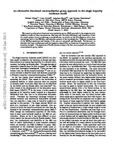
FIG. 1. Figure from Ref. 60 which compares new numerical values 共black circles兲 and a previous one 共white square兲 obtained for the exponent ␤ with our prediction from the FRG.

共1.19兲

which lies roughly at midpoint of the one-loop and two-loop prediction setting ⑀ ⫽1 in 共1.13兲. So do their most recent estimates59 for SR disorder. In d⫽2 this is ␨ ⫽0.753 ⫾0.002 and for d⫽3 they obtain 0.35⬍ ␨ ⬍0.4. These results 共1.16兲 and 共1.19兲 are close to estimates from the twoloop expansion and clearly rule out the NF conjecture. Another recent work60 studies an interface in the random field Ising model in high dimensions. The authors confirm that d⫽4 is the upper critical dimension. They further ex-

共1.20兲

The results are shown in Fig. 1. One can see a clear curvature downwards and that the straight line giving the 1-loop result is well above the obtained results 共the one-loop approximation would predict ␤ ⫽0.78 in d⫽2). Thus, although there is still some spread and uncertainty in the results, it seems that there is now a trend towards a convergence between theory and numerical simulations. The situation concerning experiments is presently unclear. Let us first outline the generic findings before analyzing the details. The measured exponents corresponding to LR elasticity and d⫽1 seem to be consistently in the range ␨ ⬇0.5 ⫺0.55. This is slightly above our two-loop result 共1.13兲 but not fully incompatible with it. Our calculation holds for quasistatic depinning, i.e., v ⬎0→0 ⫹ , and most experiments are also performed from the moving side, hopefully reaching the same quasistatic limit v →0 ⫹ . On the other hand if one believes that the numerical result 共1.19兲共also compatible with our calculation, from below兲 obtained for f ⫽ f ⫺ c also holds for quasistatic depinning 共a rather natural, but as yet unproved assumption兲 then one must conclude that the elastic models, in their simplest form at least, may not faithfully represent the experimental situation. Care must, however, be exercised before any such conclusion is reached. One could argue that disorder ⌬(u)⬃u ⫺ ␣ of range longer than RF ( ␣ ⬍1) could produce higher exponents ␨ ⫽ ⑀ /(2⫹ ␣ ) 共see end of Sec. IV A兲 but that does not seem to apply to those experiments where disorder is well controlled. Also, since the exponent ␨ ⫽0.5 is the Larkin DR exponent, which should hold below the Larkin length L c one must make sure that L c is well identified and that one is not simply observing a slow crossover to the asymptotic regime. In some of these experiments L c has been identified to be rather small. Let us now examine the situation in more detail.

174201-5


One much studied experimental system is the contact line of a fluid.12,61 It advances on a rough substrate and is pushed by adding fluid to the reservoir. The elasticity of the line is short range at short scale but at larger scales it is mediated by the elasticity of the two dimensional meniscus and thus it becomes long range and should be compared with Eqs. 共1.13兲, 共1.19兲. Disorder is random-field, but one should distinguish between microscopic disorder, which is poorly characterized, and macroscopic one which is well controlled. The situation has been studied for a helium meniscus on a macroscopically disordered substrate where ␨ ⫽0.55 was found.61 Although there are good indications that these experiments probe quasistatic depinning 共the contact line jumps from a reproducible pinned configuration to the next one兲 the precise nature of the dynamics remains open. Indeed it was found that propagation of perturbations along the line can be as fast as avalanches, showing inertial regime for helium.62 Experiments were repeated for viscous liquids63 yielding ␨ ⫽0.51⫾0.03. There it was checked that the system is overdamped and near depinning. In both cases there is also evidence of thermal activation effects13 characteristic of depinning 共not creep兲. It was argued that these may be a signature that a more complicated dynamics 共e.g., plastic兲 takes place at the very short scales and produces an effective dynamics at larger scales with complicated nonlinear 共e.g., exponential兲 velocity- and temperature-dependent damping. Very similar effects have also been shown to occur in solid friction64 where the activation volume was also found to correspond to microscopic scales. Another class of much studied experimental systems are crack fronts in heterogeneous media.65,66 These are characterized by two displacement fields, one out-of-plane component h and an in-plane one f. Cracks can either be studied stopped or slowly advancing. At the simplest level the inplane displacement f is expected to be described as an elastic line d⫽1, N⫽1 with LR elasticity c 兩 q 兩 , at quasistatic depinning.67 In experiments15,68 the observed roughness is again ␨ ⬇0.55. Since the crack propagates in an elastic medium, elastic waves which can in principle affect the roughness as the crack front advances producing a more complicated dynamics than Eq. 共1.3兲. Some proposals have been put forward on mechanisms to produce higher roughness exponents.69 They rely, however, on a finite velocity and it is unclear whether they can modify roughness in the quasistatic limit. Even if instantaneous velocities during avalanches become large enough, a detailed description on how these could change the line configurations remains to be understood. Then of course a major issue is whether the experiment, and in which sense, is in the quasistatic limit. There again microscopic dynamics could be more complex as at small scales the material may be damaged and the notion of a single front may not apply. Finally, since there are two components to displacement one should also be careful to understand interactions between them near depinning.70 Another interesting experimental system is a domain wall in a very thin magnetic film71 which experiences RB disorder. Up to now however only the thermally activated motion has been studied, which gives a quite remarkable confirmation of the creep law71 with RB exponents. It would be in-


teresting to study depinning there and to check whether it also belongs to the isotropic universality class. In that case, the crossover from RB to RF resulting in overhangs beyond some scale at zero temperature ( ␨ ⬎1) as well as the nontrivial thermal rounding of depinning could be studied. II. MODEL AND PERTURBATION THEORY

In this section we discuss some general features of the field theory of elastic manifolds in a random potential, both for the statics and for the dynamics, driven or at zero applied force. Some issues are indeed common to these three cases. At the end we specialize to depinning. A. Static and dynamical action and naive power counting

The static, equilibrium problem, can be studied using replicas. The replicated Hamiltonian corresponding to Eq. 共1.1兲 is H 1 ⫽ T 2T

冕兺

关共 ⵜu ax 兲 2 ⫹m 2 u ax 兴 ⫺

x a

1 2T 2

冕兺 x ab

R 共 u ax ⫺u bx 兲 , 共2.1兲

where, for now, we consider SR elasticity. a runs from 1 to n. We have added a small mass to provide an infrared cutoff, and we are interested in the large scale limit m→0. The limit of zero number of replicas n⫽0 is implicit everywhere. Terms with sums over three replicas or more corresponding to third or higher cumulants of disorder are generated in the perturbation expansion. These should in principle be included, but as we will see below higher disorder cumulants are not relevant for the T⫽0 depinning studied below. The dynamics, corresponding to the equation of motion 共1.3兲 is studied using the dynamical action averaged over disorder S关 uˆ ,u 兴 ⫽

冕

iuˆ xt 共 ␩ ⳵ t ⫺ ⳵ 2x ⫹m 2 兲 u xt ⫺ ␩ T

⫺

1 2

xt

冕

xtt ⬘

冕冕

iuˆ xt iuˆ xt ⬘ ⌬ 共 u xt ⫺u xt ⬘ 兲 ⫺

xt

iuˆ xt iuˆ xt

xt

iuˆ xt f xt . 共2.2兲

It generates disorder averaged correlations, e.g., 具 A 关 u xt 兴典 ⫽ 具 A 关 u xt 兴典 S with 具 A 典 S⫽ 兰 D关 u 兴 D关 uˆ 兴 Ae ⫺S and 具 1 典 S⫽1, and response functions ␦ 具 A 关 u 兴典 / ␦ f xt ⫽ 具 iuˆ xt A 关 u 兴典 S . The uniform driving force f xt ⫽ f ⬎0 共beyond threshold at T⫽0) may produce a velocity v ⫽ ⳵ t 具 u xt 典 ⬎0, a situation which we study by going to the comoving frame 共where 具 u xt 典 ⫽0) shifting u xt →u xt ⫹ v t, resulting in f → f ⫺ ␩ v . This is implied below. In general, for any value of f, we study the steady state, which at finite temperature T⬎0 is expected to be unique and time translational invariant 共TTI兲共all averages depend only on time differences兲. In the zero temperature limit, one needs a priori to distinguish the T⫽0 TTI theory as limL→⬁ limT→0 共e.g., the ground state in the static兲 and the T⫽0 ⫹ theory as limT→0 limL→⬁ .

174201-6



FIG. 2. 共i兲 Diagrammatic rules for the statics: replica propagator

具 u a u b 典 0 ⬅T ␦ ab /q 2 , unsplitted vertex, equivalent splitted vertex ⫺ 兺 ab (1/2T 2 )R(u a ⫺u b ) and 共ii兲 dynamics: response propagator 具 uˆ u 典 0 ⬅R q,t⫺t ⬘ , unsplitted vertex, splitted vertex uˆ xt uˆ xt ⬘ ⌬(u xt ⫺u xt ⬘ ) and temperature vertex. Arrows are along increasing time. An arbitrary number of lines can enter these functional vertices. 共iii兲 Unsplitted diagrams to one loop D, one loop with inserted one-loop counterterm G and two-loop A,B,C,E,F.

It is important to note that there are close connections, via the fluctuation dissipation relations, between the dynamical formalism and the statics. Indeed, at equilibrium 共for f ⫽0 and when time translation invariance is established兲 any equal time correlation function computed with Eq. 共2.2兲 is formally identical 共e.g., to all orders in perturbation theory兲 to the corresponding quantity computed in the equilibrium theory 共which is a single replica average兲. Similarly, the persistent parts, i.e., those ⬀ ␦ ( ␻ ), of dynamical correlations involving p mutually very separated times, are formally identical to the corresponding averages in the replica theory involving p replicas. The perturbative equilibrium calculations in the statics can thus be indifferently performed either with replicas or with Eq. 共2.2兲. It is possible to generate all dynamical graphs from static ones, a connection which, as will be further explained below, also carries to some extent to the case f ⬎0 at T⫽0. We first study ‘‘naive’’ perturbation theory and power counting. The quadratic part S 0 of the action 共2.2兲 yields the free response and correlation functions, used for perturbation theory in the disorder. They read

具 iuˆ q,t ⬘ u ⫺q,t 典 0 ⫽R q,t⫺t ⬘ ⫽

␪ 共 t⫺t ⬘ 兲 ⫺ (t⫺t ⬘ ) (q 2 ⫹m 2 ) ␩ e , ␩

具 u q,t ⬘ u ⫺q,t 典 0 ⫽C q,t⫺t ⬘ ,

共2.3兲

respectively, with the FDT relation TR q, ␶ ⫽⫺ ⳵ ␶ C q, ␶ ( ␶ ⬎0). Perturbation theory in ⌬(u) yields a disorder interaction vertex and at each 共unsplitted兲 vertex there is one conservation rule for momentum and two for frequency. It is thus convenient to use splitted vertices, as represented in Fig. 2, where the rules for the perturbation theory of the statics using replica are also given. For the dynamics one can also focus on T⫽0 where graphs are made only with response functions and consider temperature as an interaction vertex. The one-loop and two-loop diagrams which correct the dis-

order at T⫽0 are shown in Fig. 2 共unsplitted vertices兲. There are three types of two-loop graphs A,B,C. The graphs E and F lead to corrections proportional to temperature. At T⫽0 the model exhibits the property of dimensional reduction6,23–27 共DR兲 both in the statics and dynamics. Its ‘‘naive’’ perturbation theory, obtained by taking for the disorder correlator ⌬(u) an analytic function of u 关or R(u) for the statics兴, has a triviality property. As is easy to show using the above diagrammatic rules the perturbative expansion of any correlation function 具兿 i u x i t i 典 S in the derivatives ⌬ (n) (0) yields to all orders the same result as that obtained from the Gaussian theory setting ⌬(u)⬅⌬(0) 共the so called Larkin random force model兲. The same result holds for the statics, a for any correlation 具兿 i u x i 典 S . At T⫽0 these correlations are i

independent of the replica indices a i , their dynamical equivalent being independent of the times t i . The two point function thus reads to all orders:

具 u q,t ⬘ u ⫺q,t 典 DR⫽

⌬共 0 兲共 q ⫹m 2 兲 2 2

.

共2.4兲

This dimensional reduction results in a roughness exponent ␨ ⫽(4⫺d)/2 which is well known to be incorrect. One physical reason, in the statics, is that this amounts to solving the zero force equation which, whenever more than one solution exists, is not identical to finding the lowest energy configuration. Curing this problem, within a field theory, is highly nontrivial. One way to do that, as discussed later will be to consider a nonanalytic ⌬(u). It is important to note that despite the DR, dynamical averages involving response fields remain nontrivial, even at zero temperature. Perturbation theory at finite temperature also remains nontrivial. It is thus still useful to do power counting with an analytic ⌬(u), the modifications for a nonanalytic ⌬(u) being discussed in the following section. Power counting at the Gaussian fixed point yields t⬃x 2 and uˆ u⬃x ⫺d . At T⫽0 nothing else fixes the dimensions of u, since u→␭u, uˆ →␭ ⫺1 uˆ leaves the T⫽0 action invariant. Denoting u⬃x ␨ , ␨ is for now undetermined. The disorder term then scales as x 4⫺d⫹2 ␨ . It becomes relevant for d⬍4 provided ␨ ⬍(4⫺d)/2 which is physically expected 关for instance, in the random periodic case, ␨ ⫽0 is the only possible choice, and for other cases ␨ ⫽O( ⑀ )]. With this power counting the temperature term scales as x ⫺ ␪ with ␪ ⫽d⫺2⫹2 ␨ and is thus formally irrelevant near four dimension. In the end ␨ will be fixed by the disorder distribution at the fixed point.22 A more detailed study of divergences in the vertex functions allows to identify all counter-terms needed to render the theory finite. We denote by ˆ i ,q i , ␻ i 兲 ⌫ uˆ •••uˆ ;u•••u 共 qˆ i , ␻ Eu

⫽

E uˆ

␦

␦

兿兿 ˆˆ i⫽1 ␦ u q , ␻ j⫽1 ␦ u i

i

q j , ␻ˆ j

⌫ 关 u,uˆ 兴兩 u⫽uˆ ⫽0

共2.5兲

the irreducible vertex functions 共IVF’s兲 with E u external fields u 共at momenta q i , ␻ i , i⫽1, . . . ,E u ) and E uˆ external

174201-7



FIG. 3. Construction of diagrams starting from an unsplitted static diagram via two splitted static diagrams 共two-replica component兲 to the corresponding dynamical diagrams as explained in the text.

ˆ i , i⫽1, . . . ,E uˆ ). Being the derivafields 共at momenta qˆ i , ␻ tive of the effective action functional ⌫ 关 u,uˆ 兴 they are the important objects since all averages of products of u and uˆ fields are expressed as tree diagrams of the IVF. Finiteness of the IVF thus imply finiteness of all such averages. The present theory has the property of covariance under the well known statistical tilt symmetry STS u xt →u xt ⫹g x , which yields that the two point vertex ⌫ uˆ u ( ␻ ⫽0) remains uncorrected to all orders. This allows to fix the elastic constant c ⫽1 and shows that the mass term is uncorrected and can thus safely be used as an IR cutoff. It also implies that all higher IVF’s vanish when any of the ␻ i is set to zero. The DR result is a perturbative triviality statement about ˆ i ) at T⫽0, all other cases remain nontrivial. In a ⌫ uˆ •••uˆ (qˆ i , ␻ sense we will now expand around dimensional reduction. Similar replica IVF’s can be defined for the statics. Perturbation expansion of a given IVF to any given order in the disorder can be represented by a set of one particle irreducible 共1PI兲 graphs. As mentionned above there is a simple rule to generate the dynamical graphs from the static ones. The static propagator being diagonal in replicas, each static graph occurring in a p replica IVF contains p connected components. At T⫽0 the rule is then to attach one response field to each connected component of the static diagram, each replica graph then generating one or more dynamical graphs. The place where the response field is attached is the root of the diagram. The direction of the remaining response functions is then fixed unambiguously, always pointing towards the root. This procedure to deduce the dynamical diagrams from the static ones is unique and exhaustive and is illustrated in Fig. 3. A generalization exists at T⬎0 but is not needed here. Any graph corresponding to a given dynamical IVF contains p connected components 共in the splitted diagrammatics兲 with 1⭐ p⭐E uˆ (p⫽E uˆ at T⫽0), each one leading to a conservation rule between external frequencies, and thus one can write symbolically: ˆ i ,q i , ␻ i 兲 ⌫ uˆ •••uˆ ;u•••u 共 qˆ i , ␻ ⫽␦

冉兺

qˆ ⫺

兺

冊兿冉兺 p

q

i⫽1

␦

␻ˆ ⫺

兺␻

冊

˜⌫ . 共2.6兲

Let us compute the superficial degree of UV divergence ␣ of such a graph with v ⌬ disorder vertices and v T temperature factors contributing to ˜⌫ ⬃⌳ ␣ . Using momentum and frequency conservation laws at each vertex, and since there are only response functions E uˆ ⫹I⫽2( v ⌬ ⫹ v T ) we obtain

␣ ⫽d⫹2 p⫺dE uˆ ⫹ 共 d⫺4 兲v ⌬ ⫹ 共 d⫺2 兲v T .

共2.7兲

At T⫽0 ( v T ⫽0,p⫽E uˆ ) at the critical dimension d⫽4 the only superficially UV divergent IVF are those with one external uˆ 共quadratic divergence兲 or two external uˆ 共logarithmic divergence LD兲. The STS further restricts the possible divergent diagrams. One sees that only three types of counter-term are needed a priori. One counterterms is needed for the ⌳ 2 divergence of ⌫ uˆ (q⫽0,␻ ⫽0) 共excess force f ⫺ ␩ v in driven dynamics兲. This is analogous to the mass in the ␾ 4 theory, i.e., the distance to criticality. If we are exactly at the depinning critical point ( f ⫽ f c ) we need not worry about this divergence. Another counterterm is associated with the LD in ␩ and the last one with the LD in the second cumulant of disorder ⌬(u), i.e., a full function, which makes it different from the conventional FT for critical phenomena 共e.g., ␾ 4 ). One notes that higher cumulants are formally irrelevant, as they involve E uˆ ⬎2. One sees from Eq. 共2.7兲 that each insertion of a temperature vertex yields an additional quadratic divergence in d ⫽4, more generally a factor T⌳ d⫺2 . Thus to obtain a theory where observables are finite as ⌳→⬁ one must start from a model where the initial temperature scales with the UV cutoff as ˜ m ⫺␪ T⫽T

冉冊 m ⌳

d⫺2

.

共2.8兲

This is similar to the ␾ 4 theory where it is known that a ␾ 6 term can be present and yields a finite UV limit 共i.e., does not spoil renormalizability兲 only if it has the form g 6 ␾ 6 /⌳ d⫺2 . It then produces only a finite shift to g 4 without changing universal properties.72 Here each ˜T factor will thus come with a ⌳ 2⫺d factor which compensates the UV divergence. Computing the resulting shift in ⌬(u) to order ⌬ 2 by resumming the diagrams E and F of Fig. 2 and all similar diagrams to any number of loops has not been attempted here.

174201-8



For convenience we have inserted factors of m in the definition of the rescaled temperature, using the freedom to rescale u by m ⫺ ␨ and uˆ by m ␨ . The disorder term then reads as ˜ (um ␨ ) in in Eq. 共2.2兲 with ⌬(u) replaced by ⌬ 0 (u)⫽m ⑀ ⫺2 ␨ ⌬ ˜. terms of a dimensionless rescaled function ⌬ B. Nonanalytic field theory and depinning in the quasistatic limit

From now on we study the zero temperature limit T⫽0. To escape the DR triviality phenomenon, and since the fixed points found in one-loop studies exhibit a cusp at u⫽0, we must consider perturbation theory in a nonanalytic disorder correlator. In this section we show how to develop perturbation theory and diagrammatics in a nonanalytic theory and what are the nontrivial issues which arise. For now the considerations apply for zero or finite applied force. In usual diagrammatics, extracting a leg from a vertex corresponds to a derivation. Here this can be done as usual with no ambiguity, provided the corresponding vertex is evaluated at a generic u 共e.g., the graphs in Fig. 3兲. If the vertex is evaluated at u⫽0 共here and in the following we call them saturated vertices兲 one must go back to a careful application of Wick’s rules. Any graph containing such a vertex and which vanishes in the analytic theory is called anomalous. Let us write the series expansion in powers of 兩 u 兩 : 1 ⌬ 共 u 兲 ⫽⌬ 共 0 兲 ⫹⌬ ⬘ 共 0 ⫹ 兲兩 u 兩 ⫹ ⌬ ⬙ 共 0 ⫹ 兲 u 2 ⫹••• . 共2.9兲 2 Wick’s rules can then be applied but usually end up in evaluating nontrivial averages of, e.g., sign or delta functions. Let us consider as an example the following two-loop 1PI diagram 共noted e 1 in what follows兲 which is a correction to the effective action of the form:

共2.10兲 Here four Wick contractions have been performed, as in any of the other thirty two-loop diagrams of the form A 共studied in the next section兲. In an analytic theory performing the local time expansion this would result in a two-loop correction to ⌬(u) proportional to ⌬ ⬙ (u) but with a zero coefficient since the ⌬ ⬘ functions are evaluated at zero argument. In the nonanalytic theory, inserting the expansion 共2.9兲 yields 共upon some change of variables兲 e 1 ⫽⌬ ⬘ 共 0 ⫹ 兲 2 ⌬ ⬙ 共 u 兲

冕

t i ⬎0,r i

R r 1 ,t 1 R r 1 ,t 2 R r 3 ⫺r 1 ,t 3 R r 3 ,t 4 F r i ,t i ,

F r i ,t i ⫽ 具 sgn共 X 兲 sgn共 Y 兲典 ,

共2.11兲

X⫽u r 1 ,⫺t 3 ⫺u r 1 ,⫺t 4 ⫺t 1 , Y ⫽u 0,⫺t 4 ⫺u 0,⫺t 3 ⫺t 2 terms of higher order in Eq. 共2.9兲 do not contribute since we are at T⫽0 and we have exhausted the number of uˆ to contract 共i.e., those terms would yield higher orders in T). The remaining average in Eq. 共2.11兲 is evaluated with respect to a Gaussian measure, and can thus be performed. It can be defined by using the T⬎0, v ⬎0 Gaussian measure (u xt → v t ⫹u xt ) and taking the limit T→0, v →0. The result is a continuous function of v 2 /T and its value depends on how the limit is taken. In the static theory one should take T→0 at v ⫽0. This yields 2 ␲

具 sgn共 X 兲 sgn共 Y 兲典 ⫽ asin共 ␴ 兲 ␴⫽

具 XY 典

冑具 X 2 典冑具 Y 2 典

共2.12兲

,

i.e., the result for centered Gaussian variables. Expressing the averages in Eq. 共2.12兲 using correlation functions C q,t yields a complicated T⫽0 expression for e 1 . This expression will be discussed in a companion paper on the statics.34 A list of all anomalous diagrams is presented in Appendix K. The opposite limit v →0 at T⫽0 yields much simpler expressions:

具 sgn共 X 兲 sgn共 Y 兲典 →sgn共 t 4 ⫹t 1 ⫺t 3 兲 sgn共 t 3 ⫹t 2 ⫺t 4 兲 . More generally this procedure corresponds to the substitution ⌬ (n) (u r,t ⫺u r,t ⬘ )→⌬ (n) 关v (t⫺t ⬘ ) 兴 in any ambiguous vertex evaluated at u⫽0. That this is the correct definition of the theory of the quasistatic depinning as the limit v ⫽0 ⫹ is particularly clear here since it is well known 共the no passing property9,44兲 that the u r,t are increasing functions of time in the steady state. Of course it remains to be shown that the procedure actually works and does not produce singular terms such as ␦ ( v t). It also remains to be shown that it yields a renormalizable continuum theory where all divergences can be removed by the appropriate counterterms. This is far from trivial and will be achieved below. Let us comment again on the connections between dynamics and statics. Consider a T⫽0 dynamical diagram with p connected components evaluated at zero external frequencies. All response functions can be integrated over the times from the leaves towards the root on each connected component. Using the FDT relation this replaces response by correlations and thus exactly reproduces a p replica static diagram except that it is differentiated once with respect to each replica field 共the sums over all possible positions of the response field reproduces the derivation chain rule兲. One simple way to establish this rule is to consider the formal limit ␩ →0 ⫹ 共equivalently expansion of R q, ␻ in powers of frequency兲, i.e., formally replace R q,t,t ⬘ → ␦ tt ⬘ /q 2 共keeping track of causality兲. This reproduces exactly the zero frequencies dynamical diagrams and treats ‘‘replicas’’ as ‘‘times.’’

174201-9


Thus the pth derivative of a p replica static diagram gives a set of dynamical diagrams with p connected components. For p⫽2 this ensures, e.g., that the relation ⌬(u)⫽ ⫺R ⬙ (u) remains uncorrected to all orders. The flaw in this argument comes from the anomalous diagrams 共both in statics and dynamics兲. In the analytic theory the dynamical diagrams with response fields on a saturated vertex vanish or cancel in pairs. This just expresses that taking a derivative of a static saturated vertex gives zero and the rule still works. But in the nonanalytic theory the anomalous diagrams do not vanish and contain an additional time dependence. The above integration of response functions from the leaves to the root cannot be performed for these anomalous diagrams. As a result they can give nontrivial contributions both in statics and dynamics which violate relations such as ⌬(u) ⫽⫺R ⬙ (u), thus allowing us to distinguish statics from depinning. To conclude this section: The perturbative calculation of the effective action and of the IVF vertices can also be performed in a nonanalytic theory. It can be expressed as sums of the same diagrams one writes in the analytic theory, with the same graphical rules to draw and generate the diagrams starting from the statics. However the way to compute these diagrams and their values is different from the analytic theory. The time ordering of vertices comes in a non-trivial way and produces results which can be different at depinning ⫹ f⫽f⫹ c ( v ⫽0 ) and in the statics f ⫽0, as illustrated on the diagram e 1 above. Thus we see the principle mechanism by which the statics and the depinning can yield different field theories, which is a novel result. It remains to perform the actual calculation of these nonanalytic diagrams, which is performed in the following sections. III. RENORMALIZATION PROGRAM

In this section we will compute the effective action to two-loop order at T⫽0 for depinning. From the above analysis we know that we only need to compute the one- and two-loop corrections to ⌬(u) and ␩ . A. Corrections to disorder

We start by the corrections to the disorder, first at oneloop and then at two-loop order.

FIG. 4. One-loop dynamical diagrams correcting ⌬.


FIG. 5. The three possible classes at second order correcting disorder at T⫽0. Only classes A and B will contribute. 1. One loop

At leading order, there are four diagrams, depicted in Fig. 4. Since diagram 共d兲 is proportional to ⌬ ⬘ (u)⌬ ⬘ (0), it is an odd function of u, and thus does not contribute to the renormalization of ⌬. However its repeated counterterm will appear at two-loop order. Diagram 共a兲 is proportional to ⫺⌬(u)⌬ ⬙ (u), diagram 共b兲 to ⫺⌬ ⬘ (u) 2 and diagram 共c兲 to ⌬ ⬙ (u)⌬(0). All come with a combinatorial factor of 1/2! from Taylor-expanding the exponential function, 1/2 from the action and 4 from combinatorics. Together, they add up to the one-loop correction to disorder

␦ 1⌬共 u 兲⫽

4 兵 ⫺⌬ ⬘ 共 u 兲 2 ⫺ 关 ⌬ 共 u 兲 ⫺⌬ 共 0 兲兴 ⌬ ⬙ 共 u 兲其 I 1 , 2!2 I 1ª

冕

q

1 共 q ⫹m 2 兲 2 2

,

共3.1兲

2

with I 1 ⫽ 兰 q e ⫺q ⌫(2⫺d/2)m ⫺ ⑀ ⫽(4 ␲ ) ⫺d/2⌫(2⫺d/2)m ⫺ ⑀ . 2. Two loops

First, we have to find all diagrams correcting disorder at second order. At T⫽0 they can be grouped in three classes A, B, and C for the three possible diagrams for unsplitted vertices. Class C does not contribute as is shown in Appendix C. We begin our analysis with class A. We now need to write all possible diagrams with splitted vertices of type A. A systematic procedure is to start from all possible static diagrams given in Fig. 6. This relies on the fact that dynamics and statics are related—recall that in general a dynamic formulation can be used to obtain the renormalization of the statics. As mentioned in the previous section, to go from the statics to the dynamics, one attaches one response field to a root on each connected component of the diagrams a to f in Fig. 6 and orient each component towards

FIG. 6. Static graphs at 2-loop order in the form of a hat 共class A in Fig. 5兲 contributing to two replica terms. Adding a responsefield to each connected component leads to the dynamic diagrams of Fig. 7. 174201-10



FIG. 7. Dynamical diagrams at two-loop order of type A with two external response fields 共two connected components兲 correcting the disorder; derived from the two replica static diagrams of Fig. 6.

the root. The result is presented in Fig. 7. The next step is to eliminate all diagrams which yield odd functions of u and thus do not contribute to the renormalized disorder. The list is the following:

␦ 2⌬共 u 兲⫽ ⫽

a 1 ⫽a 4 ⫽c 3 ⫽d 1 ⫽d 3 ⫽d 5 ⫽d 7 ⫽e 2 ⫽e 3 ⫽ f 1 ⫽ f 3 ⫽ f 4 ⫽ f 5 ⫽0.

共3.2兲

Further simplifications come from diagrams, which mutually cancel. Again this uses that ⌬ ⬘ (u) is an odd function. This gives c 2 ⫹c 5 ⫽d 2 ⫹d 4 ⫽d 6 ⫹d 8 ⫽0.

共3.3兲

c 4 ⫽0,

共3.4兲

In addition

since 兰 tt ⬘ R xt R xt ⬘ ⌬ ⬘ (t⫺t ⬘ )⫽0. This is explained in more details in Appendix K where the list of all anomalous 共nonodd兲 graphs is given together with their expressions in the nonanalytic field theory. Thus, the only nonzero graphs which we have to calculate are a 2 ,a 3 ,b 1 , . . . ,b 6 , c 1 , e 1 , and f 2 . These calculations are rather cumbersome, due to the appearance of theta functions of sums or differences of times as a result of the nonanalyticity of the theory. The correction to disorder is

1 2 3共 23兲 3! 2 3

兺共 a i ⫹b i ⫹••• 兲

兺共 a i ⫹b i ⫹••• 兲 ,

where the combinatorial factors are 1/3! from the Taylor expansion of the exponential function, 2/23 from the explicit factors of 1/2 in the interaction, a factor of 3 to choose the vertex at the top of the hat, and a factor of 2 for the possible two choices in each of the vertices. Furthermore below some additional combinatorial factors are given: a factor of 2 for generic graphs and 1 if it has the mirror symmetry with respect to the vertical axis: each diagram symbol (a i •••) denotes the diagram including the symmetry factor. We recall that we have defined saturated vertices as vertices evaluated at u⫽0 while unsaturated vertices still contain u explicitly. Diagrams with response functions added to unsaturated vertices can be obtained by deriving static diagrams a 2 ⫹a 3 ⫽second derivative of the statics, b 1 ⫹b 2 ⫹b 3 ⫹b 4 ⫹b 5 ⫹b 6 ⫽second derivative of the statics.

共3.5兲

The graphs which contain external response fields on saturated vertices cannot be derivatives from static ones. For class A, the hat diagrams, the only nonzero such graph is c 1 . Explicitly, this reads

174201-11



FIG. 8. Two-loop dynamical diagrams of type B 共see Fig. 5兲.

a 2 ⫹a 3 ⫽⫺ ⳵ 2u 关 ⫺R ⬙ 共 0 兲 R ⵮ 共 u 兲 2 兴 I A ,

共3.6兲

where 关see Eq. 共A18兲兴 I Aª

冕

冉

d dq 1 d dq 2

1

1

1

共2␲兲共2␲兲

q 21 ⫹m 2

q 22 ⫹m 2

关共 q 1 ⫹q 2 兲 ⫹m 兴

d

d

2

⫽

2 2

冊

1

I lª

共3.7兲

共 q 21 ⫹m 2 兲共 q 22 ⫹m 2 兲共 q 23 ⫹m 2 兲共 q 21 ⫹q 23 ⫹2m 2 兲

ln 2 共 ⑀ I 1 兲 2 ⫹finite. 2⑀

⫻e ⫺{ 关 (q 1 ⫹q 2 )

6

兺 b i ⫽⫺ ⳵ 2u 关 R ⬙共 u 兲 R ⵮共 u 兲 2 兴 I A

and c 1 ⫽2⌬ ⬘ 共 0 ⫹ 兲 2 ⌬ ⬙ 共 u 兲 I A .

共3.9兲

The diagram e 1 is an explicit example for the appearance of nontrivial sign functions resulting from the monotonic increase of the displacement. It was already discussed in the previous section. In the quasistatic depinning limit 共2.11兲 gives 共details are given in Appendix A兲:

冕冕 q 1 ,q 2

共3.12兲

t 1 ,t 2 ,t 3 ,t 4 ⬎0

sgn共 t 4 ⫺t 3 ⫺t 2 兲

2 ⫹m 2 ](t ⫹t )⫹(q 2 ⫹m 2 )t ⫹(q 2 ⫹m 2 )t } 3 4 1 2 1 2

共3.13兲

In Appendix A we show that 共for any given elasticity兲 the sum of e 1 ⫹ f 2 only involves the integral I A , and that the combination takes the simpler form e 1 ⫹ f 2 ⫽⫺⌬ ⬘ 共 0 ⫹ 兲 2 ⌬ ⬙ 共 u 兲 I A .

共3.14兲

We now turn to graphs of type B 共bubble diagrams, see Fig. 8兲. Again diagrams, which are odd functions of u vanish. These are 共3.15兲

Two other diagram mutually cancel:

2 )t ⫹(q 2 ⫹m 2 )t ⫹[(q ⫹q ) 2 ⫹m 2 ](t ⫹t ) 1 2 1 2 3 4 其 2

共3.10兲

The result of the explicit integration is e 1 ⫽⌬ ⬘ 共 0 ⫹ 兲 2 ⌬ ⬙ 共 u 兲关 I l ⫺I A ⫹finite兴 ,

q 1 ,q 2

h 1 ⫽h 2 ⫽i 1 ⫽ j 1 ⫽k 2 ⫽k 3 ⫽l 2 ⫽l 3 ⫽l 4 ⫽0.

t 1 ,t 2 ,t 3 ,t 4 ⬎0

⫻sgn共 t 1 ⫺t 3 ⫹t 4 兲 sgn共 t 2 ⫺t 4 ⫹t 3 兲 .

冕冕

⫽⫺⌬ ⬘ 共 0 ⫹ 兲 2 ⌬ ⬙ 共 u 兲 I l .

共3.8兲

i⫽1

2

q 1 ,q 2

f 2 ⫽2⌬ ⬘ 共 0 ⫹ 兲 2 ⌬ ⬙ 共 u 兲

Furthermore, we find

⫻e ⫺ 兵 (q 1 ⫹m

1

The last diagram f 2 also involves a sign function and reads

1 ⫽ ⫹ ⫹O 共 ⑀ 2 兲共 ⑀ I 1 兲 2 . 2 4 ⑀ 2⑀

e 1 ⫽⌬ ⬘ 共 0 ⫹ 兲 2 ⌬ ⬙ 共 u 兲

冕

共3.11兲

k 1 ⫹l 1 ⫽0,

共3.16兲

as discussed in Appendix K. The diagrams that are second derivative of the static have all their response fields on their unsaturated vertices. These are

174201-12



g 1 ⫹g 2 ⫹g 3 ⫹g 4 ⫽ ⳵ 2u

冋

册

1 ⌬ 共 u 兲 2 ⌬ ⬙ 共 u 兲 I 21 , 2

h 3 ⫹h 4 ⫹h 5 ⫹h 6 ⫽ ⳵ 2u 关 ⫺⌬ 共 0 兲 ⌬ 共 u 兲 ⌬ ⬙ 共 u 兲兴 I 21 , i 2 ⫽ j 2 ⫽ ⳵ 2u

冋

FIG. 9. One-loop dynamical diagram correcting the friction.

册

function, we can expand (u xt ⫺u xt ⬘ ) in a Taylor-series, of which only the first term contributes. Equation 共3.22兲 becomes

1 ⌬ 共 0 兲 2 ⌬ ⬙ 共 u 兲 I 21 . 4

冕

The surprise is that i 3 , which is not the second derivative of a static diagram, since it has both response fields on saturated vertices, is nontrivial: ⫹ 2

i 3 ⫽⫺⌬ ⬘ 共 0 兲

⌬ ⬙ 共 u 兲 I 21 .

共3.17兲

To summarize, for the driven problem at T⫽0 in perturbation of ⌬⬅⌬(u), the contributions to the disorder to one and two loops, i.e., the corresponding terms in the effective action ⌫ 关 u,uˆ 兴 are

␦ 1 ⌬ 共 u 兲 ⫽⫺ 兵 ⌬ ⬘ 共 u 兲 2 ⫹ 关 ⌬ 共 u 兲 ⫺⌬ 共 0 兲兴 ⌬ ⬙ 共 u 兲其 I 1

共3.18兲

t⬎t ⬘ ,x

冕

␦␩ ⫽⫺⌬ ⬙ 共 0 ⫹ 兲 tR r⫽0,t .

Here, the response function is taken at spatial argument 0. In momentum representation, the same expression reads

␦␩ ⫽⫺⌬ ⬙ 共 0 ⫹ 兲

共3.19兲

Curiously, even though two diagrams contain contributions proportional to I l ⬃ln 2, these contributions cancel in the final result for the corrections to the disorder.

⫽⫺⌬ ⬙ 共 0 ⫹ 兲

冕

t⬎t ⬘ ,x

iuˆ xt ⌬ 共 u xt ⫺u xt ⬘ 兲 iuˆ xt ⬘ .

共3.20兲

t⬎t ⬘ ,x

iuˆ xt ⌬ ⬘ 共 u xt ⫺u xt ⬘ 兲 R r⫽0,t⫺t ⬘ .

tR q,t ⫽⫺⌬ ⬙ 共 0 ⫹ 兲

t

q

q

共 q ⫹m 2 兲 2

1 2

冕冕 t

te ⫺t(q

2 ⫹m 2 )

q

⫽⫺⌬ ⬙ 共 0 ⫹ 兲 I 1

1 8

␦␩ ⫽⫺ ⫻4⫻2 关 a⫹b⫹c⫹d⫹e⫹ f ⫹g 兴 .

共3.25兲

共3.26兲

The combinatorial factor is 1/8 from the interaction, 4 from the time ordering of the vertices, and an additional factor of 2 for the symmetry of diagrams a, b, e, f, and g. Details of the calculation of diagrams a to g are given in Appendix D. Grouping diagrams, which partially cancel, we find a⫹g⫽⫺⌬ ⬙ 共 0 ⫹ 兲 2 I 21 ,

Contracting one iuˆ xt ⬘ leads to

冕

冕冕冕

with the already known integral I 1 , Eq. 共3.1兲. We now turn to the two-loop corrections. There are seven contributions, drawn on Fig. 10. Their contribution to ␩ is

B. Corrections to the friction ␩

We now calculate the divergent corrections to ␩ , which will require a counterterm proportional to iuˆ u˙ . Let us illustrate their calculation at leading order. We start from the first order expansion of the interaction e ⫺S int, which can be written as

共3.24兲

t

2

⫻⌬ ⬙ 共 u 兲其 ⬙ I 21 ⫹⌬ ⬘ 共 0 ⫹ 兲 2 ⌬ ⬙ 共 u 兲共 I A ⫺I 21 兲 .

共3.23兲

The correction to friction at leading order thus is 共see Fig. 9兲

1 ␦ ⌬ 共 u 兲 ⫽ 兵关 ⌬ 共 u 兲 ⫺⌬ 共 0 兲兴 ⌬ ⬘ 共 u 兲其 ⬙ I A ⫹ 兵关 ⌬ 共 u 兲 ⫺⌬ 共 0 兲兴 2 2 2

iuˆ xt 关共 t⫺t ⬘ 兲 u˙ xt ⫹O 共 t⫺t ⬘ 兲 2 兴 ⌬ ⬙ 共 0 ⫹ 兲 R r⫽0,t⫺t ⬘ .

共3.27兲

共3.21兲

The response function contains a short-time divergence, which we deal with in an operator product expansion. Expanding ⌬ ⬘ (u xt ⫺u xt ⬘ ) to the necessary order yields

冕

t⬎t ⬘ ,x

iuˆ xt 关 ⌬ ⬘ 共 0 ⫹ 兲 ⫹ 共 u xt ⫺u xt ⬘ 兲 ⌬ ⬙ 共 0 ⫹ 兲 ⫹••• 兴 R r⫽0,t⫺t ⬘ . 共3.22兲

The first term of this expansion, proportional to ⌬ ⬘ (0 ⫹ ), is strongly UV divergent and nonuniversal and gives the critical force to lowest order in disorder. Since we tune f to be exactly at the depinning threshold we do not need to consider it. The second contribution, proportional to ⌬ ⬙ (0 ⫹ ), corrects the friction: due to the short-range singularity in the response

FIG. 10. Two-loop dynamical diagrams correcting the friction. They all have multiplicity 8 except c and d which have multiplicity 4.

174201-13



1 b⫹c⫹d⫽⫺ ⌬ ⵮ 共 0 ⫹ 兲 ⌬ ⬘ 共 0 ⫹ 兲 I 21 , 2

共3.28兲

The ␤ function is by definition the derivative of ⌬ at fixed ⌬ 0 . It reads

e⫽⫺⌬ ⵮ 共 0 ⫹ 兲 ⌬ ⬘ 共 0 ⫹ 兲 I ␩ ,

共3.29兲

⫺m ⳵ m ⌬ 兩 ⌬ 0 ⫽ ⑀ 关 m ⫺ ⑀ ⌬ 0 ⫹2 ␦ (1) 共 m ⫺ ⑀ ⌬ 0 兲 ⫹3 ␦ (2) 共 m ⫺ ⑀ ⌬ 0 兲

f ⫽⫺2⌬ ⵮ 共 0 ⫹ 兲 ⌬ ⬘ 共 0 ⫹ 兲 I A ⫺2⌬ ⬙ 共 0 ⫹ 兲 2 I A .

共3.30兲

This involves the nontrivial diagram I ␩ I ␩ª

⫽

冕

冉

1 2⑀

2

共 q 21 ⫹m 2 兲共 q 22 ⫹m 2 兲 2 共 q 22 ⫹q 23 ⫹2m 2 兲

⫹

冊

1⫺2 ln 2 共 ⑀ I 1 兲 2 ⫹finite 4⑀

Using the inversion formula 共3.35兲, the ␤ function can be written in terms of the renormalized disorder ⌬:

共3.31兲

In order to proceed, let us calculate the repeated one-loop counterterm ␦ 1,1(⌬). We start from the one-loop counterterm 共3.18兲, which has the bilinear form 1 2

␦ (1) 共 f ,g 兲 ⫽⫺ 兵 2 f ⬘ 共 u 兲 g ⬘ 共 u 兲 ⫹ 关 f 共 u 兲 ⫺ f 共 0 兲兴 g ⬙ 共 u 兲

calculated in Appendix E. C. Renormalization program to two loops and calculation of counter-terms 1. Renormalization of disorder

Let us now discuss the strategy to renormalize the present theory where the interaction is not a single coupling constant, but a whole function, the disorder correlator ⌬(u). We denote by ⌬ 0 the bare disorder—this is the object in which perturbation theory is carried out—i.e., one consider the bare action 共2.2兲 with ⌬→⌬ 0 . We denote here by ⌬ the renormalized dimensionless disorder i.e. the corresponding term in the effective action ⌫ 关 u,uˆ 兴 is m ⑀ ⌬. We define the dimensionless bilinear one-loop and trilinear two-loop symmetric functions 关see Eqs. 共3.18兲 and 共3.19兲兴 such that

␦ (1) 共 ⌬,⌬ 兲 ⫽m ⑀ ␦ 1 ⌬,

共3.32兲

␦ (2) 共 ⌬,⌬,⌬ 兲 ⫽m 2 ⑀ ␦ 2 ⌬

共3.33兲

⫹ 关 g 共 u 兲 ⫺g 共 0 兲兴 f ⬙ 共 u 兲其˜I 1

⌬⫽m

⌬ 0⫹ ␦

(1)

共m

⫺⑀

⌬0兲⫹␦

(2)

共m

⫺⑀

⌬ 0 兲 ⫹O 共 ⌬ 40 兲 .

共3.34兲

It contains terms of order 1/⑀ and 1/⑀ 2 . This is sufficient to calculate the RG functions at this order. 共In principle, one has to keep the finite part of the one-loop terms, but we will work in a scheme, where these terms are exactly 0, by normalizing all diagrams by the one-loop diagram兲. Inverting this formula yields ⌬ 0 ⫽m ⑀ 关 ⌬⫺ ␦ (1) 共 ⌬ 兲 ⫺ ␦ (2) 共 ⌬ 兲 ⫹ ␦ (1,1) 共 ⌬ 兲 ⫹••• 兴 , 共3.35兲 where ␦ (1,1) (⌬) is the one-loop repeated counterterm

␦ (1,1) 共 ⌬ 兲 ⫽2 ␦ (1) 关 ⌬, ␦ (1) 共 ⌬,⌬ 兲兴 .

共3.36兲

共3.39兲

with the dimensionless integral ˜I 1 ªI 1 兩 m⫽1 ; we will use the same convention for ˜I A ªI A 兩 m⫽1 . Thus ␦ 1,1(⌬) reads

␦ (1,1) 关 ⌬ 共 u 兲兴 ⫽2 ␦ (1) 关 ⌬, ␦ (1) 共 ⌬ 兲兴 ⫽ 兵关 ⌬ 共 u 兲 ⫺⌬ 共 0 兲兴 2 ⌬ ⬙ 共 u 兲 ⫹ 关 ⌬ ⬘ 共 u 兲 2 ⫺⌬ ⬘ 共 0 兲 2 兴关 ⌬ 共 u 兲 ⫺⌬ 共 0 兲兴其 ⬙˜I 21 . 共3.40兲 Note that this counterterm is nonambiguous for u→0. Finally, as discussed at the end of the previous section at any point we can rescale the fields u by m ␨ . This amounts to ˜ (um ␨ ) write the ␤ function for the function ⌬(u)⫽m ⫺2 ␨ ⌬ which will be implicit in the following 共in addition we will drop the tilde superscript兲. The two-loop ␤ function 共3.38兲 then becomes with the help of Eq. 共3.40兲 ⫺m ⳵ m ⌬ 共 u 兲 ⫽ 共 ⑀ ⫺2 ␨ 兲 ⌬ 共 u 兲 ⫹ ␨ u⌬ ⬘ 共 u 兲

thus extended to nonequal argument using f (x,y)ª 21 关 f (x ⫹y,x⫹y)⫺ f (x,x)⫺ f (y,y) 兴 and a similar expression for the trilinear function. Whenever possible we will use the shorthand notation ␦ (1) (⌬)⫽ ␦ (1) (⌬,⌬) and ␦ (2) (⌬) ⫽ ␦ (2) (⌬,⌬,⌬). The expression of ⌬ obtained perturbatively in powers of ⌬ 0 at two-loop order reads ⫺⑀

共3.37兲

⫺m ⳵ m ⌬ 兩 ⌬ 0 ⫽ ⑀ 关 ⌬⫹ ␦ (1) 共 ⌬ 兲 ⫹2 ␦ (2) 共 ⌬ 兲 ⫺ ␦ (1,1) 共 ⌬ 兲 ⫹••• 兴 . 共3.38兲

1

q 1 ,q 2

⫹••• 兴 .

1 ⫺ 兵关 ⌬ 共 u 兲 ⫺⌬ 共 0 兲兴 2 其 ⬙ 共 ⑀˜I 1 兲 2 ⫹ 兵关 ⌬ 共 u 兲 ⫺⌬ 共 0 兲兴 ⌬ ⬘ 共 u 兲 2 其 ⬙ ⑀ 共 2˜I A ⫺˜I 21 兲 ⫹⌬ ⬘ 共 0 ⫹ 兲 2 ⌬ ⬙ 共 u 兲 ⑀ 共 2˜I A ⫺˜I 21 兲 .

共3.41兲

One of our main results is now apparent: the 1/⑀ terms cancel in the corrections to disorder. If it had not been the case it would lead to a term of order 1/⑀ in the ␤ function and thus to nonrenormalizability. Thus the ␤ function is finite to two loops a hallmark of a renormalizable theory. Note that this happened in a rather nontrivial way since it required a consistent evaluation of all anomalous nonanalytic diagrams. Furthermore the precise type of cancellation is unusual: usually the two-loop bubble diagrams of type B are simply the square of the one-loop ones. Here the easily missed and nontrivial bubble diagram i 3 was crucial in achieving the above cancellation. In order to simplify notations and further calculations, we absorb a factor of ⑀˜I 1 in the definition of the renormalized

174201-14

2



disorder 共or equivalently in the normalization of momentum or space integrals兲. With this, the ␤ function takes the simple form

and thus 共remind that I 1 ⬃m ⫺ ⑀ and I A ⬃I ␩ ⬃m ⫺2 ⑀ ) m

⫺m ⳵ m ⌬ 共 u 兲 ⫽ 共 ⑀ ⫺2 ␨ 兲 ⌬ 共 u 兲 ⫹ ␨ u⌬ ⬘ 共 u 兲

d ln Z ⫺1 ⫽⌬ 0⬙ 共 0 ⫹ 兲共 ⑀ I 1 兲 ⫺⌬ 0⬙ 共 0 ⫹ 兲 2 ⑀ 共 I 21 ⫹4I A 兲 dm 2 ⫹ ⫹ ⫹⌬ ⵮ 0 共 0 兲⌬⬘ 0 共 0 兲 ⑀ 共 I 1 ⫹4I A ⫹2I ␩ 兲 .

1 ⫺ 兵关 ⌬ 共 u 兲 ⫺⌬ 共 0 兲兴 2 其 ⬙ 2

共3.47兲

1 ⫹ 兵关 ⌬ 共 u 兲 ⫺⌬ 共 0 兲兴 ⌬ ⬘ 共 u 兲 2 其 ⬙ 2 1 ⫹ ⌬ ⬘共 0 ⫹ 兲 2⌬ ⬙共 u 兲 . 2

共3.42兲

Note several interesting features of this two-loop ␤ function. First it contains a nontrivial so called ‘‘anomalous term’’ 共the last one兲 which is absent in an analytic theory. Second, it can be shown to exhibit irreversibility, precisely due to this term. Although, surprisingly, it can be formally be integrated twice over u the resulting flow equation for the double primitive of ⌬(u) does not, however, have the required property for the flow of a potential function, i.e., a second cumulant of the random potential in the static. This will be shown in details in Sec. IV where we find that the fixed points of the above equation are manifestly nonpotential. In Ref. 33 we have obtained the corresponding beta function for R(u) in the statics. The corresponding force force correlator ⌬ stat(u)⫽⫺R ⬙ (u) obeys the same equation as Eq. 共3.42兲 but with the opposite sign for the anomalous term! This shows that statics and depinning are indeed two different theories at two loops.

We now have to express ⌬ 0 in terms of the renormalized disorder ⌬ using Eq. 共3.35兲. For the second-order terms, this relation is simply ⌬ 0 ⫽m ⑀ ⌬. The nontrivial term is ⌬ ⬙ (0 ⫹ ). Using Eq. 共3.18兲, derived twice at 0 ⫹ , we get 关with the factor of ( ⑀ I 1 ) absorbed into the renormalized disorder兴 ⌬ 0⬙ 共 0 ⫹ 兲 ⫽ 共 ⑀ I 1 兲 ⫺1 „兵 ⌬ ⬙ 共 0 ⫹ 兲 ⫹˜I 1 关 4⌬ ⵮ 共 0 ⫹ 兲 ⌬ ⬘ 共 0 ⫹ 兲 ⫹3⌬ ⬙ 共 0 ⫹ 兲 2 兴其 ….

共3.48兲

Putting everything together, the result is m

冉

冊

2 4I A d ⌬ ⬙共 0 ⫹ 兲 2 ln Z ⫺1 ⫽⌬ ⬙ 共 0 ⫹ 兲 ⫹ ⑀ 2 ⫺ dm ⑀ 共 ⑀I1兲2 ⫹⑀

冉

3

⑀

2

⫺

4I A 共⑀I1兲

2

⫺

2I ␩ 共 ⑀I1兲2

冊

⌬ ⵮共 0 ⫹ 兲 ⌬ ⬘共 0 ⫹ 兲 . 共3.49兲

Again there is a nontrivial cancellation of the 1/⑀ terms, another manifestation of the renormalizability of the theory. Inserting the values of the integrals I A and I ␩ , the dynamical exponent z becomes

2. Renormalization of friction and dynamical exponent z

z⫽2⫺⌬ ⬙ 共 0 ⫹ 兲 ⫹⌬ ⬙ 共 0 ⫹ 兲 2 ⫹⌬ ⵮ 共 0 ⫹ 兲 ⌬ ⬘ 共 0 ⫹ 兲

In Sec. III B, we have calculated the effective 共renormalized兲 friction coefficient ␩ R as a function of the bare one ␩ 0 and the bare disorder ⌬ 0 :

␩ R ⫽ ␩ 0 Z 关 m ⫺ ⑀ ⌬ 0 兴 ⫺1 .

共3.43兲

This identifies the renormalization group Z factor as Z

⫺1

关m

⫺⑀

⫹

⫹

⌬ 0 兴 ⫽1⫺⌬ 0⬙ 共 0 兲 I 1 ⫹ 关 ⌬ 0⬙ 共 0 兲兴 ⫹⌬ 0⵮ 共 0 ⫹ 兲 ⌬ 0⬘ 共 0 ⫹ 兲

冋

2

关 I 21 ⫹2I A 兴

册

1 2 I ⫹2I A ⫹I ␩ . 2 1 共3.44兲

The dynamical exponent z is then given by z⫽2⫹m

d ln Z 共 m ⫺ ⑀ ⌬ 0 兲 . dm

共3.45兲

Equation 共3.44兲 yields ln Z ⫺1 ⫽⫺⌬ 0⬙ 共 0 ⫹ 兲 I 1 ⫹⌬ ⬙0 共 0 ⫹ 兲 2 ⫹⌬ 0⵮ 共 0 ⫹ 兲 ⌬ 0⬘ 共 0 ⫹ 兲

冋

冋

册册

1 2 I ⫹2I A 2 1

1 2 I ⫹2I A ⫹I ␩ 2 1

冋

册

3 ⫺ln 2 . 2 共3.50兲

D. Finiteness and scaling form of correlations and response functions

To complete the two-loop renormalizability program one must check that all correlation and response functions are rendered finite by the above counterterms. In a more conventional theory that would be more or less automatic. Here, however, there are additional subtleties. The disorder counterterm is a full function and is purely static. This counterterm, and its associated FRG equation 共3.42兲 cannot be read at u⫽0 because of the nonanalytic action 共this point is further explained in Appendix K兲. Indeed, this equation and the cancellation of divergent parts was established only for u ⫽0. It remains to be checked that irreducible vertex functions which are u⫽0 quantities are also rendered finite by the above static u⫽0 counterterms. We first examine the two point correlation function. We will first show that it is purely static. Then, in Appendix K we show that it is finite and perform its calculation in the renormalized theory. One has

共3.46兲 174201-15

具 u q ␻ u ⫺q⫺ ␻ 典 ⫽Rq ␻ R⫺q,⫺ ␻ ⌫ iuˆ iuˆ 共 q ␻ 兲 ,

共3.51兲


where Rq ␻ is the 共exact兲 response function. We will thus only compute ⌫ iuˆ iuˆ (qt) 共in time variable兲. The one-loop counterterm for ␩ is absent in this O(⌬ 2 ) calculation of the proper vertex but it enters the calculation of 具 u q ␻ u ⫺q⫺ ␻ 典共it dresses the external legs R q ␻ into Rq ␻ ). In fact since we find that ⌫ iuˆ iuˆ (qt) is static 共independent of t) we will need only the exact response at zero frequency, which is the bare one because of STS. To one loop, the proper vertex ⌫ iuˆ iuˆ (q ␻ ) is the sum of the graphs 共a兲, 共b兲, 共c兲, and 共d兲 of Fig. 9 evaluated at finite frequency and momentum, so we write ⌫ iuˆ iuˆ (q ␻ )⫽a⫹b⫹c ⫹d. The sum a⫹b yields after two Wick contractions and short distance expansion a term proportional to

冕

k,t i

iuˆ t iuˆ t ⬘ ⌬ ⬙ 共 u t ⫺u t ⬘ 兲 ⌬ 共 u t 1 ⫺u t 2 兲

⫻ 共 R k,t ⬘ ⫺t 2 ⫺R k,t⫺t 2 兲共 R k,t⫺t 1 ⫺R k,t ⬘ ⫺t 1 兲 ,

共3.52兲

where we have kept all times explicitly to resolve any ambiguity. Expressing ⌬ in a series as in Eq. 共2.9兲, the lowest order term is purely static 共since one can integrate freely over t 1 ,t 2 ), and proportional to ⌬ ⬙ (0 ⫹ )⌬(0) 兰 k k ⫺4 , but vanishes from the cancellation between graphs a and b. As explained in detail in Appendix K there can be a priori another contribution coming from 2⌬ ⬘ (0 ⫹ ) 2 ␦ (u)u in the expansion of ⌬ ⬙ ⌬. It produces a term ␦ „v (t⫺t ⬘ )…v 兩 t 1 ⫺t 2 兩 which vanishes when multiplied with the above response function combination 共since it vanishes at t⫽t ⬘ ). Thus the only contribution comes from c⫹d. There the ⌬ ⬘ yields sign functions and there are no ambiguities. One finds 共we set m⫽0 for simplicity of notation兲 d⫽⫺2⌬ ⬘ 共 0 ⫹ 兲 2 ⫻

冕

e ⫺k

2␶

冕

␶ 1 , ␶ 2 ⬎0

关 sgn共 t⫺ ␶ 2 兲 ⫹sgn共 ⫺t⫺ ␶ 2 兲兴

冋

⌫ iuˆ iuˆ 共 q ␻ 兲 ⫽ ␦ 共 ␻ 兲 ⌬ 共 0 兲 ⫺⌬ ⬘ 共 0 ⫹ 兲 2

b⫽⌬ ⬘ 共 0 ⫹ 兲 2 e ⫺k

冕

1

k

k 共 k⫹q 兲 2

冕

␶ 1 , ␶ 2 ⬎0

2␶

⫽⌬ ⬘ 共 0 兲

2

e ⫺k

2兩t兩/ ␩

,

␶ ⬎0

2

共3.56兲

This changes the response function to

k 2 共 k⫹q 兲 2

1 q

共3.54兲

共3.55兲

E elastic⬃ 共 q 2 ⫹m 2 兲 ␣ /2.

sgn共 ␶ 1 ⫹t/ ␩ 兲 sgn共 ␶ 2 ⫺t/ ␩ 兲

1

e ⫺q ␶ sgn共 ␶ ⫺t 兲 ⫽

.

The most interesting case, a priori relevant to model wetting or crack-front propagation is ␣ ⫽1, thus d c ⫽2. In order to proceed, we have again to specify a cutoff procedure. For calculational convenience, we choose the elastic energy to be

R q,t ⫽⌰ 共 t 兲 e ⫺(q 共 2e

⫺k 2 兩 t 兩 / ␩

2

2 ⫹m 2 ) ␣ /2t

共3.57兲

.

Since contributions proportional to I l , see Eq. 共A26兲, cancel, the only integrals which appear in the ␤ function are

⫺1 兲 ,

I (1␣ ) ⫽

where we have accounted for the extra combinatoric factor of 2 for graph d and used

冕

册

As was discussed in the Introduction there are physical systems where the elastic energy does not scale with the square of the wave vector q as E elastic⬃q 2 but as E elastic ⬃q ␣ . In this situation, the upper critical dimension is d c ⫽2 ␣ and we define

e

k

k 共 k⫹q 兲 2

E. Long range elasticity

2 2 ⫺(k⫹q) ␶ 1

冕

k

1 2

The static one-loop counterterm should thus be sufficient to cancel the divergence of Eq. 共3.54兲. This is further analyzed in Appendix J where the full correlation function is computed. We have thus found the commutation ⌫ iuˆ iuˆ (u⫽0,q) ⫽⌫ iuˆ iuˆ (u⫽0 ⫹ ,q). Note that if all correlation functions are purely static, i.e., strictly time independent, it implies the commutation of the limits. Then it also implies the finiteness since these static divergences have been removed. We have not pushed the analysis further but we found a simple argument which indicates that all correlations are indeed static. We found that the time dependence in diagrams cancels by subsets, noting73 that graphs can be grouped in subsets 共e.g., pairs ac, bd, e f in Fig. 6兲 which vanish by shifting the endpoint of an internal line within a splitted vertex. Finally, let us note that our result that correlations at the quasistatic depinning are purely static for v ⫽0 ⫹ is at variance with previous works.19,20 Thus the only functions where the dynamical exponent comes in are response function.

k ⫹ 2

冕

⑀ ª2 ␣ ⫺d.

e

⫽⫺2⌬ ⬘ 共 0 ⫹ 兲 2

冕

We thus find that although each graph is time dependent, this time dependence cancels in the sum. Thus we find a static result

2 2 ⫺(k⫹q) ␶ 1

k

⫻


I A( ␣ ) ⫽

2

关 ␪ 共 t 兲共 2e ⫺q t ⫺1 兲 ⫹ ␪ 共 ⫺t 兲兴 .

共3.53兲 174201-16

冕

冕

q

1 共 q ⫹m 兲 2

2

⫽m ⫺ ⑀ ␣

⌫ 共 ⑀ /2兲 ⌫共 ␣ 兲

冕

q

e ⫺q

2

共3.58兲

1

2 2 q 1 ,q 2 共 q 1 ⫹m 2 兲 ␣ /2共 q 2 ⫹m 2 兲 ␣ 关共 q 1 ⫹q 2 兲 2 ⫹m 2 兴 ␣ /2

.

共3.59兲



The important combination is again 2I A( ␣ ) ⫺(I (1␣ ) ) 2 . One finds 共see Appendix F兲 X (␣)ª

2 ⑀ 关 2I A( ␣ ) ⫺ 共 I (1␣ ) 兲 2 兴共 ⑀ I (1␣ ) 兲 2

⫽

冕

1 dt

0

1⫹t ␣ /2⫺ 共 1⫹t 兲 ␣ /2

t

冉冊冉冊

⫺m ⳵ m ⌬ 共 u 兲 ⫽ 共 ⑀ ⫺2 ␨ 兲 ⌬ 共 u 兲 ⫹ ␨ u⌬ ⬘ 共 u 兲 1 ⫺ 兵关 ⌬ 共 u 兲 ⫺⌬ 共 0 兲兴 2 其 ⬙ 2

共3.60兲

Since this term is finite, the ␤ function is finite; this is of course necessary for the theory to be renormalizable. For the cases of interest ␣ ⫽1 and ␣ ⫽2, we find X (2) ⫽1,

共3.61兲

冕

1

calculated in Appendix G. Starting from Eq. 共3.49兲, the dynamical exponent z is then in straightforward generalization of Eq. 共3.50兲 given by z⫽ ␣ ⫺⌬ ⬙ 共 0 ⫹ 兲 ⫹X ( ␣ ) ⌬ ⬙ 共 0 ⫹ 兲 2 ⫹Y ( ␣ ) ⌬ ⵮ 共 0 ⫹ 兲 ⌬ ⬘ 共 0 ⫹ 兲共3.65兲 with X ( ␣ ) given above and 2I ␩( ␣ ) ⫺ 共 I (1␣ ) 兲 2

⑀ 共 I (1␣ ) 兲 2

,

共3.67兲

3 Y (2) ⫽ ⫺ln 2. 2

共3.68兲

The case ␣ ⫽2 reproduces Eq. 共3.50兲. Since both X (1) and Y (1) are finite, we have checked that also in the case of long-range elasticity the theory is renormalizable at second order. IV. ANALYSIS OF FIXED POINTS AND PHYSICAL RESULTS

The FRG equation derived above describes several different physical situations: periodic systems 共such as charge density waves兲 where the disorder correlator is periodic and nonperiodic systems 共such as a domain wall in a magnet兲. Within the latter, SR 共random bond兲 and LR 共random field兲 disorder must a priori be distinguished. In our analysis of the FRG equations, we have to study these situations separately.

X (␣) 兵关 ⌬ 共 u 兲 ⫺⌬ 共 0 兲兴 ⌬ ⬘ 共 u 兲 2 其 ⬙ 2

⫹

X (␣) ⌬ ⬘共 0 ⫹ 兲 2⌬ ⬙共 u 兲 . 2

共3.63兲

⫽

冉

1 2⑀2

ln 2⫺ ⫹

␲ 4

⑀

冊

2 共 ⑀ I (1) 1 兲 ⫹finite

共3.64兲

Before we do so, let us mention an important property, valid under all conditions: If ⌬(u) is solution of Eq. 共3.63兲, then ˜ 共 u 兲 ª ␬ 2 ⌬ 共 u/ ␬ 兲 ⌬

共4.1兲

is also a solution. We can use this property to fix ⌬(0) in the case of nonperiodic disorder. 共For periodic disorder the solution is unique, since the period is fixed.兲

共3.66兲

␲ Y (1) ⫽6 ln 2⫺ , 2

⫹

The diagrams involved in the dynamics also change. In ad(1) dition to I (1) 1 and I A given above we need

2 2 2 2 q 1 ,q 2 共 q 1 ⫹m 2 兲 1/2共 q 2 ⫹m 2 兲关共 q 2 ⫹m 2 兲 1/2⫹ 共 q 3 ⫹m 2 兲 1/2兴

Y ( ␣ ) ⫽X ( ␣ ) ⫹

共3.62兲

Since there is only one nontrivial diagram at second order, all two-loop terms in the ␤ function get multiplied by X ( ␣ ) :

共 1⫹t 兲 ␣ /2

␣ ⌫⬘ 2 ⌫ ⬘共 ␣ 兲 ⫹ ⫺ ⫹O 共 ⑀ 兲 . ⌫共 ␣ 兲 ␣ ⌫ 2

I ␩(1) ª

X (1) ⫽4 ln 2.

A. Nonperiodic systems

We now start our analysis with non-periodic systems, either with random field disorder or any correlator decreasing faster than RF. Let us first recall that at the level of the bare model the static RF obeys R(u)⬃⫺ ␴ 兩 u 兩 at large 兩 u 兩 and thus 兰 ⬁0 du⌬(u)⫽R ⬘ (0 ⫹ )⫺R ⬘ (⬁)⫽⫺ ␴ ( ␴ is the amplitude of the random field兲 while RB or any correlator decaying faster than RF satisfies 兰 ⌬⫽0. Let us first integrate the disorder flow equation 共3.63兲 from u⫽0 ⫹ to u⫽⫹⬁. We obtain ⫺m ⳵ m

冕

⬁

0

⌬ 共 u 兲 du⫽ 共 ⑀ ⫺3 ␨ 兲

冕

⬁

0

⌬ 共 u 兲 du⫺X ( ␣ ) ⌬ ⬘ 共 0 ⫹ 兲 3 . 共4.2兲

The only assumption that we have made here is that u⌬(u) goes to zero at u⫽⫹⬁, which is the case both for RB and RF. Let us first recall the one-loop analysis, where in the FRG equation there is no distinction between statics and depinning. The last term in Eq. 共4.2兲 is then absent. Thus one finds either fixed points with 兰 ⌬⫽ ␴ ⬎0 with ␨ ⫽ ⑀ /3, the RF universality class, or others with 兰 ⌬⫽0 for ␨ ⬍ ⑀ /3 which cor-

174201-17


responds to disorder with shorter range correlations than RF. This includes the RB fixed point with exponentially decaying correlator and ␨ RB⫽0.208⑀ . It also includes a continuous family of intermediate power law fixed points32,36 with decay at large u as ⌬(u)⫽⫺R ⬙ (u)⬃( ␣ ⫺2)( ␣ ⫺1)u ⫺ ␣ with ␣ * ⬎ ␣ ⬎1. These have ␨ ( ␣ )⫽ ⑀ /(2⫹ ␣ ) 共from solving the linear part of the FRG equation兲 and ␨ ( ␣ * )⫽ ␨ RB . The last term in Eq. 共4.2兲 shows that things work differently to two loops at depinning. The condition 兰 ⌬⫽0 is no longer possible at the fixed point. Starting from RB one develops a positive value for 兰 ⌬, i.e., a random field component. The natural conclusion is then that all correlations shorter range than RF flow to the RF universality class.74 Furthermore the fixed point condition 共3.63兲 equals 0 implies a unique well defined value for ␨ identical for all ranges shorter than RF 共including RB兲. This value takes the form

⑀ X (␣)⌬ ⬘共 0 ⫹ 兲 3 ⑀ ⫽ ⫹ ␨ 2 ⑀ 2 ⫹O 共 ⑀ 3 兲 , ␨⫽ ⫺ ⬁ 3 3 3 ⌬

冕

共4.3兲


FIG. 11. The fixed-point function y 1 (u) at one-loop order for nonperiodic disorder.

1 关 uy 1 共 u 兲兴 ⬘ ⫽ 兵关 y 1 共 u 兲 ⫺y 1 共 0 兲兴 2 其 ⬙ , 2 which can be first integrated to uy 1 共 u 兲 ⫽ 关 y 1 共 u 兲 ⫺1 兴 y 1⬘ 共 u 兲 ,

0

where ␨ 2 ⬎0 can be obtained from the knowledge of the one-loop fixed point ⌬⬃O( ⑀ ) only. Before we compute ␨ 2 and obtain the depinning fixed point to two loop, let us note that in the static case33 the last term in Eq. 共3.63兲 has the opposite sign and, integrating over u one finds that there is thus no term proportional to ⌬ ⬘ (0 ⫹ ) in Eq. 共4.2兲. Thus for the RF disorder 0⬍ 兰 ⌬⬍⫹⬁ one can again conclude that RF ␨ eq ⫽

⑀ 3

⑀ ⑀2 ⌬ 共 u 兲 ⫽ y 1 共 u 兲 ⫹ y 2 共 u 兲 ⫹O 共 ⑀ 3 兲 , 3 18

共4.5兲

y 1 共 0 兲 ⫽1,

共4.6兲

y 2 共 0 兲 ⫽0,

共4.7兲

where y 1 (u) is the one-loop fixed point function for the RF case. It was obtained in Ref. 22 and further studied in Ref. 28. Let us recall its properties. To lowest order in ⑀ the one-loop ␤ function 共3.63兲 reads

⑀ ⑀ 1 ⌬ 共 u 兲 ⫹ u⌬ ⬘ 共 u 兲 ⫺ 兵关 ⌬ 共 u 兲 ⫺⌬ 共 0 兲兴 2 其 ⬙ ⫽0. 共4.8兲 3 3 2 Inserting Eq. 共4.5兲 the function y 1 (u) must satisfy

共4.10兲

using Eq. 共4.6兲 in the last line. A second integration with the boundary conditions implied by Eq. 共4.6兲 yields 1 y 1 共 u 兲 ⫺ln y 1 共 u 兲 ⫽1⫹ u 2 . 2

共4.11兲

This function is plotted in Fig. 11. The derivatives of y 1 (u) at u⫽0 will be needed below. Deriving Eq. 共4.10兲 successively with respect to u, we find y 1⬘ 共 0 ⫹ 兲 ⫽⫺1,

y 1 共 0 兲 ⫽1,

共4.4兲

to 共at least兲 second order. In fact, as discussed in Ref. 33 this is expected to be exact to all orders due to the potentiality requirement of the static FRG equation, which also implies that 兰 ⌬⫽0 holds to all orders at the static RB fixed point. RB is given to order ⑀ 2 in Ref. The corresponding value for ␨ eq 33. We now want to find the fixed-point function of Eq. 共3.63兲. Using the reparametrization-invariance 共4.1兲, we set 共with the factors 1/3 and 1/18 chosen for later convenience兲

共4.9兲

2 y 1⬙ 共 0 ⫹ 兲 ⫽ , 3

1 y 1⵮ 共 0 ⫹ 兲 ⫽⫺ . 6

共4.12兲

We have also determined the fixed-point function at second order y 2 (u), which is given in Appendix H. In order to extract ␨ from Eq. 共4.2兲, we need

冑2 ␥ ⫽

冕

⬁

0

共4.13兲

y 1 共 u 兲 du,

which was computed in Ref. 28. The method is to convert Eq. 共4.13兲 into an integral over yªy 1 :

冕

⬁

ydu⫽⫺

0

冕

1

y

0

⫽⫺

冕

du dy⫽⫺ dy

1

0

dy

冕

1

0

y y⬘

y⫺1

冑2 冑y⫺ln y⫺1

dy

,

共4.14兲

where in the last equality 共4.11兲 has been used. Integrating by parts, this yields

␥⫽

冕

1

0

dy 冑y⫺ln y⫺1⬇0.5482228893••• .

共4.15兲

Combining the definition of ⌬(u) in Eq. 共4.5兲 with Eqs. 共4.12兲 and 共4.15兲, we find

174201-18



␨ 2⫽

X (␣)

共4.16兲

27冑2 ␥

and thus for ␨

冊

⑀ ⑀ ⑀ 1⫹ ⫽ 共 1⫹0.143313⑀ 兲 . 3 3 9 冑2 ␥

共4.18兲

冉

冊

⑀ ⑀ 4 ln 2 1⫹ ⑀ ⫽ 共 1⫹0.39735⑀ 兲 . 3 3 9 冑2 ␥

Specifying to ␣ ⫽1 yields

冉

冉

冊

⑀ ⑀ 2 ⑀ ⑀ 2 10X ( ␣ ) ⫺␨2 . ⌬ ⬙ 共 0 兲 ⫽ y 1⬙ 共 0 兲 ⫹ y 2⬙ 共 0 兲 ⫽ ⫹ 3 18 9 3 27 共4.20兲 Specializing to the SR case ( ␣ ⫽2) yields with the help of Eq. 共3.50兲

冉

3 z⫽2⫺⌬ ⬙ 共 0 兲 ⫹⌬ ⬙ 共 0 兲 ⫹⌬ ⵮ 共 0 兲 ⌬ ⬘ 共 0 兲 ⫺ln 2 2 ⫹

⫽2⫺

⫹ 2

⫹

冉

2⑀ ␨ 2 ln 2 5 ⫹⑀2 ⫺ ⫺ 9 3 54 108

冊

⫹

⫽2⫺0.222222⑀ ⫺0.0432087⑀ 2 .

冊

共4.21兲

The agreement with the numerical simulations given in Table I is again good. Finally, the exponents ␤ and ␯ are obtained from scaling relations. For ␣ ⫽2 共SR兲 they read

␤⫽

冉

⑀ ␨ 2 1 ln 2 z⫺ ␨ ⫽1⫺ ⫹ ⑀ 2 ⫺ ⫺ 2⫺ ␨ 9 6 24 108

⑀ ⫽1⫺ ⫹0.040123⑀ 2 , 9

冊

共4.24兲

冊

␨ 2 ␲ ⫹20 ln 2 2 2 ⫺ ⫽1⫺ ⑀ ⫺0.1132997⑀ 2 . z⫽1⫺ ⑀ ⫹ ⑀ 2 9 3 108 9 共4.25兲 Again ␤ and ␯ are obtained from scaling as ( ␣ ⫽1)

␤⫽

冉

␨ 2 2 ␲ ⫹20 ln 2 z⫺ ␨ 2 ⫺ ⫺ ⫽1⫺ ⑀ ⫹ ⑀ 2 1⫺ ␨ 9 3 27 108

2 ⫽1⫺ ⑀ ⫺0.1873737⑀ 2 , 9

冊共4.26兲

冉冊

共4.19兲

This is in reasonable agreement with simulations, as shown in Table II. We now turn to the calculation of the dynamical exponent z. As can be seen from the general result of Eq. 共3.65兲, we need ⌬ ⬘ (0 ⫹ ), ⌬ ⬙ (0 ⫹ ), and ⌬ ⵮ (0 ⫹ ), at leading order, which can be inferred from Eqs. 共4.5兲 and 共4.12兲. We further need ⌬ ⬙ (0) at second order. Expanding Eq. 共3.63兲 to order ⑀ 3 , and Taylor expanding to second order in u, we can solve for y 2⬙ (0), which yields

冊

␨ 2 2X ( ␣ ) Y ( ␣ ) 2 ⫺ ⫹ . z⫽ ␣ ⫺ ⑀ ⫹ ⑀ 2 9 3 27 54

Our results are in excellent agreement with the numerical simulations, see Table I. For long-range elasticity, i.e., ␣ ⫽1, Eq. 共4.17兲 reads

␨⫽

冊

冉

共4.17兲

This result violates the conjecture of Ref. 21, that ␨ ⫽ ⑀ /3 to all orders in ⑀ . To compare Eq. 共4.17兲 with simulations, we have to specify to the cases of interest: First, for short-range elasticity, i.e., ␣ ⫽2, we find

冉

冉

⑀ ␨2 1 ⑀ 1 1 1 ⫹ ⫽ ⫹ ⫹⑀2 ⫽ ⫹ ⫹0.0258316⑀ 2 . 2⫺ ␨ 2 12 4 72 2 12 共4.23兲

We now turn to long range elasticity ␣ ⫽2. The general formula for z reads

⑀ X (␣)⑀ 2 ⫹O 共 ⑀ 3 兲 . ␨⫽ ⫹ 3 27冑2 ␥

␨⫽

␯⫽

⑀ 1 ⑀ ␯ ⫽1⫹ ⫹ ⑀ 2 ⫹ ␨ 2 ⫽1⫹ ⫹0.24356⑀ 2 . 共4.27兲 3 9 3 Numerical values are given in Table II. Note that to two loops at the RF fixed point there does not appear to be any unstable direction. We thus conclude, as in Ref. 21 that

␯ FS⫽ ␯ .

共4.28兲

Finally, for depinning there should also be a family of fixed points corresponding to correlations of the force which are long range with ⌬(u)⬃u ⫺ ␣ and ␣ ⭓ ␣ * ⭓1. The linear part of the FRG equation implies that ␨ ( ␣ )⫽ ⑀ /(2⫹ ␣ ) and a crossover from the RF fixed point occurs when ␨ ( ␣ * ) ⫽ ␨ RF⫽ ⑀ /3⫹ ␨ 2 ⑀ 2 ⫹O( ⑀ 3 ). We have not studied these LR fixed points in details. B. Periodic systems

For periodic ⌬(u) as, e.g., CDW depinning,17,21 there is another fixed point of Eq. 共3.63兲. It is sufficient to study the case where the period is set to unity, all other cases are easily obtained using the reparametrization invariance of Eq. 共4.1兲. This means, that no rescaling is possible in that direction, and thus the rescaling factor is

␨ ⫽0.

共4.29兲

The fixed-point function is then periodic, and can in the interval 关 0,1兴 be expanded in a Taylor series in u(1⫺u). Evenmore, the ansatz ⌬ 共 u 兲 ⫽ 共 a 1 ⑀ ⫹a 2 ⑀ 2 ⫹••• 兲 ⫹ 共 b 1 ⑀ ⫹b 2 ⑀ 2 ⫹••• 兲 u 共 1⫺u 兲共4.30兲

共4.22兲

allows us to satisfy the fixed-point equation 共3.63兲 to order ⑀ 2 , with coefficients

174201-19


⌬ *共 u 兲 ⫽

冉

冊

⑀ ⑀ 2X (␣) ⑀ ⑀ 2X (␣) ⫹ ⫺ ⫹ u 共 1⫺u 兲 . 36 108 6 9

共4.31兲

In the physically interesting situation of charge density waves, the elasticity is short range, i.e., ␣ ⫽2 and X ( ␣ ) ⫽1 which yields

冉

⌬ *共 u 兲 ⫽

冊

⑀ ⑀ ⑀ ⑀ ⫹ ⫺ ⫹ u 共 1⫺u 兲 . 36 108 6 9 2

2

共4.32兲

This fixed point is manifestly nonpotential, i.e., it describes a force-force correlation function, where the forces cannot be derived from a potential. In a potential environment, the integral of the force over one period must vanish, and so must the force-force correlation function. In contrast we find here

冕

1

0

du⌬ * 共 u 兲 ⫽⫺

⑀ 2X (␣) 108

⑀2

␣ →2

——→ ⫺

108

.

冕

1

0

⌬ 共 u 兲 du⫽ ⑀

冕

1

0

共the calculation of A d is presented in Appendix J as an example of an explicit calculation of a correlation function in the renormalized theory兲; and of the contribution of the generated ‘‘random force’’ of the Larkin type B RF共 x 兲 ⬃c 兩 x 兩 4⫺d ,

共4.40兲

which completely decouples from the other one. This is very similar to what was found in other driven systems where a random force is generated.50,77 In particular this implies that the true roughness exponent at depinning is not ␨ ⫽0 but

␨ dep⫽

4⫺d . 2

共4.41兲

Another consequence is that the the two exponents ␯ and ␯ FS are different. We find

共4.33兲

Thus to two loop the fixed point correctly accounts for the irreversibility in the driven system, which becomes manifest beyond the Larkin length. This was not apparent to one loop. An important feature of the periodic case is that the fixed point is unstable. The direction of instability is simply adding a constant to ⌬(u) and its eigenvalue is trivial equal to ⑀ to two loops and presumably to all orders. The full stability analysis is performed in Appendix I but it can be seen already from ⫺m ⳵ m


␯⫽ ␯ FS⫽

1 1 ⫽ , 2⫺ ␨ 2

共4.42兲

1 2 ⫽ 2⫺ ␨ dep d

共4.43兲

and given the generality of the above argument this should hold to all orders. Note then that the CCFFS bound48 for ␯ FS is saturated. This is very different to the case of interfaces 共saturation of the bound there would lead to the incorrect result ␨ ⫽ ⑀ /3). The dynamical exponent z is

⌬ 共 u 兲 du⫺2X ( ␣ ) ⌬ ⬘ 共 0 ⫹ 兲 3

⑀

z⫽ ␣ ⫺ ⫺ 3

共4.34兲

⑀ 2X (␣) 9

␣ →2

⑀

⑀2

——→ 2⫺ ⫺ . 3 9

共4.44兲

obtained by integration of the two-loop FRG equation on the interval 关 0 ⫹ ,1 ⫺ 兴 . One sees that 兰 ⌬ flows away if it does not coincide with its fixed point value 共4.33兲. Thus the asymptotic flow as the dimensional parameter m→0 takes the simple form

Curiously, it does not depend on the diagram I ␩ or equivalently Y ( ␣ ) . In CDW depinning, the best observable quantity is ␤ . From the scaling relation17,19–21 ␤ ⫽(z⫺ ␨ )/(2⫺ ␨ ), and ␨ ⫽0, we find ␤ ⫽z/2 and thus for CDW ( ␣ ⫽2)

⌬ m 共 u 兲 ⫽⌬ * 共 u 兲 ⫹cm ⫺ ⑀ ,

共4.35兲

⑀ ⑀2 ␤ ⫽1⫺ ⫺ . 6 18

共4.36兲

This expansion is, however, ill behaved, at least at large ⑀ . It therefore seems advisable, to use one of the Pade-variants. The only one which respects common sense down to d⫽1 and even beyond, is the Pade 共0,2兲, reading

c⫽m 0⑀

冕

1

0

„⌬ m 0 共 u 兲 ⫺⌬ * 共 u 兲 …du,

i.e., it takes the fixed point form shifted by a growing constant. In the statics 兰 10 du⌬ m ⫽ 兰 10 du⌬ ⫽0 from potentiality * 关the last term in Eq. 共4.34兲 is absent兴 and thus c⫽0. At depinning c is nonzero at two-loop order (c⬇⫺ 兰 10 ⌬ * ⬎0) using that the bare disorder has zero integral兲 and this has several consequences. First one obtains the static deformations as the sum 共 u x ⫺u 0 兲 2 ⫽B nl共 x 兲 ⫹B RF共 x 兲

共4.37兲

␤⫽

A d⫽

1 2X ( ␣ ) ⫺3 2 ⑀⫹ ⑀ 18 108

1⫹ 共 ⑀ /6 兲 ⫹ 共 ⑀ 2 /12兲

.

共4.46兲

Again simulations are in reasonable good agreement with our theoretical predictions, as can be seen in Table III. Further simulations would be welcome.

of a universal logarithmic growth term B nl共 x 兲 ⫽A d ln兩 x 兩

1

共4.45兲

V. CONCLUSION

共4.38兲共4.39兲

To conclude we have constructed a consistent field theory of isotropic depinning at zero temperature to two-loop order. While the one-loop flow-equations for statics and driven dynamics are identical, our two-loop equations distinguish

174201-20


TWO-LOOP FUNCTIONAL RENORMALIZATION GROUP . . . TABLE III. Depinning exponents for CDW. First column: Exponents obtained by setting ⑀ ⫽1 in the one-loop result. Second column: Exponents obtained by setting ⑀ ⫽1 in the two-loop result. Third column: Conservative estimates based on three Pade´ estimates, scaling relations and common sense. Fourth column: Simulations from Ref. 9. exponent dimension one-loop two-loop

␤

d⫽3

0.83

0.78

d⫽2

0.67

0.44

d⫽1

0.5

0.

estimate

ACKNOWLEDGMENTS

It is a pleasure to thank E. Bouchaud, J. Ferre´, W. Krauth, S. Lemerle, E. Rolley, and A. Rosso for stimulating discussions. APPENDIX A: CORRECTIONS TO DISORDER: DIAGRAMS OF TYPE A

simulation

0.78⫾0.03 0.81⫾0.03 0.84⫾0.05 0.52⫾0.08 0.63⫾0.06 0.68⫾0.07 0.2⫾0.2

these physically different situations, yielding different universal predictions for both cases. This is an encouraging progress. The nonanalytic field theory that we have developed here will be discussed in companion studies34,35 for the static theory to two and three loops. A lot remains to be done and understood. If universality is to hold at depinning then a renormalizable theory should exist to any number of loops. We have not attempted a proof to all orders here, and the mechanism in which the 1/⑀ divergences cancel is nontrivial. We have, however, checked the applicability of formal constructions such as the subtraction operator R on sample diagrams. This could further be tested in a three-loop calculation. Although short time singularities 关 ␦ ( v t) terms兴 did not appear their role to any order remains to be clarified. Next, effects of temperature have not been included here. One expects that although at T⫽0 the statics and the depinning should be two distinct field theories, this distinction becomes blurred at finite temperature. How this will work out is not yet elucidated. Some efforts in that direction are reported in Ref. 78. Similarly it would be quite interesting to understand how to describe f ⫽ f ⫺ c , i.e., the approach to the threshold from below. From the considerations here this appears to be quite non-trivial. Extension of the present method to systems with N⬎1 is also far from trivial. The monotonous increase of u t does not apply to all components, which leads to complications. The large-N limit of the static FRG was solved exactly recently36 and it would be interesting to extend it to the dynamics. Finally the threshold dynamics of other systems, such as random field spin models, which can be described by the FRG, is of interest. From the point of view of simulations our results together with recent more powerful algorithms offer hope that more precise comparisons could be made, not only for exponents but also for other universal quantities which offer stronger tests such as scaling functions, amplitudes or finite size effects. The exponent ␯ FS should be measured independently. We encourage further precise numerical studies on both manifolds and CDW with a comparison to theory in mind. Agreement between numerics and theory would allow to rule out or to accept elastic models for the description of more complex experimental situations.

In the following, we give explicit expressions for the diagrams contributing to the renormalization of disorder. To simplify notations, we have introduced q 3 ªq 1 ⫺q 2 and set the mass m to zero. The mass-dependence can easily be reconstructed by replacing q 2i by q 2i ⫹m 2 . We start with the diagrams of class A, given in Fig. 7. For illustration, we show the complete calculation of the first nonvanishing diagram a 2 :

共A1兲 For the field u, we have given the time-arguments, but suppressed the spatial arguments, since the result is taken at constant background field. We also do not write explicitly the two response fields. The given configuration is for ␶ ⫺ ␴ large, and we can set uªu ␶ ⬘ ⫺u ␴ ⬘ for all ␶ ⬘ ⫽ ␶ ⫾ some t i , ␴ ⬘ ⫽ ␴ ⫾ some t i since the t i are small 共due to the exponentially suppressing factors兲 compared to the difference of ␶ ⫺ ␴ . Finally, since ⌬ is continuous, ⌬(u ␶ ⫺t 3 ⫺u ␶ ⫺t 2 ⫺t 4 ) can be replaced by ⌬(0). Integrating over all times leads to a 2 ⫽⫺2⌬ 共 0 兲 ⌬ ⬘ 共 u 兲 ⌬ ⵮ 共 u 兲

冕

1

2 2 4 q 1 ,q 2 q 1 q 2 q 3

共A2兲

.

Similarly, we find

174201-21

a 3 ⫽⫺2⌬ 共 0 兲 ⌬ ⬙ 共 u 兲 2

冕

冋

a 2 ⫹a 3 ⫽⫺ ⳵ 2u ⌬ 共 0 兲 ⌬ ⬘ 共 u 兲 2

b 1 ⫽2⌬ ⬘ 共 u 兲 2 ⌬ ⬙ 共 u 兲

冕

1

1

2 2 4 q 1 ,q 2 q 1 q 2 q 3

冕

共A3兲

,

2 2 4 q 1 ,q 2 q 1 q 2 q 3

冕

b 2 ⫽2⌬ 共 u 兲 ⌬ ⬘ 共 u 兲 ⌬ ⵮ 共 u 兲

b 3 ⫽⌬ 共 u 兲 ⌬ ⬙ 共 u 兲 2

1

2 2 4 q 1 ,q 2 q 1 q 2 q 3

冕

1

q 1 ,q 2

1 q 21 q 22 q 43

,

,

共A4兲

共A5兲

,

2 2 4 q 1 ,q 2 q 1 q 2 q 3

册

,

共A6兲

共A7兲


b 4 ⫽⌬ ⬙ 共 u 兲 ⌬ ⬘ 共 u 兲 2

冕

b 5 ⫽2⌬ ⬙ 共 u 兲 ⌬ ⬘ 共 u 兲 2

b 6 ⫽⌬ 共 u 兲 ⌬ ⬙ 共 u 兲 2

1

共A8兲

, 4

q 21 q 22 q 3

q 1 ,q 2

兺 b i ⫽ ⳵ 2u i⫽1

冋

冕

q 1 ,q 2

冕

q 21 q 22 q 43 1

2 2 4 q 1 ,q 2 q 1 q 2 q 3

⌬ 共 u 兲 ⌬ ⬘共 u 兲 2

J 1⫽

共A9兲

,

J 2⫽ 共A10兲

.

⬁

1

d

0

0

冕

1

2 2 4 q 1 ,q 2 q 1 q 2 q 3

册

J 3⫽ 共A11兲

.

冕

1

2 2 4 q 1 ,q 2 q 1 q 2 q 3

冕 ␣冕 ⬁

⬁

d

0

⫺

d␤

1

d␤

␤

共 ␣ ⫹ ␤ ⫹ ␣␤ 兲 ⑀ /2

共 ␣ ⫹ ␤ ⫹ ␣␤ 兲 2

共 ␣ ⫹ ␤ ⫹1 兲 ⑀

冉

共A15兲

␤

共 ␣ ⫹ ␤ ⫹ ␣␤ 兲 ⑀ /2

共 ␣ ⫹ ␤ ⫹ ␣␤ 兲 2

共 ␣ ⫹ ␤ ⫹1 兲 ⑀

1 共 1⫹ ␣ 兲 2⫺ ⑀ /2␤ 1⫹ ⑀ /2

冕 ␣冕 ⬁

⬁

d

0

1

d␤

冊

⫽⫺ln 2⫹O 共 ⑀ 兲 ,

1 共 1⫹ ␣ 兲

2⫺ ⑀ /2 1⫹ ⑀ /2

␤

共A16兲

2 ⫽ ⫹1⫹O 共 ⑀ 兲 . ⑀ 共A17兲

This gives the final result for the hat diagram

Diagram c 1 is c 1 ⫽2⌬ ⬘ 共 0 ⫹ 兲 2 ⌬ ⬙ 共 u 兲

冕 ␣冕

⫽ln 2⫹O 共 ⑀ 兲 , 1

The contribution of the b i ’s can be summed as 6


共A12兲

.

All these diagrams contain the hat diagram known from the statics and ␾ 4 theory. It can be calculated as follows:

共A18兲 We now turn to the nontrivial diagram e 1 . At finite velocity v , the diagram is

共A19兲 In the limit of vanishing velocity v →0, we can replace ⌬ ⬘ „v (t 2 ⫹t 3 ⫺t 4 )… by ⌬ ⬘ (0 ⫹ )sgn(t 2 ⫹t 3 ⫺t 4 ) a.s.o. Let us stress that this replacement is correct both before and after reaching the Larkin length. Its result is e 1 ⫽⌬ ⬘ 共 0 ⫹ 兲 2 ⌬ ⬙ 共 u 兲 ⫻

冕冕 q 1 ,q 2

2

t 3 ,t 4 ⬎0

冕

I 共 t 3 ,t 4 ,q 1 ,q 2 兲 ⫽

冕 ␣冕 ⬁

J⫽

⬁

d

0

0

d␤

⫽J 1 ⫹J 2 ⫹J 3 ,

␤ 共 ␣ ⫹ ␤ ⫹ ␣␤ 兲 2

共 ␣ ⫹ ␤ ⫹ ␣␤ 兲

␪ 共 t 1 兲 ␪ 共 t 2 兲 sgn共 t 1 ⫹t 4 ⫺t 3 兲 2

2

⑀ /2

t 1 ,t 2

共A20兲

2

⫻sgn共 t 2 ⫹t 3 ⫺t 4 兲 e ⫺(q 1 t 1 ⫹q 2 t 2 ) .

共A13兲

where we split the divergent integral J in pieces, which are either finite or where the divergence can be calculated analytically:

e ⫺q 3 (t 3 ⫹t 4 ) I 共 t 3 ,t 4 ,q 1 ,q 2 兲 ,

2

2

共A21兲

2

Using e ⫺(q 1 t 1 ⫹q 2 t 2 ) ⫽ 关 1/(q 21 q 22 ) 兴 ⳵ t 1 ⳵ t 2 e ⫺(q 1 t 1 ⫹q 2 t 2 ) and integrating I by parts in t 1 and t 2 yields I 共 t 3 ,t 4 ,q 1 ,q 2 兲 ⫽

共 ␣ ⫹ ␤ ⫹1 兲 ⑀

1 q 21 q 22

2

关 2 ␪ 共 t 3 ⫺t 4 兲 e ⫺q 1 (t 3 ⫺t 4 ) 2

共A14兲 174201-22

⫹2 ␪ 共 t 4 ⫺t 3 兲 e ⫺q 2 (t 4 ⫺t 3 ) ⫺1)].

共A22兲



with q 3 ⫽q 1 ⫺q 2 . In presence of a mass this reads

The integral over the two remaining times t 3 and t 4 in Eq. 共A20兲 gives

冕

t 3 ,t 4 ⬎0

⫽

e 1 ⫽⌬ ⬘ 共 0 ⫹ 兲 2 ⌬ ⬙ 共 u 兲

I 共 t 3 ,t 4 ,q 1 ,q 2 兲

冉

1

1

q 21 q 22 q 23 共 q 21 ⫹q 23 兲

⫹

1 q 23 共 q 22 ⫹q 23 兲

⫺

1 q 43

冊

⫻

共A23兲

⫻

and thus e 1 ⫽⌬ ⬘ 共 0 ⫹ 兲 2 ⌬ ⬙ 共 u 兲 ⫻

I lª ⫽

⫽ ⫽

冕

1

2 2 2 q 1 ,q 2 q 1 q 2 q 3

1 q 21 ⫹q 23

冕

⫹

1 q 22 ⫹q 23

⫺

1 q 23

冉

1

2 2 2 q 1 ,q 2 共 q 1 ⫹m 2 兲共 q 2 ⫹m 2 兲共 q 3 ⫹m 2 兲

1 q 21 ⫹q 23 ⫹2m 2

⫹

1 q 22 ⫹q 23 ⫹2m 2

⫺

1 q 23 ⫹m 2

冊

.

共A25兲

冊

共A24兲

We now calculate the new integral. It is relatively simple, since it has only a single pole in 1/⑀ :

1

2 2 2 2 2 q 1 ,q 2 共 q 1 ⫹m 2 兲共 q 2 ⫹m 2 兲共 q 3 ⫹m 2 兲共 q 1 ⫹q 3 ⫹2m 2 兲

冕冕 q 1 ,q 3

2

␣ ⬎0,␤ ⬎0,␥ ⬎0,␦ ⬎0

e ⫺ ␣ (q 1 ⫹m

冉冕冊冕冉冕冊冕冉冕冊冕冉冕冊 ⑀ 冕 e ⫺q

2

e ⫺q

2

2

␣ ⬎0,␤ ⬎0,␥ ⬎0,␦ ⬎0

q

2

␣ ⬎0,␤ ⬎0,␥ ⬎0,␦ ⬎0

q

e ⫺q

⫽⌫ 共 4⫺d 兲

⫽

冉

冕

e ⫺q

2

21

m ⫺2 ⑀

冉冕冊 e ⫺q

q

2

2 ( ␣ ⫹ ␤ ⫹ ␥ ⫹2 ␦ )

冋冉

e ⫺m

2 ␦ ( ␣ ⫹ ␤ ⫹ ␥ ⫹2)

␦ 3⫺d 共 1⫹ ␥ ⫹ ␣ ⫹2 ␤ ⫹ ␣␤ ⫹ ␣␥ ⫹ ␤␥ 兲 ⫺d/2

␣ ⬎0,␤ ⬎0,␥ ⬎0

␣ ⬎0,␤ ⬎0,␥ ⬎0

q

⫽2 ln 2

e ⫺m

2

q

2

2 )⫺ ␤ ((q ⫹q ) 2 ⫹m 2 )⫺ ␥ (q 2 ⫹m 2 )⫺ ␦ (q 2 ⫹q 2 ⫹2m 2 ) 1 3 3 1 3

21

⑀

Det

␣⫹␤⫹␦

␤

␤

␤⫹␦⫹␥

共 1⫹ ␥ ⫹ ␣ ⫹2 ␤ ⫹ ␣␤ ⫹ ␣␥ ⫹ ␤␥ 兲 ⫺d/2关 m 2 共 ␣ ⫹ ␤ ⫹ ␥ ⫹2 兲兴 d⫺4

ln 2 共 ⑀ I 1 兲 2 ⫹finite. 2⑀

共A26兲

This gives the final result for e 1

f 2 ⫽⫺2⌬ ⬘ 共 0 ⫹ 兲 2 ⌬ ⬙ 共 u 兲

e 1 ⫽⌬ ⬘ 共 0 ⫹ 兲 2 ⌬ ⬙ 共 u 兲共 2I l ⫺I A 兲 .

共A27兲

2

2

2

e ⫺q 3 (t 3 ⫹t 4 )⫺(q 1 t 1 ⫹q 2 t 2 )

1

2 2 2 2 2 q 1 ,q 2 q 1 q 2 q 3 共 q 2 ⫹q 3 兲

f 2 ⫽⫺2⌬ ⬘ 共 0 ⫹ 兲 2 ⌬ ⬙ 共 u 兲 I l .

q 1 ,q 2

⫻sgn共 t 4 ⫺t 3 ⫺t 2 兲 .

冕

. 共A29兲

The integral has already been calculated in Eq. 共A26兲, yielding the result

The last nonvanishing diagram is f 2 :

冕

⫺d/2

共 1⫹ ␥ ⫹ ␣ ⫹2 ␤ ⫹ ␣␤ ⫹ ␣␥ ⫹ ␤␥ 兲 ⫺2 ⫹finite

m ⫺2 ⑀ ⫹finite⫽

f 2 ⫽2⌬ ⬘ 共 0 ⫹ 兲 2 ⌬ ⬙ 共 u 兲

冊册

共A28兲

共A30兲

Note that the nontrivial integrals in e 1 and f 2 are in fact identical and cancel:

Integrating first over t 4 and then over the remaining times gives 174201-23

e 1 ⫹ f 2 ⫽⫺⌬ ⬘ 共 0 ⫹ 兲 2 ⌬ ⬙ 共 u 兲 I A .

共A31兲



APPENDIX B: CORRECTIONS TO DISORDER: DIAGRAMS OF TYPE B

In this appendix, we calculate diagrams of type B 共the bubble chains兲. The diagrams which are odd functions of u are h 1 ⫽h 2 ⫽i 1 ⫽ j 1 ⫽k 2 ⫽k 3 ⫽l 2 ⫽l 3 ⫽l 4 ⫽0.

g 1 ⫽⌬ ⬙ 共 u 兲 2 ⌬I 21 ,

共B2兲

g 2 ⫽2⌬ ⬘ 共 u 兲 ⌬ ⵮ 共 u 兲 ⌬ 共 u 兲 I 21 ,

共B3兲

g 3 ⫽⌬ ⬘ 共 u 兲 2 ⌬ ⬙ 共 u 兲 I 21 ,

共B4兲

1 g 4 ⫽ ⌬ 共 u 兲 2 ⌬ ⵮⬘ 共 u 兲 I 21 , 2

共B5兲

g 1 ⫹g 2 ⫹g 3 ⫹g 4 ⫽ ⳵ 2u

冋

册

1 ⌬ 共 u 兲 2 ⌬ ⬙ 共 u 兲 I 21 , 2

共C3兲

p 4 ⫹q 4 ⫽0.

共C4兲

No contribution remains. APPENDIX D: CORRECTIONS TO ␩ : 2-LOOP DIAGRAMS

共B1兲

The diagrams that are second derivative of static ones have all their response fields on their unsaturated vertices. These are

p 1 ⫹q 1 ⫽0,

In this appendix, we give all diagrams contributing to the correction of ␩ at second order. For simplicity of notation, we again drop the explicit mass dependence. We group together those diagrams which partially cancel. We demonstrate explicitly how to calculate the first diagram a from the very beginning.

共B6兲

h 3 ⫽⫺⌬ 共 0 兲 ⌬ ⵮⬘ 共 u 兲 ⌬ 共 u 兲 I 21 ,

共B7兲

共D1兲

h 4 ⫽⫺⌬ 共 0 兲 ⌬ ⬙ 共 u 兲 2 I 21 ,

共B8兲

h 5 ⫽h 6 ⫽⫺⌬ 共 0 兲 ⌬ ⵮ 共 u 兲 ⌬ ⬘ 共 u 兲 I 21 ,

共B9兲

We have drawn three response functions. We have chosen to start counting time at 0 for vertex ␣ , such that vertex ␤ is at time ⫺t 1 , vertex ␥ at time ⫺t 1 ⫺t 2 , and vertex ␦ at time ⫺t 1 ⫺t 2 ⫺t 3 . This gives the times for the arguments of ⌬. The upper ⌬ in diagram a has one time derivative, the lower vertex two, resulting in ⌬ ⬘ and ⫺⌬ ⬙ , respectively 共the minus sign is a consequence of the both response functions entering at different ‘‘ends’’ of ⌬). We have suppressed the space-arguments in the fields u, since all diagrams correcting ␩ are calculated at a spatially constant background field. In2 serting the response functions R qt ⫽⌰(t)e ⫺q t , we arrive at

h 3 ⫹h 4 ⫹h 5 ⫹h 6 ⫽ ⳵ 2u 关 ⫺⌬ 共 0 兲 ⌬ 共 u 兲 ⌬ ⬙ 共 u 兲兴 I 21 , 共B10兲 1 i 2 ⫽ j 2 ⫽ ⌬ 共 0 兲 2 ⌬ ⵮⬘ 共 u 兲 I 21 , 4

共B11兲

k 1 ⫽⫺l 1 ⫽⫺⌬ 共 u 兲 ⬙ ⌬ ⬙ 共 0 ⫹ 兲 ⌬ 共 0 兲 I 21 .

共B12兲

The surprise is that i 3 , which is not the second derivative of a static diagram 共since it has both uˆ on saturated vertices兲 is non trivial: i 3 ⫽⫺⌬ ⬘ 共 0 ⫹ 兲 2 ⌬ ⬙ 共 u 兲 I 21 .

a⫽⫺

q 1 ,q 2

APPENDIX C: CORRECTIONS TO DISORDER: DIAGRAMS OF TYPE C

In this appendix, we show that diagrams of type C 共see Fig. 12兲 do not contribute to the renormalization of disorder. This is fortunate, since they involve a strongly diverging diagram 共the tadpole兲, which would render perturbation theory nonuniversal. The diagrams which are odd functions of u are

m 2 ⫹n 2 ⫽0,

共C2兲

2

共D2兲

The crucial point is now that this diagram corrects the critical force and ␩ . The correction to the critical force is obtained by setting the arguments of the ⌬’s to 0 ⫹ 共unique here due to the time arguments兲. This contribution is nonuniversal and we shall not calculate it in the following. The universal correction to ␩ is obtained by Taylor expanding the argument of, e.g., ⌬ ⬘ (u 0 ⫺u ⫺t 1 ⫺t 2 ⫺t 3 ) as u 0 ⫺u ⫺t 1 ⫺t 2 ⫺t 3 ⬇ 共 v ⫹u˙ 0 兲共 t 1 ⫹t 2 ⫹t 3 兲

共D3兲

⌬ ⬘ 共 u 0 ⫺u ⫺t 1 ⫺t 2 ⫺t 3 兲 ⬇⌬ ⬙ 共 0 ⫹ 兲 u˙ 0 共 t 1 ⫹t 2 ⫹t 3 兲 ,

共D4兲

and thus

m 1 ⫽m 3 ⫽m 4 ⫽m 5 ⫽n 1 ⫽n 3 ⫽n 4 ⫽n 5 ⫽p 2 ⫽p 3 ⫽q 2 ⫽q 3 ⫽0. 共C1兲 The following diagrams cancel:

t 1 ,t 2 ,t 3 ⬎0

2

e ⫺q 1 (t 1 ⫹t 3 )⫺q 2 t 2

⫻⌬ ⬘ 共 u 0 ⫺u ⫺t 1 ⫺t 2 ⫺t 3 兲 ⌬ ⬙ 共 u ⫺t 1 ⫺u ⫺t 1 ⫺t 2 兲 .

共B13兲

This diagram is necessary to ensure renormalizability.

冕冕

which naturally leads to the generation of a correction to friction. For our diagram, this is 共sloppily dropping u˙ 0 and the response field for simplicity of notation兲

174201-24



FIG. 12. Two-loop diagrams of class C.

a⫽⫺

冕冕 q 1 ,q 2

2

t 1 ,t 2 ,t 3 ⬎0

2

e ⫺q 1 (t 1 ⫹t 3 )⫺q 2 t 2

a⫹g⫽⫺

q 1 ,q 2

⫻ 关 ⌬ ⬙ 共 0 ⫹ 兲 2 共 t 1 ⫹t 2 ⫹t 3 兲 ⫹⌬ ⬘ 共 0 ⫹ 兲 ⌬ ⵮ 共 0 ⫹ 兲 t 2 兴 ⫽⫺

冕

q 1 ,q 2

⌬ ⬙共 0 ⫹ 兲 2

冉

⫹⌬ ⬘ 共 0 ⫹ 兲 ⌬ ⵮ 共 0 ⫹ 兲

2 q 61 q 22 1 q 41 q 42

⫹

1 q 41 q 42

冊

共D5兲

,

冕冕 q 1 ,q 2

t 1 ,t 2 ,t 3 ⬎0

e

⌬ ⬙共 0 ⫹ 兲 2

1 q 41 q 42

⫽⫺⌬ ⬙ 共 0 ⫹ 兲 2 I 21 . 共D7兲

Note that both diagrams a and g contain a tadpolelike subdivergence, which is canceled by a counterterm for the critical force. However, their sum does not involve such a term and thus there is no need to specify it. Graphs b, c, and d: b⫽⫺

冕冕 q 1 ,q 2

where in the last line we have explicitly performed the time integrations. Diagram g is g⫽

冕

2

t 1 ,t 2 ,t 3 ⬎0

2

e ⫺q 1 (t 1 ⫹t 3 )⫺q 2 t 2

⫻⌬ ⵮ 共 u 0 ⫺u ⫺t 2 兲 ⌬ 共 u ⫺t 3 ⫺u ⫺t 1 ⫺t 2 兲 ⫽⫺

2 2 ⫺q 1 (t 1 ⫹t 3 )⫺q 2 t 2

冕冕 q 1 ,q 2

2

2

e ⫺q 1 (t 1 ⫹t 3 )⫺q 2 t 2

t 1 ,t 2 ,t 3

⫻ 关 ⌬ ⵮⬘ 共 0 ⫹ 兲 ⌬ 共 0 兲 t 2 ⫹⌬ ⵮ 共 0 ⫹ 兲 ⌬ ⬘ 共 0 ⫹ 兲兩 t 1 ⫹t 2 ⫺t 3 兩兴

⫻⌬ ⬘ 共 u 0 ⫺u ⫺t 1 ⫺t 3 兲 ⌬ ⬙ 共 u ⫺t 1 ⫺u ⫺t 1 ⫺t 2 兲 ⫽

冕冕 q 1 ,q 2

2

t 1 ,t 2 ,t 3 ⬎0

共D8兲 while

2

e ⫺q 1 (t 1 ⫹t 3 )⫺q 2 t 2

⫻ 关 ⌬ ⬙ 共 0 ⫹ 兲 2 共 t 1 ⫹t 3 兲 ⫹⌬ ⬘ 共 0 ⫹ 兲 ⌬ ⵮ 共 0 ⫹ 兲 t 2 兴 ⫽

冕

q 1 ,q 2

⌬ ⬙共 0 ⫹ 兲 2

2 q 61 q 22

⫹⌬ ⬘ 共 0 ⫹ 兲 ⌬ ⵮ 共 0 ⫹ 兲

1 q 41 q 42

c⫽d⫽

冕冕 q 1 ,q 2

t 1 ,t 2 ,t 3 ⬎0

2

2

e ⫺q 1 (t 1 ⫹t 3 )⫺q 2 t 2

⫻ 关 ⌬ ⵮⬘ 共 0 ⫹ 兲 ⌬ 共 0 兲 t 2 ⫹⌬ ⵮ 共 0 ⫹ 兲 ⌬ ⬘ 共 0 ⫹ 兲兩 t 1 ⫺t 3 兩兴 .

.

共D9兲

共D6兲 Thus

1 2

Note the factor 1/2 for the symmetry in the lower vertex. Together they are 174201-25


b⫹c⫹d⫽⌬ ⵮ 共 0 ⫹ 兲 ⌬ ⬘ 共 0 ⫹ 兲

冕冕 q 1 ,q 2

2


2

e ⫺q 1 (t 1 ⫹t 3 )⫺q 2 t 2

e⫽⫺⌬ ⵮ 共 0 ⫹ 兲 ⌬ ⬘ 共 0 ⫹ 兲

t 1 ,t 2 ,t 3

⫻ 共兩 t 1 ⫺t 3 兩 ⫺ 兩 t 1 ⫹t 2 ⫺t 3 兩兲 .

共D10兲

Changing variables to u⫽t 1 ⫺t 3 and s⫽ (t 1 ⫹t 3 ), the inte2s du. The integral over u can gral 兰 t 1 ,t 3 ⬎0 becomes 兰 ⬁0 ds 兰 ⫺2s be performed, but for fixed s the second term in Eq. 共D10兲 depends on the value of t 2 . Distinguishing the both cases, we obtain

⫻ ⫺

冋冕

⬁

0

冕

dt 2 e

⬁

2s

dt 2 e

2

⫺q 2 t 2

2 ⫺q 2 t 2

冕冕冕 q 1 ,q 2

4s ⫺

4st 2

⫽⫺⌬ ⵮ 共 0 ⫹ 兲 ⌬ ⬘ 共 0 ⫹ 兲

册

dt 2 e

2

⫺q 2 t 2

1

2 4 2 2 q 1 ,q 2 q 1 q 2 共 q 1 ⫹q 2 兲

⫹

共 t 22 ⫹4s 2 兲

f⫽

冕

1

2 4 2 2 q 1 ,q 2 q 1 q 2 共 q 1 ⫹q 2 兲

1 q 41 q 22 共 q 21 ⫹q 22 兲

.

q 1 ,q 2

t 1 ,t 2 ,t 3

2

册

⫽

冕

1

4 4 q 1 ,q 2 q 1 q 2

冕冕 q 1 ,q 2

t 1 ,t 2 ,t 3

I ␩ª 共D13兲

q 1 ,q 2

1

2 2 2 2 q 1 ,q 2 共 q 1 ⫹m 2 兲共 q 2 ⫹m 2 兲 2 共 q 2 ⫹q 3 ⫹2m 2 兲

冕冕冉冕冊冕

␣ , ␤ , ␥ ⬎0

q 1 ,q 2

e ⫺q

共D14兲

⫽

共D19兲

. 共E1兲

2

␣ , ␤ , ␥ ⬎0

␥

␥

␤ ⫹2 ␥

2

2

␣ , ␤ , ␥ ⬎0

q

2 )⫺ ␤ (q 2 ⫹m 2 )⫺ ␥ (q 2 ⫹q 2 ⫹2m 2 ) 2 2 3

␤ e ⫺m

␣⫹␥

冉冕冊冕 e ⫺q

2

␤ e ⫺ ␣ (q 1 ⫹m

冊册

2 ( ␣ ⫹ ␤ ⫹2 ␥ )

⫺d/2

␤ ␥ 3⫺d e ⫺m

2 ␥ ( ␣ ⫹ ␤ ⫹2)

⫻ 共 1⫹2 ␣ ⫹ ␤ ⫹ ␣␤ 兲 ⫺d/2 ⫽

2 2 2 ⫺q 1 t 1 ⫺q 2 t 2 ⫺q 3 t 3

Making the same change of variables to u and s as for Eq. 共D11兲, the integration over u, s, and t 1 can be performed in this order, distinguishing the cases u⬍0 and u⬎0. Both cases give the same result for a total of

2

q

⫻ Det

共D15兲

t 1 ,t 2 ,t 3

冕

冋冉

2

⫻⌬ ⵮ 共 0 ⫹ 兲 ⌬ ⬘ 共 0 ⫹ 兲兩 t 2 ⫺t 3 兩 .

2

This is done as follows: I ␩⫽

t 1 ,t 2 ,t 3

2

We have to calculate the integral I ␩ defined as

共D12兲

By symmetrizing in (2↔3), the term proportional to t 1 and the term proportional to (t 3 ⫺t 2 ) vanish. The remaining term can be written as

冕冕

q 1 ,q 2

2

e ⫺q 1 t 1 ⫺q 2 t 2 ⫺q 3 t 3

APPENDIX E: THE INTEGRAL I ␩

e ⫺q 1 t 1 ⫺q 2 t 2 ⫺q 3 t 3 关 ⌬ ⵮ 共 0 ⫹ 兲 ⌬ ⬘ 共 0 ⫹ 兲

e

2

⫽⫺2⌬ ⵮ 共 0 ⫹ 兲 ⌬ ⬘ 共 0 ⫹ 兲 I A ⫺2⌬ ⬙ 共 0 ⫹ 兲 2 I A .

⫽

⫻ 共 t 2 ⫹t 1 兲 sgn共 t 3 ⫺t 2 兲 ⫹⌬ ⬙ 共 0 ⫹ 兲 2 共 t 3 ⫺t 2 兲兴 .

1 e⫽⫺ 2

2

t 1 ,t 2 ,t 3

冕冕

⫽I 21 ,

2

2

q 1 ,q 2

2

e ⫺q 1 t 1 ⫺q 2 t 2 ⫺q 3 t 3

⫻ 关 ⌬ ⵮ 共 0 兲 ⌬ ⬘ 共 0 ⫹ 兲共 t 2 ⫹t 1 兲 ⫹⌬ ⬙ 共 0 ⫹ 兲 2 共 t 1 ⫹t 3 兲兴

e ⫺q 1 t 1 ⫺q 2 t 2 ⫺q 3 t 3 ⌬ ⬙ 共 u 0 ⫺u ⫺t 2 ⫺t 1 兲

2

共D18兲

⫹

⫻⌬ ⬘ 共 u ⫺t 2 ⫺u ⫺t 3 兲 ⫽

冕冕

⫽⫺

The next diagram is e: 2

共D17兲

⫻⌬ ⬙ 共 u 0 ⫺u ⫺t 1 ⫺t 2 兲 ⌬ ⬘ 共 u ⫺t 1 ⫺t 2 ⫺t 3 ⫺u ⫺t 2 兲

1 b⫹c⫹d⫽⫺ ⌬ ⵮ 共 0 ⫹ 兲 ⌬ ⬘ 共 0 ⫹ 兲 I 21 . 2

冕冕

.

It is calculated in Appendix E. The last diagram to be calculated is f:

we obtain

e⫽

1

2 2 2 2 q 1 ,q 2 共 q 1 ⫹m 2 兲共 q 2 ⫹m 2 兲 2 共 q 2 ⫹q 3 ⫹2m 2 兲

I ␩ ⫹I l ⫽I A .

This integral can be simplified through symmetrization. Using

冋

. 共D16兲

It is related to I l , see, Eq. 共A26兲 and I A , see Eq. 共A18兲:

共D11兲

冕

冕

2

2s

0

I ␩ª

e ⫺2q 1 s

s⬎0

2

1

2 4 2 2 q 1 ,q 2 q 1 q 2 共 q 2 ⫹q 3 兲

This contains the new integral 共given regularized兲

1 2

b⫹c⫹d⫽⌬ ⵮ 共 0 ⫹ 兲 ⌬ ⬘ 共 0 ⫹ 兲

冕

冉冕冊 e ⫺q

2

2

q

⌫ 共 4⫺d 兲 m ⫺2 ⑀ J

共E2兲

with

冕冕 ⬁

Jª

0

d␣

⬁

0

d␤

⫽J 1 ⫹J 2 ⫹J 3 ,

174201-26

␤

共 1⫹2 ␣ ⫹ ␤ ⫹ ␣␤ 兲 ⑀ /2

共 1⫹2 ␣ ⫹ ␤ ⫹ ␣␤ 兲 2

共 ␣ ⫹ ␤ ⫹2 兲 ⑀

共E3兲



J 1ª

冕 ␣冕 ⬁

1

d

0

0

d␤

␤

共 1⫹2 ␣ ⫹ ␤ ⫹ ␣␤ 兲 ⑀ /2

共 1⫹2 ␣ ⫹ ␤ ⫹ ␣␤ 兲 2

共 ␣ ⫹ ␤ ⫹2 兲 ⑀

⫽2 ln 3⫺3 ln 2⫹O 共 ⑀ 兲 ,

冕 ␣冕 ⬁

J 2ª

⬁

d

0

⫺

1

d␤

冋

共 1⫹2 ␣ ⫹ ␤ ⫹ ␣␤ 兲 ⑀ /2

共 1⫹2 ␣ ⫹ ␤ ⫹ ␣␤ 兲 2

共 ␣ ⫹ ␤ ⫹2 兲 ⑀

1 共 1⫹ ␣ 兲

J 3ª

冕 ␣冕 ⬁

⬁

d

0

1

共E4兲

␤

2⫺ ⑀ /2

␤

1⫹ ⑀ /2

册

I A( ␣ ) ⫽

⫽ln 2⫺2 ln 3⫹O 共 ⑀ 兲 ,

2 d␤ ⫽ ⫹1⫹O 共 ⑀ 兲 . 2⫺ ⑀ /2 1⫹ ⑀ /2 ⑀ ␤ 共 1⫹ ␣ 兲共E6兲

0

⫽

冕

冉冊

2

e ⫺s(q 1 ⫹m

冕

e ⫺q

2

2

q

冋冉

I A( ␣ ) ⫽

冉

冊

⫽

u

t⫹u

e ⫺q

2

2

m ⫺2 ⑀

q

冕

q

共 q ⫹m 兲 2

1 ⌫共 ␣ 兲

冉冊冕冉冊

⑀ 2 ⫽m ⫺ ⑀ ⌫共 ␣ 兲 ⌫

2

⫽ ␣

冕

⬁ ds

s

0

s␣

冕

冉冕冊 e ⫺q

2

2

m ⫺2 ⑀

q

J 2⫽

2

e ⫺q .

冕

0

冉冊

2

e ⫺(s⫹t⫹u)m .

冉冊

共F3兲

2

共 st⫹s⫹t 兲 ⑀ /2共 1⫹s⫹t 兲 ⫺ ⑀

⌫共 ⑀ 兲 ␣ ⌫共 ␣ 兲⌫ 2

冉冊

冕冕 1

⬁

dt

0

⬁

⬁

dt

1

ds

0

冕冕

2 关 J 1 ⫹J 2 ⫹J 3 ⫹O 共 ⑀ 兲兴 ,

s ␣ /2⫺1 t ␣ ⫺1 共 st⫹s⫹t 兲 ␣

,

⬁

q

共F1兲

⬁

dt

1

⌫

共F5兲

ds s ␣ /2⫺1 t ␣ ⫺1

0

冕冕

2 ⫹m 2 )

0

共F6兲

ds s ␣ /2⫺1 共 1⫹s 兲 ⑀ /2⫺ ␣ t ⫺1⫺ ⑀ /2

冉冊冉冊冉冊

␣ ␣⫺⑀ ⌫ 2 2 . ⑀ ⌫ ␣⫺ 2

共F7兲

J 1 and J 2 are now both integrated over s. Changing in J 2 the integration over t to that over 1/t, we obtain

At two-loop order, this is

I A( ␣ ) ª

⫺d/2

u ␣ /2 u ␣ ⌫ 2

⬁ du

⫻ 关共 st⫹s⫹t 兲 ⫺ ␣ ⫺ 共 1⫹s 兲 ⫺ ␣ t ⫺ ␣ 兴 ,

2 ⫽ ⑀

q

0

冕

共F4兲

J 3⫽ e ⫺s(q

t␣ t ⌫共 ␣ 兲

⬁ dt

⌫共 ⑀ 兲 ␣ ⌫共 ␣ 兲⌫ 2

共 st⫹s⫹t 兲 ␣

s,t⬎0

In the long-range case, there are two integrals which contribute to the renormalization of the disorder. At one-loop order this is

1

冊册

s ␣ /2⫺1 t ␣ ⫺1

共E7兲

APPENDIX F: INTEGRALS IN LONG RANGE ELASTICITY CALCULATION

冕

冉冊

u

J 1⫽

I (1␣ ) ª

冕

s ␣ /2 s ␣ ⌫ 2

s⫹u

冉冕冊 ⫻

1⫺2 ln 2 ⫽ ⫹ 共 ⑀ I 1 兲 2 ⫹finite. 2 4⑀ 2⑀

冉冊

Making the replacement s→su and t→tu and integrating over u, we obtain

共 q 21 ⫹m 2 兲共 q 22 ⫹m 2 兲 2 共 q 22 ⫹q 23 ⫹2m 2 兲

1

0

2 )⫺t(q 2 ⫹m 2 )⫺u[(q ⫹q ) 2 ⫹m 2 ] 1 2 2

⬁ ds

0

⫻ det

1

q 1 ,q 2

冕

u ␣ /2 u ␣ ⌫ 2

⬁ du

q 1 ,q 2

Thus

I ␩ª

t␣ t ⌫共 ␣ 兲

⬁ dt

0

冕冉冕冊冕

⫻

共E5兲

1

冕

s ␣ /2 s ␣ ⌫ 2

⬁ ds

冉冊冕冉冊

␣ 2 J 1 ⫹J 2 ⫽2 1⫺ ␣ 冑␲ 1⫹ ␣ ⌫ 2 ⌫

1

2 2 q 1 ,q 2 共 q 1 ⫹m 2 兲 ␣ /2共 q 2 ⫹m 2 兲 ␣ 关共 q 1 ⫹q 2 兲 2 ⫹m 2 兴 ␣ /2

共F2兲

1

dt

1⫹t ␣ /2⫺ 共 1⫹t 兲 ␣ /2

0

共 J 1 ⫹J 2 兲兩 ␣ ⫽2 ⫽0,

This is evaluated as follows: 174201-27

t 共 1⫹t 兲 ␣ /2

, 共F8兲共F9兲


共 J 1 ⫹J 2 兲兩 ␣ ⫽1 ⫽2 ␲ ln 2.

冋冉冕


共F10兲

I A(1) ⫽

Putting everything together, the final result is

I A( ␣ ) ⫽

1

2⑀

⫹ 2

1 4⑀

1⫹t ␣ /2⫺ 共 1⫹t 兲 ␣ /2

1

dt

t 共 1⫹t 兲

0

冉冊冉冊

␣ ⌫⬘ ⌫ ⬘共 ␣ 兲 2 ⫹ ⫺ ⌫共 ␣ 兲 ␣ ⌫ 2

冊册

冋冋

I A(2) ⫽

␣ /2

1

2⑀

2

ln 2 2 0 共 ⑀ I (1) 1 兲 ⫹O 共 ⑀ 兲 , ⑀

共F12兲

⫹

1 2 0 共 ⑀ I (2) 1 兲 ⫹O 共 ⑀ 兲 . 4⑀

共F13兲

1 2⑀

册册

⫹

2

APPENDIX G: CALCULATION OF THE INTEGRAL I ␩␣

The calculations for the corrections to friction are the same as with short-range elasticity, except that the integrals I 1 , I A , and I ␩ change. The first two have already been calculated in Appendix F. We now attack the masterpiece, I ␩( ␣ ) . For simplicity, we restrict ourselves to ␣ ⫽1:

共 ⑀ I (1␣ ) 兲 2 ⫹O 共 ⑀ 0 兲 ,

共F11兲

I ␩(1) ª

冕

1

2 2 2 2 q 1 ,q 2 共 q 1 ⫹m 2 兲 1/2共 q 2 ⫹m 2 兲关共 q 2 ⫹m 2 兲 1/2⫹ 共 q 3 ⫹m 2 兲 1/2兴

共G1兲

.

Using e ⫺ 冑x ⫽

冕冑␲ 1

2

⬁

ds s ⫺3/2e ⫺1/4s e ⫺sx

共G2兲

0

we have 1

冑a⫹ 冑b

⫽

冕

t 3 ⬎0

e ⫺t 3 ( 冑a⫹ 冑b) ⫽

1 4␲

冕

2

t 3 ,s 1 ,s 2 ⬎0

2

共 s 1 s 2 兲 ⫺3/2e ⫺1/4s 1 ⫺1/4s 2 e ⫺s 1 t 3 a⫺s 2 t 3 b .

共G3兲

With the help of Eq. 共G3兲, we can write I ␩(1) as 1 4␲

1 1 ⌫ 2

1 ⫽ 4␲

1 1 ⌫ 2

1 ⫽ 4␲

1 1 ⌫ 2

⫽

1 4␲

1 1 ⌫ 2

⫽

1 4␲

1 1 ⌫ 2

I ␩(1) ⫽

冉冊

冕冕 q 1 ,q 2

2

t 1 ,t 2 ,t 3 ,s 1 ,s 2 ⬎0

t ⫺1/2 共 s 1 s 2 兲 ⫺3/2e ⫺t 1 (q 1 ⫹m 1

冕冕冉冊冉冊 e

⫺q 2

t 1 ,t 2 ,t 3 ,s 1 ,s 2 ⬎0

冕冕冉冊冉冊冕冊冉冉冊

冉冊

e

⫺q 2

e ⫺q

2

t 1 ,t 2 ,t 3 ,s 1 ,s 2 ⬎0

q

2

2⌫

q

冉冕冊 e ⫺q

q

t ⫺1/2 共 s 1 s 2 兲 ⫺3/2 e ⫺m 1

2

q

2

2⌫

2 )⫺(t ⫹s t 2 )(q 2 ⫹m 2 )⫺s t 2 (q 2 ⫹m 2 ) ⫺1/4s ⫺1/4s 2 1 3 2 3 3 1 2 2

共 ⑀ 兲 ⫺2 ⑀ m 2

冕

e

2 [t ⫹t ⫹(s ⫹s )t 2 ] ⫺1/4s ⫺1/4s 1 2 1 2 3 1 2

e

关 t 1 t 2 ⫹s 1 s 2 t 43 ⫹ 共 s 1 ⫹s 2 兲 t 1 t 23 ⫹s 2 t 2 t 23 兴 1⫺ ⑀ /2

⑀ t ⫺1⫹2 3

t ⫺1/2 共 s 1 s 2 兲 ⫺3/2 e ⫺m 1

2 t 2 (t ⫹t ⫹s ⫹s ) 2 1 2 3 1

e ⫺1/4s 1 ⫺1/4s 2

关 t 1 t 2 ⫹s 1 s 2 ⫹ 共 s 1 ⫹s 2 兲 t 1 ⫹s 2 t 2 兴 1⫺ ⑀ /2

t ⫺1/2 共 s 1 s 2 兲 ⫺3/2 e ⫺1/4s 1 ⫺1/4s 2 1

t 1 ,t 2 ,s 1 ,s 2 ⬎0

关 t 1 t 2 ⫹s 1 s 2 ⫹ 共 s 1 ⫹s 2 兲 t 1 ⫹s 2 t 2 兴 1⫺ ⑀ /2共 t 1 ⫹t 2 ⫹s 1 ⫹s 2 兲 ⑀

共 ⑀ 兲 ⫺2 ⑀ m J. 2

共G4兲

174201-28



In the third line we have made the replacement t 1 →t 23 t 1 and t 2 →t 23 t 2 . In the fourth line we have integrated over t 3 . The integral J is again decomposed in converging parts 共which can be evaluated at ⑀ ⫽0) and parts that can be integrated analytically: J⫽J 1 ⫹J 2 ⫹J 3 ⫹O 共 ⑀ 兲 , J 1⫽

冕

t 1 ,s 1 ,s 2 ⬎0

⫻

共G5兲

t ⫺1/2 共 s 1 s 2 兲 ⫺3/2e ⫺1/4s 1 ⫺1/4s 2 1

J 1 ⫹J 2 ⫽

The integration over s 2 can now be done analytically:

J 1 ⫹J 2 ⫽

⳵ ⳵b

⫺

⫻

J 3⫽

1 , t t ⫹s s ⫹ s 共 0⬍t 2 ⬍1 1 2 1 2 1 ⫹s 2 兲 t 1 ⫹s 2 t 2

冕

t 1 ,s 1 ,s 2 ⬎0

⫻

冕

t 2 ⬎1

冉冊

16␲ 1⫺ ⑀ ⌫ . ⑀ 2

冕

t 1 ,s 1 ,s 2 ⬎0

⫻

⳵ K 1⫽ ⳵b ⫽

共G8兲

⳵ ⳵b

共G9兲

⫽⫺

b⫽0

t 1 ,s 1 ,s 2 ⬎0

t 1 ,s 1

b⫽0

1⫹s 1 4

共 1⫹t 1 兲 1⫺b

冉冊

s ⫺1/2 t ⫺1/2 1 1

8 ␲ 4 ⫺b ⌫

b⫽0

冏冕冏

t 1 ,s 1

b⫽0

b⫺3/2

2b⫺3/2

册

.

⌫

共G14兲

冉冊 3 ⫺b 2

共 1⫹t 1 兲 1⫺b

冉冊

冉冊 1⫹s 1 4

b⫺3/2

1 ⫺b , 2

s ⫺1/2 t ⫺1/2 1 1

⌫

冉

共G15兲 3 ⫺2b 2

冊

共 1⫹t 1 兲 s b1

冉冊 1⫹s 1 4

2b⫺3/2

8 ␲ 3/2 4 ⫺b ⌫ 共 1⫺2b 兲 ,

共G16兲

b⫽0

冏冕冉冊 ⳵ ⳵b

b⫽0

t 1 ,s 1

s ⫺1/2 t ⫺1/2 1 1

⌫

冉冊

3 关 1⫹t 1 共 1⫹s 1 兲兴 b 2 共 1⫹t 1 兲

⫺3/2

1⫹s 1 4

共G17兲

.

To evaluate K 3 one first has to take the derivative K 3 ⫽⫺8⌫

t ⫺1/2 共 s 1 s 2 兲 ⫺3/2e ⫺1/4s 1 ⫺1/4s 2 1

冉冊冕 3 2

ln关 1⫹t 1 共 1⫹s 1 兲兴

t 1 ,s 1

冑s 1 冑t 1 共 1⫹t 1 兲共 1⫹s 1 兲 3/2

. 共G18兲

Integrating first over t 1 and then s 1 gives

⫻ 兵共 s 2 ⫹t 1 兲 ⫺1⫹b ⫺ 共 s 2 ⫹t 1 兲 ⫺1 关 s 1 s 2 ⫹t 1 共 s 1 ⫹s 2 兲兴 b 其 .

⳵ ⳵b

⫻

ln共 s 2 ⫹t 1 兲 ⫺ln关 s 1 s 2 ⫹t 1 共 s 1 ⫹s 2 兲兴 . 共G10兲 s 2 ⫹t 1

冏冕冏

⳵ ⳵b

K 3 ⫽⫺

t ⫺1/2 共 s 1 s 2 兲 ⫺3/2e ⫺1/4s 1 ⫺1/4s 2 1

冏冕

⳵ ⳵b

K 2 ⫽⫺

The logarithms have to be written as derivatives J 1 ⫹J 2 ⫽

冉冊

J 1 ⫹J 2 ⫽K 1 ⫹K 2 ⫹K 3 ,

In order to calculate J 1 and J 2 , it is convenient to do the integration over t 2 in both integrals first. Taking the sum, some terms cancel: J 1 ⫹J 2 ⫽

3 ⫺b 2

3 ⫺2b 关 1⫹t 1 共 1⫹s 1 兲兴 b 2 1⫹s 1 b 4 共 1⫹t 1 兲 s 1

共G7兲

Integrating in J 3 over t 2 , t 1 , s 1 , and s 2 共in this order兲 we find J 3 ⫽2 ⫺ ⑀

t 1 ,s 1

b⫽0

冉冊

In order to proceed, we split these integrals as follows:

t ⫺1/2 共 s 1 s 2 兲 ⫺3/2e ⫺1/4s 1 ⫺1/4s 2 1

⑀ /2 t ⫺1⫺ 共 s 2 ⫹t 1 兲 ⫺1⫹ ⑀ /2. 2

s ⫺1/2 t ⫺1/2 1 1

⌫

共G13兲

t ⫺1/2 共 s 1 s 2 兲 ⫺3/2e ⫺1/4s 1 ⫺1/4s 2 1

冕

冋

冏冕冉冊

⌫

共G6兲

t 1 ,s 1 ,s 2 ⬎0

b⫽0

s ⫺1/2 s 1/2⫺b t ⫺1/2 兵共 1⫹t 1 兲 ⫺1⫹b 1 2 1

共G12兲

1 1 ⫺ , t 2 共 s 2 ⫹t 1 兲 t 2 ⬎1 t 1 t 2 ⫹s 1 s 2 ⫹ 共 s 1 ⫹s 2 兲 t 1 ⫹s 2 t 2

冕

t 1 ,s 1 ,s 2 ⬎0

⫺b b ⫺s 2 (1⫹s 1 )/4 ⫺ 共 1⫹t 1 兲 ⫺1 s ⫺b . 1 s 2 关 1⫹t 1 共 1⫹s 1 兲兴其 e

冕

J 2⫽

冏冕

⳵ ⳵b

K 3 ⫽⫺4 ␲ 3/2

共G11兲

Making the change of variables s 1 →1/s 1 , s 2 →1/s 2 , t 1 →t 1 /s 2 , and s 1 →s 1 s 2 共in this order兲, we obtain

冕

2 atanh共 1/冑1⫹s 1 兲 ⫹ln共 s 1 兲

s1

冑s 1 共 1⫹s 1 兲 3/2

⫽8 ␲ 3/2共 2 ln2⫺ ␲ 兲 . Putting everything together gives finally

174201-29

共G19兲


I ␩(1) ⫽

冉

1 2⑀2

ln 2⫺ ⫹

⑀

␲ 4

冊

that if one demands that ⌬(u)⬎0, thus that forces be never anticorrelated, this is only satisfied if 2 共 ⑀ I (1) 1 兲 ⫹finite.

共G20兲

In this appendix, we show how to obtain the fixed-point function for ⌬(u) at second order. We restrict the discussion to ␣ ⫽2. We use the notations of Eq. 共4.5兲. First, one needs the one-loop function y 1 (u) both by solving Eq. 共4.11兲 numerically and as a Taylor series about 0. The latter is obtained by deriving the one-loop ␤ function at the origin and fitting the coefficients as y 1 共 u 兲 ⫽1⫺u⫹ ⫹

3

4

5

⑀ ⬍ ⑀ c ⬇1.6.

6

7

u u u u u 139u ⫺ ⫺ ⫺ ⫹ ⫹ 3 36 270 4320 17010 5443200

We now consider the stability of the periodic fixed point given in Eq. 共4.32兲. Define K 关 f 兴 as K 关 f 兴 ª lim

␬ →0

1 兵 ␤ „⌬ * 共 u 兲 ⫹ ␬ f 共 u 兲 …⫺ ␤ „⌬ * 共 u 兲 …其 . ␬

K 关 f 兴 ⫽␭ f .

共I2兲

We find the following solutions 关with x⫽u(1⫺u) and normalized to f (0)⫽1]:

571u 9 281u 10 u8 ⫹ ⫺ 204120 2351462400 1515591000

␭ 1 ⫽ ⑀ , f 1 ⫽1, 7 ␭ 2 ⫽⫺ ⑀ ⫺ ⑀ 2 , 3 ␭ 3 ⫽⫺4 ⑀ ⫺5 ⑀ 2 ,

5459u 14 5246819u 13 ⫹ ⫺ 10168475885568000 7447614174000 共H1兲

冉

f 4 ⫽1⫺ 28⫹

The ␤ function at second order yields a linear differential equation for y 2 (u). It is numerically singular at small u. Therefore one has to expand it in a Taylor series about 0. Using the above information and the knowledge of ␨ 2 , one finds

⫹

冉

f 2 ⫽1⫺ 共 6⫹4 ⑀ 兲 x,

f 3 ⫽1⫺ 共 15⫹20⑀ 兲 x⫹ 共 45⫹85⑀ 兲 x 2 , ␭ 4⫽

15

534703531u ••• . 1830325659402240000

共I1兲

The eigenfunctions and eigenvalues are

163879u 11 5221u 12 ⫺ ⫺ 2172751257600 354648294000

⫹

共H3兲

APPENDIX I: STABILITY OF THE FIXED POINTS

APPENDIX H: FIXED-POINT FUNCTION AT SECOND ORDER

2


⫺25⑀ 140⑀ 2 ⫺ , 3 9

冊

238⑀ x 3

冊冉

冊

616 23548⑀ 2 4004 185402⑀ 3 x ⫺ x , ⫹ ⫹ 3 27 9 81 ␭ 5 ⫽⫺14⑀ ⫺35⑀ 2 ,

y 2 共 u 兲 ⫽⫺1.14012 u⫹0.967798 u 2 ⫺0.202495 u 3

f 5 ⫽1⫺ 共 45⫹225⑀ 兲 x

⫺0.019299 u 4 ⫹0.00259234 u 5 ⫹0.0015302 u 6 ⫹0.000286423 u 7 ⫺6.25533 10⫺6 u 8

冉冊

⫹ 共 585⫹4500⑀ 兲 x 2 ⫺ 2925⫹

⫺0.0000206648 u 9 ⫺6.48801 10⫺6 u 10 ⫺7.85669 10⫺7 u 11⫹1.88404 10⫺7 u 12

⫹

⫹1.24668 10⫺7 u 13⫹3.13093 10⫺8 u 14⫹••• .

9945 424755⑀ 4 ⫹ x , 2 8 ␭ 6 ⫽⫺21⑀ ⫺66⑀ 2 ,

共H2兲 The differential equation for y 2 (u) is then solved numerically, starting at u⬇0.5. By integrating from that point both towards 0 and towards infinity, one verifies that Taylor expansion and numerically obtained curve coincide in their respective domain of validity. This is shown on Fig. 13. One also verifies that the numerically obtained function converges to 0 for large u, thus the exponent ␨ 2 obtained above is correct. It is a good question to ask for how large ⑀ the fixed-point function ⌬(u)⫽( ⑀ /3)y 1 (u)⫹( ⑀ 2 /18)y 2 (u) might be a good approximation for the true disorder correlator. Let us note

冉

冊

110475⑀ 3 x 4

f 6 ⫽1⫺ 共 66⫹517⑀ 兲 x ⫹ 共 1320⫹16148⑀ 兲 x 2

冉冊

⫺ 共 11220⫹169928⑀ 兲 x 3 ⫹ 42636⫹ ⫺

冉

298452 28055588⑀ 5 ⫹ x . 5 25

冊

3672944⑀ 4 x 5 共I3兲

This shows that apart from the constant mode 共the shift兲 discussed in the text, the fixed point is stable.

174201-30



⌬ 0 共 0 兲 ⫽m ⑀ 关 ⌬ 共 0 兲 ⫹⌬ ⬘ 共 0 ⫹ 兲 2 m ⑀ I 共 0 兲兴 .

共J6兲

This gives 共 q 2 ⫹m 2 兲 2 具 u q u ⫺q 典 ⫽m ⑀ 兵 ⌬ 共 0 兲 ⫺⌬ ⬘ 共 0 ⫹ 兲 2 m ⑀ 关 I 共 q 兲 ⫺I 共 0 兲兴其

⫽m ⑀

冉

1 1 ⌬ * 共 0 兲 1⫺ ⑀ ˜ ⑀I1 ⑀˜I 1

冊

⫻m ⑀ 关 I 共 q 兲 ⫺I 共 0 兲兴 , FIG. 13. The fixed-point function of the RG flow y 2 (u) at second order in ⑀ . Upper curve: Numerical integration. Lower curve: Taylor-expansion about 0. APPENDIX J: CALCULATION OF CORRELATION FUNCTIONS

where we have reestablished the factor ⌬(u) ⫽(1/⑀˜I 1 )⌬ * (u) and used the fixed point condition ⌬ * ⬘ (0 ⫹ ) 2 ⫽ ⑀ ⌬ * (0) This substitution acts as a counter-term which exactly subtract the divergence as it should. The result is finite. Using that I共 q 兲⫽

In this appendix we show how to compute a correlation function in the renormalized theory. As an example we study the periodic case, i.e., we compute the amplitude A d in Eq. 共4.39兲. To do that we assume that we are exactly at the fixed point. The correlation function is time-independent, as was shown in Sec. III D, and takes the scaling form

具 u q u ⫺q 典 nl⫽

冉冊

q 1 ⌬ * 共 0 兲 m ⫺d F d , m ˜ ⑀I1

A d⫽

2S d 共 2 ␲ 兲 d ⑀˜I 1

⫽ ⫽

共J1兲

where we have restored the factor previously absorbed in ⌬. The scaling function is universal and satisfies F(0)⫽1 since our calculation was performed at zero external momenta in presence of a mass and F(z)⬃B/z d at large z. In d⫽4 one has F 4 (z)⫽1/(1⫹z 2 ) 2 . We want to obtain the scaling function to the next order; in particular to compute A d we need B⫽1⫹b ⑀ ⫹O( ⑀ 2 ). The universal amplitude reads

冉

(␣)

⑀ ⑀ X ⫹ ⫽ 共 1⫹b ⑀ 兲共 2⫹ ⑀ 兲 36 108

F d共 z 兲 ⫽

冊

⫹O 共 ⑀ 兲 , 3

共J2兲 ⫽ 共J3兲

共 q 2 ⫹m 2 兲 2 具 u q u ⫺q 典 ⫽⌬ 0 共 0 兲 ⫺⌬ 0⬘ 共 0 ⫹ 兲 2 I 共 q 兲 ,

p

1 共 p ⫹m 兲关共 p⫹q 兲 ⫹m 兴 2

2

2

2

.

共J4兲

e ⫺p

2

p

s,t⬎0

共 s⫹t 兲 ⫺d/2e ⫺q

2

p

e ⫺p m ⫺ ⑀ ⌫ 2⫺

t⬎0

2 st/(s⫹t)⫺(s⫹t)m 2

d 2

共 1⫹t 兲 ⫺d/2 共 1⫹t 兲 ⫹

t q2 1⫹t m 2

共 1⫹z 兲

2 2

冋冉

1⫹

1 共 1⫹z 兲

2 2

1 共 1⫹z 2 兲 2

再

1⫺

冕

⬁

dt

册

⫺ ⑀ /2

共J8兲

.

0

共 1⫹t 兲 2

冊册冎 ⫺ ⑀ /2

tz 2 共 1⫹t 兲 2

⫺1

再冕 1⫹

1

⑀ 2

1

0

再冋冑 1⫹

冎

ds ln关 1⫹z 2 共 s⫺s 2 兲兴 ⫹O 共 ⑀ 2 兲

⑀ ⫺2⫹ 2

4⫹z 2 z2

⫻ 关 ln 2⫺ln共 2⫹z 2 ⫺z 冑4⫹z 2 兲兴 z→⬁

——→

1 z

4

再

冎

册冎

⫹O 共 ⑀ 2 兲

⑀ 1⫹ 关 ⫺2⫹2 ln z 兴 ⫹O共 ⑀ 2 兲 . 2

共J9兲

We want to match at large z

共J5兲

Let us reexpress this by the renormalized dimensionless disorder given in Eqs. 共3.35兲 and 共3.18兲 at u⫽0:

s,t⬎0

1

⫻

⫽

1 2X ( ␣ ) ⫹3⫹6b 2 ⑀⫹ ⑀ . 18 108

冕

p

2 ⫺t(p⫺q/2) 2 ⫺(s⫹t)m 2

One obtains the scaling function in the form (z⫽ 兩 q 兩 /m)

Computing b requires computing diagrams with external momentum which we do now. Let us use straight perturbation theory with ⌬ 0 , as in Sec. III C 1. One has

I共 q 兲⫽

e ⫺s(p⫹q/2)

⫻

which yields A d⫽

冕冕冕冕冕冉冊冕冋

B⌬ * 共 0 兲 2

共J7兲

F d共 z 兲 ⫽

1 z

4

共 1⫹b ⑀ 兲 z ⑀ ⫽

The above result yields

174201-31

1 z4

关 1⫹ ⑀ 共 ln z⫹b 兲 ⫹O 共 ⑀ 2 兲兴 .

共J10兲



共J11兲

b⫽⫺1.

d 6 ⫹d 8 ⫽0.

共K12兲

The only anomalous non-vanishing graphs of class B are APPENDIX K: ANOMALOUS AND NONODD GRAPHS

In this appendix we write all anomalous two-loop graphs contributing to the correction of a nonanalytic disorder. In a first step we make no assumption and give their general expressions: Already at that stage some cancellations are apparent. In a second step we consider the limit v →0 ⫹ at T⫽0. We check all cancellations given in the text and show that no additional singularities occur. The multiplicity factors are included in the given expressions. Of course since we want only corrections to disorder we will give only the expressions when the separations of the times between the two external response fields are much larger than the separations within each connected component. If this were not the case, as is needed, e.g., in the calculation of a two-point correlation function to order ⌬ 3 , the above expressions should be reexamined separately. Equivalently, the expressions given here are correct only for u⬎0 and may become incorrect at u⫽0. Graphs which are odd need not be considered 共see main text兲. Each remaining graph, e.g., c i is written in the shorthand notation form c i⫽

graph

冕冕

t i ⬎0

x,y

共K1兲

F cc i .

F k ⫽F l ⫽R xt 1 R xt 2 R y⫺xt 3 R y⫺xt 4 ,

x x y y k 1 ⫽c⌬ ⬙ 共 u 兲具 ⌬ ⬙ 共 u ⫺t ⫺u ⫺t ⫺u ⫺t 兲 ⌬ 共 u ⫺t 兲典, 2 1 2 ⫺t 4 1 ⫺t 3 共K14兲 x x y y l 1 ⫽⫺c⌬ ⬙ 共 u 兲具 ⌬ ⬙ 共 u ⫺t ⫺u ⫺t ⫺u ⫺t 兲 ⌬ 共 u ⫺t 兲典, 2 1 1 ⫺t 4 1 ⫺t 3 共K15兲

F i ⫽R xt 1 R xt 2 R yt 3 R yt 4 , x i 3 ⫽⫺⌬ ⬙ 共 u 兲具 ⌬ ⬘ 共 u x0 ⫺u ⫺t

x c 1 ⫽2 具 ⌬ ⬘ 共 u x0 ⫺u ⫺t

3 ⫺t 2 ⫺t 4

x x ⫺u ⫺t c 2 ⫽2 具 ⌬ 共 u ⫺t 4

x c 4 ⫽2⌬ ⬘ 共 u x0 ⫺u ⫺t

x c 5 ⫽⫺2⌬ 共 u ⫺t

2 ⫺t 3

2 ⫺t 3 ⫺t 4

1 ⫺t 2 ⫺t 3

3

y 兲 ⌬ ⬙ 共 u 0y ⫺u ⫺t

y 兲 ⌬ ⬘ 共 u ⫺t

x ⫺u ⫺t

1 ⫺t 4

4 ⫺t 2

兲典 ⌬ ⬙共 u 兲 , 3 ⫺t 2 ⫺t 1 共K3兲

2 ⫺t 1

y ⫺u ⫺t

兲典 ⌬ ⬙共 u 兲 ,

共K4兲

4 ⫺t 1

y 兲 ⌬ ⬙ 共 u 0y ⫺u ⫺t

兲 ⌬ ⬙共 u 兲 , 共K5兲

2 ⫺t 1

兲 ⌬ ⬙共 u 兲 , 共K6兲

F e ⫽F f ⫽R x⫺yt 1 R x⫺yt 2 R xt 3 R yt 4 , x x ⫺u ⫺t e 1 ⫽⌬ ⬙ 共 u 兲具 ⌬ ⬘ 共 u ⫺t 3

x x f 2 ⫽2⌬ ⬙ 共 u 兲具 ⌬ ⬘ 共 u ⫺t ⫺u ⫺t 3

1 ⫺t 4

共K7兲

y y ⫺u ⫺t 兲 ⌬ ⬘ 共 u ⫺t

3 ⫺t 2 ⫺t 1

4

y 兲 ⌬ ⬘ 共 u ⫺t

2 ⫺t 3

3 ⫺t 2

y 兲 ⌬ ⬘ 共 u 0y ⫺u ⫺t

3 ⫺t 4

兲典. 共K17兲

m 2 ⫽⌬ 共 0 兲 ⌬ ⵮ 共 u 0 ⫺u ⫺t 3 兲 ⌬ ⬘ 共 u 兲 ,

共K18兲

n 2 ⫽⫺⌬ 共 0 兲 ⌬ ⵮ 共 u 0 ⫺u ⫺t 3 兲 ⌬ ⬘ 共 u 兲 .

共K19兲

We now evaluate these graphs in the quasi-static depinning limit, substituting ⌬(u) by its power series as a function of u, as explained in the main text. We need in addition to Eq. 共2.9兲 ⌬ ⬘ 共 u 兲 ⫽⌬ ⬘ 共 0 ⫹ 兲 sgn共 u 兲 ⫹⌬ ⬙ 共 0 ⫹ 兲 u⫹•••,

共K2兲

y y ⫺u ⫺t 兲 ⌬ ⬘ 共 u ⫺t

1 ⫺t 2

共K16兲

All graphs of class C exactly vanish. For instance,

The only anomalous nonvanishing graphs of class A are F c ⫽R yt 1 R yt 2 R x⫺yt 3 R xt 4 ,

共K13兲

兲典, 共K8兲

⌬ ⬙ 共 u 兲 ⫽2⌬ ⬘ 共 0 ⫹ 兲 ␦ 共 u 兲 ⫹⌬ ⬙ 共 0 ⫹ 兲 ⫹•••.

In ⌬ ⬙ (u) evaluated at zero we have written the ␦ -function which may in principle be needed. If this were the case that would pose two unpleasant problems: Firstly a different viewpoint were to argue that ⌬ ⬙ (u) should simply be continued to zero which does not pose any problem since it is pair. Second it would open the possibility to problematic singular terms 关 ␦ ( v ) or 1/v ] as v →0 ⫹ . Fortunately, in all our 2-loop calculations this never happens: these ␦ functions, if put by hand, cancel. This confirms that, at least to this order, no pathology arises. Let us start with the sum c 2 ⫹c 5 . Using Eqs. 共2.9兲 and 共K20兲 one sees that the term proportional to ⌬(0)⌬ ⬙ (0 ⫹ ) cancels. Let us test the ␦ -function. Then one needs to go one order further in the expansion of the ⌬ term since averages of the type ␦ (u 1 )u 2 have dimension one, similar to 具 sgn(u 1 )sgn(u 2 ) 典 , and can thus yield a nonzero result at zero temperature 共higher order terms yielding dimensions as positive powers of the field are not needed as they vanish at zero T). This yields

y ⫺u ⫺t 兲典. 4 共K9兲

x x ⫺u ⫺t c 2 ⫹c 5 ⫽4⌬ ⬘ 共 0 ⫹ 兲 2 ⌬ ⬙ 共 u 兲具共兩 u ⫺t 4

x ⫺ 兩 u ⫺t

For the graphs d one easily sees that the following relations are exact 共with no other assumption than u⫽0): F c ⫽F d ⫽R yt 1 R yt 2 R x⫺yt 3 R xt 4 ,

共K10兲

d 2 ⫹d 4 ⫽0,

共K11兲

共K20兲

1 ⫺t 2 ⫺t 3

x ⫺u ⫺t

1 ⫺t 4

2 ⫺t 3

兩

y 兩兲 ␦ 共 u 0y ⫺u ⫺t

2 ⫺t 1

兲典,

共K21兲 x u xt ⫺u t ⬘ → v (t

which strictly vanish upon the replacement ⫺t ⬘ ). This is fortunate since this term would have led to a 1/v singularity. Note that all diagrams (a)⫺(g) in the two-

174201-32



loop correction to ␩ could a priori suffer from the same problem since ⌬ ⬙ functions must be expanded. However one notes that their arguments are always strictly positive in the depinning limit, which avoids, as it did here, the problem. Similarly one has x c 4 ⫽2⌬ ⬘ 共 0 ⫹ 兲 2 ⌬ ⬙ 共 u 兲具 sgn共 u x0 ⫺u ⫺t y y ⫻sgn共 u ⫺t ⫺u ⫺t 兲典. 4 ⫺t 2 4 ⫺t 1

2 ⫺t 3 ⫺t 4

k 1 ⫹l 1 ⫽0.

兲

共K22兲

Performing the replacement u xt ⫺u t ⬘ → v (t⫺t ⬘ ), since the t i ⬎0 and because F c is symmetric in t 1 ↔t 2 one finds that x

c 2 ⫹c 5 ⫽c 4 ⫽0

共K23兲

M. Kardar, Phys. Rep. 301, 85 共1998兲. D.S. Fisher, Phys. Rep. 301, 113 共1998兲. 3 G. Blatter, M.V. Feigel’man, V.B. Geshkenbein, A.I. Larkin, and V.M. Vinokur, Rev. Mod. Phys. 66, 1125 共1994兲. 4 M. Chandran, R.T. Scalettar, and G.T. Zimanyi, cond-mat/0204039 共unpublished兲. 5 G. Bertotti, Hysteresis and Magnetism 共Academic Press, New York, 1998兲. 6 T. Nattermann, in Spin Glasses and Random Fields, edited by A.P. Young 共World Scientific, Singapore, 1997兲. 7 S. Zapperi and M. Zaiser, Mater. Sci. Eng., A 309-310, 348 共2000兲. 8 G. Gruner, Rev. Mod. Phys. 60, 1129 共1988兲. 9 A.A. Middleton and D.S. Fisher, Phys. Rev. B 47, 3530 共1993兲. 10 T. Giamarchi and P. Le Doussal, Phys. Rev. B 52, 1242 共1995兲. 11 T. Giamarchi and P. Le Doussal, in Spin Glasses and Random Fields, edited by A. P. Young 共World Scientific, Singapore, 1997兲. 12 A. Prevost, Ph.D. thesis, Orsay, 1999. 13 A. Prevost, E. Rolley, and C. Guthmann, Phys. Rev. Lett. 83, 348 共1999兲. 14 D. Ertas and M. Kardar, Phys. Rev. B 53, 3520 共1996兲. 15 J. Schmittbuhl and K.J. Maloy, Phys. Rev. Lett. 78, 3888 共1997兲. 16 D.S. Fisher, Phys. Rev. B 31, 1396 共1985兲. 17 O. Narayan and D.S. Fisher, Phys. Rev. B 46, 11 520 共1992兲. 18 J. Vannimenus and B. Derrida, J. Stat. Phys. 105, 1 共2001兲. 19 T. Nattermann, S. Stepanow, L.-H. Tang, and H. Leschhorn, J. Phys. II 2, 1483 共1992兲. 20 H. Leschhorn, T. Nattermann, S. Stepanow, and L.-H. Tang, Ann. Phys. 共Leipzig兲 6, 1 共1997兲. 21 O. Narayan and D.S. Fisher, Phys. Rev. B 48, 7030 共1993兲. 22 D.S. Fisher, Phys. Rev. Lett. 56, 1964 共1986兲. 23 K.B. Efetov and A.I. Larkin, Sov. Phys. JETP 45, 1236 共1977兲. 24 A. Aharony, Y. Imry, and S.K. Ma, Phys. Rev. Lett. 37, 1364 共1976兲. 25 G. Grinstein, Phys. Rev. Lett. 37, 944 共1976兲. 26 G. Parisi and N. Sourlas, Phys. Rev. Lett. 43, 744 共1979兲. 27 J.L. Cardy, Phys. Lett. 125B, 470 共1983兲. 28 P. Chauve, T. Giamarchi, and P. Le Doussal, Phys. Rev. B 62, 6241 共2000兲. 1 2

at depinning. Note that these cancellations do not happen any longer, if the field is not a monotonic function, a question which will be discussed in Ref. 34. A similar calculation shows that at depinning one has also 共K24兲

There, in the singular part, the ␦ function implies that t 1 ⫽t 2 yielding the cancellation via a slightly different mechanism than above. Finally we are left with the only nonzero anomalous nontrivial graphs c 1 , e 1 , f 2 , and i 1 to compute, which is done in the text.

29

H. Bucheli, O.S. Wagner, V.B. Geshkenbein, A.I. Larkin, and G. Blatter, Phys. Rev. B 57, 7642 共1998兲. 30 O.S. Wagner, V.B. Geshkenbein, A.I. Larkin, and G. Blatter, Phys. Rev. B 59, 11 551 共1999兲. 31 S. Stepanow, J. Phys. 5, 11 共1995兲. 32 L. Balents and D.S. Fisher, Phys. Rev. B 48, 5949 共1993兲. 33 P. Chauve, P. Le Doussal, and K.J. Wiese, Phys. Rev. Lett. 86, 1785 共2001兲. 34 P. Le Doussal, K. Wiese, and P. Chauve 共unpublished兲. 35 P. Le Doussal and K. Wiese 共unpublished兲. 36 P. Le Doussal and K.J. Wiese, Phys. Rev. Lett. 89, 125702 共2002兲; cond-mat/0109204v1 共unpublished兲. 37 L.-H. Tang, M. Kardar, and D. Dhar, Phys. Rev. Lett. 74, 920 共1995兲. 38 R. Albert, A.-L. Barabasi, N. Carle, and A. Dougherty, Phys. Rev. Lett. 81, 2926 共1998兲. 39 P. Le Doussal and K. Wiese 共unpublished兲. 40 D. Ertas and M. Kardar, cond-mat/9401027 共unpublished兲. 41 M. Alava, J. Phys.: Condens. Matter 14, 2353 共2002兲. 42 U. Schulz, J. Villain, E. Brezin, and H. Orland, J. Stat. Phys. 51, 1 共1988兲. 43 T. Hwa and D.S. Fisher, Phys. Rev. B 49, 3136 共1994兲. 44 A.A. Middleton and D.S. Fisher, Phys. Rev. Lett. 66, 92 共1991兲. 45 A. Rosso and W. Krauth, cond-mat/0107527 共unpublished兲. 46 A. Rosso and W. Krauth, Phys. Rev. Lett. 87, 187002 共2001兲. 47 A. Rosso and W. Krauth, Phys. Rev. E 65, 025101 共2002兲. 48 J.T. Chayes, L. Chayes, D.S. Fisher, and T. Spencer, Phys. Rev. Lett. 57, 2999 共1986兲. 49 S.N. Coppersmith and A.J. Millis, Phys. Rev. B 44, 7799 共1991兲. 50 P. Le Doussal and T. Giamarchi, Phys. Rev. B 57, 11 356 共1998兲. 51 H. Leschhorn, Physica A 195, 324 共1993兲. 52 L. Roters, A. Hucht, S. Lubeck, U. Nowak, and K.D. Usadel, Phys. Rev. E 60, 5202 共1999兲. 53 U. Nowak and K.D. Usadel, Europhys. Lett. 44, 634 共1998兲. 54 P.B. Thomas and M. Paczuski, cond-mat/9602023 共unpublished兲. 55 A. Tanguy, M. Gounelle, and S. Roux, Phys. Rev. E 58, 1577 共1998兲. 56 L.-H. Tang and H. Leschhorn, Phys. Rev. A 45, R8309 共1992兲. 57 S.V. Buldyrev, A.-L. Barabasi, F. Caserta, S. Havlin, H.E. Stanley, and T. Vicsek, Phys. Rev. A 45, R8313 共1992兲.

174201-33

¨ RG WIESE, AND PASCAL CHAUVE PIERRE LE DOUSSAL, KAY JO 58

S.C. Glotzer, M.F. Gyure, F. Sciortino, A. Coniglio, and H.E. Stanley, Phys. Rev. E 49, 247 共1994兲. 59 A. Rosso, A. Hartmann, and W. Krauth, cond-mat/0207288 共unpublished兲. 60 L. Roters, S. Lu¨beck, and K.D. Usadel 共unpublished兲. 61 A. Prevost, E. Rolley, and C. Guthmann, Phys. Rev. B 65, 064517 共2002兲. 62 M. Poujade, C. Guthmann, and E. Rolley 共unpublished兲; J. Low Temp. Phys. 126, 379 共2002兲. 63 S. Moulinet, C. Guthmann, and E. Rolley 共unpublished兲. 64 L. Bureau, T. Baumberger, and C. Caroli, cond-mat/0101357 共unpublished兲. 65 For a review, see E. Bouchaud, J. Phys.: Condens. Matter 9, 4319 共1997兲, and Refs. 54, 66. 66 A. Parisi, G. Caldarelli, and L. Piotronero, Europhys. Lett. 52, 304 共2000兲. 67 See, e.g., S. Ramanathan and D.S. Fisher, cond-mat/9712181 共un-


published兲; S. Ramanathan, D. Ertas, and D.S. Fisher, cond-mat/9611196 共unpublished兲, and references therein. 68 A. Delaplace et al., Phys. Rev. E 60, 1337 共1999兲; P. Daguier et al., Europhys. Lett. 31, 367 共1995兲. 69 See, e.g., E. Bouchaud et al., cond-mat/0108261 共unpublished兲, and references therein. 70 D. Ertas and M. Kardar, Phys. Rev. Lett. 73, 1703 共1994兲. 71 S. Lemerle, J. Ferre¨, C. Chappert, V. Mathet, T. Giamarchi, and P. Le Doussal, Phys. Rev. Lett. 80, 849 共1998兲. 72 We thank E. Brezin for a discussion on this point. 73 P. Chauve and P. Le Doussal, Phys. Rev. E 64, 051102 共2001兲. 74 If one excludes a rather unnatural scenario with 兰 ⌬⫽O( ⑀ 2 ), where ⌬(u)⫽ ⑀ y 1 (u)⫹ ⑀ 2 y 2 (u) with y 1 (u) corresponding to a one-loop fixed point of range shorter than RF. 75 L. Tang 共unpublished兲. 76 S. Ramanathan and D.S. Fisher, Phys. Rev. B 58, 6026 共1998兲. 77 T. Giamarchi and P. Le Doussal, Phys. Rev. Lett. 76, 3408 共1996兲. 78 L. Balents and P. Le Doussal, cond-mat/0205358 共unpublished兲.

174201-34

Two-loop functional renormalization group theory of the depinning ...

Two-loop functional renormalization group theory of the depinning ...

Suggest Documents

Functional Renormalization Group and the Field Theory of Disordered ...

Functional Renormalization Group and the Field Theory of Disordered ...

Lectures on the functional renormalization group method

Lectures on the functional renormalization group method

Functional renormalization group approach to zero-dimensional ...

Fermionic Functional Renormalization Group Approach to Bose ...

Renormalization-group approach to the theory of the Fermi surface

Renormalization group theory for percolation in time

Renormalization Group and Fermi Liquid Theory

Functional renormalization group study of the AndersonâHolstein model

Geometry of the theory space in the exact renormalization group

Functional Renormalization Group Analysis of the Half-filled One ...

Functional renormalization group study of the interacting resonant ...

Transport theory yields renormalization group equations

Functional Renormalization Group Analysis of the Half-filled One ...

The two-loop functional renormalization-group approach to the one ...

Group field theory renormalization-the 3d case: power counting of ...

Renormalization group in the statistical theory of turbulence: Two-loop ...

Functional renormalization group approach to the Anderson impurity ...

An alternative functional renormalization group approach to the single ...

Fixed points and their stability in the functional renormalization group ...

Linear Response Theory for the Density Matrix Renormalization Group ...

Perturbation Theory and the Renormalization Group in Genetic ...

Functional Renormalization Group Analysis of $\eta $-Pairing in Iron ...

Two-loop functional renormalization group theory of the depinning ...