Hindawi International Journal of Optics Volume 2017, Article ID 9796127, 11 pages https://doi.org/10.1155/2017/9796127
Research Article Fusing Depth and Silhouette for Scanning Transparent Object with RGB-D Sensor Yijun Ji, Qing Xia, and Zhijiang Zhang Key Laboratory of Specialty Fiber Optics and Optical Access Networks, Shanghai University, Shanghai, China Correspondence should be addressed to Zhijiang Zhang;
[email protected] Received 17 February 2017; Accepted 24 April 2017; Published 28 May 2017 Academic Editor: Chenggen Quan Copyright © 2017 Yijun Ji et al. This is an open access article distributed under the Creative Commons Attribution License, which permits unrestricted use, distribution, and reproduction in any medium, provided the original work is properly cited. 3D reconstruction based on structured light or laser scan has been widely used in industrial measurement, robot navigation, and virtual reality. However, most modern range sensors fail to scan transparent objects and some other special materials, of which the surface cannot reflect back the accurate depth because of the absorption and refraction of light. In this paper, we fuse the depth and silhouette information from an RGB-D sensor (Kinect v1) to recover the lost surface of transparent objects. Our system is divided into two parts. First, we utilize the zero and wrong depth led by transparent materials from multiple views to search for the 3D region which contains the transparent object. Then, based on shape from silhouette technology, we recover the 3D model by visual hull within these noisy regions. Joint Grabcut segmentation is operated on multiple color images to extract the silhouette. The initial constraint for Grabcut is automatically determined. Experiments validate that our approach can improve the 3D model of transparent object in real-world scene. Our system is time-saving, robust, and without any interactive operation throughout the process.
1. Introduction 3D reconstruction based on structured light, including fringe pattern, infrared speckle, TOF, and laser scan, is widely used in industrial measurement, robot navigation, and virtual reality for its accurate measurement. In spite of the good performance in specific settings, it is troublesome for structured light to scan transparent objects. The transparent object which belongs to nonspecular surface can not reflect correct depth due to the properties of light absorption, reflection, and refraction. Therefore, some 3D acquisition systems have been specially developed for transparent object [1–3]. On the other hand, the popularity of consumer-grade RGB-D sensor, such as Kinect, makes it easier to combine depth and RGB information to improve a 3D scanning system. It occurs to us that we can recover the transparent surface by combining a passive reconstruction method as transparent objects appear in a stabler shape on color images. Since the transparent object is commonly with less texture, shape from silhouette (SFS) is considered more suitable to address the transparent issue. In addition, the flaw of SFS that fails to shape the concave objects can be remedied by structured light.
Some researchers have tried to fuse the depth and silhouette information for 3D scan. Yemez and Wetherilt [4] present a 3D scan system which fuses laser scan and SFS to fill holes of the surface. Narayan et al. [5] fuse the visual hull and depth images on the 2D image domain. And their approach can obtain high-quality model for simple, concave, and transparent objects with interactive segmentation. However, both of them only achieve good results in the lab environment but are not applied for natural scene with complex background. Lysenkov et al. [6] propose a practical method for dealing with transparent objects in real world. Our idea is similar to theirs. We also try to look for approximate region of transparent object and some other nonspecular objects cued by noise from depth sensor before we use Grabcut [7] (classical image matting method) to extract their silhouettes on color images. The main contributions of this paper are (i) a complete system tackling the problem of volumetric 3D reconstruction of transparent objects based on multiple RGB-D images with known poses, (ii) a novel pipeline that localizes transparent object before recovering the model by SFS,
2
International Journal of Optics
Color frames
Noise region search Joint unsupervised Grabcut segment
Color child images
SFS
Depth frames
Depth classification
TSDF
Original model
Recovered model
Figure 1: System overview; TSDF: truncated signed distance function; SFS: shape from silhouette.
(iii) a robust transparent object localization algorithm cued by both zero depth (ZD) and wrong depth (WD), (iv) our system which is able to cope with real-world data and does not need any interactive operations.
2. Related Work 2.1. Transparent Object Localization. The property of transparent and translucent objects in active and passive reconstruction systems is complex and elusive because it is influenced by many factors [8]. So most of the previous work on transparent object localization in real world tends to focus on the appearance of transparent object, rather than regularizing the expected model. Klank et al. [9] derive the internal sensory contradiction from two TOF cameras to detect and reconstruct transparent objects. Wang et al. [10] integrate a glass boundary detector into a MRF framework to localize glass object on a pair of RGB-D images. Reference [6] develops a robotic grasping system which can address transparent issue. In the part of reconstruction, [6] detects transparent pixels by ZD on a depth image and provides the initialization for Grabcut [7] to make further segmentation on the corresponding color image. Alt et al. [11] propose an approach to detect transparent objects by searching for geometry inconsistency and background distortion caused by refraction and reflection of infrared light from Kinect. All the works above localize the transparent object on 2D image domain, and [6, 10] segment independently from each RGB-D frame. But many other kinds of ZD and WD noise
are included in depth image, such as shadow noise, which raise the risk of overestimation of transparent region. To that end, we explore a novel strategy to jointly detect transparent objects in 3D space from multiple depth images. 2.2. Multiview Segmentation. Multiview segmentation (MVS) is the key problem of shape from silhouette, and two main streams of technology are available in previous work. One is joint segmentation directly in 3D volume according to the observation from multiple views [12–14]. These papers, respectively, extend active contour, Bayesian inference, and Grabcut to 3D by a volumetric representation. MVS on transparent objects is challenging because of their similar color and intensity to the background. In this situation, the boundary information on color images becomes more important but is easily broken when carried from 2D to 3D volume. 3D boundary term only can help smooth the surface but fail to correct the wrong segmentation. Our method falls on the other stream: segmentation on images [15–17]. Zhang et al. [15] let multiple color images share the GMM color model of foreground and background and propagate the segmentation cues across views by silhouette consistency which is induced by depth. Considering the fact that transparent object reflects unreliable depth, we jointly segment multiple RGB-D images based on Grabcut [7] in another way.
3. System Overview Figure 1 provides the pipeline of the proposed method. The input data of the system consist of both depth and color
International Journal of Optics video collected from multiple views by an RGB-D sensor, for example, Kinect v1. We assume that the poses of each depth and color camera have been known by calibration or a continuous tracker, for example, Kinectfusion [18]. For each depth frame, we firstly classify the depth pixels into several categories: measured depth, nonmeasured depth which can be further classified into shadow noise, out-ofrange noise, and special surface noise. Then, for measured depth, we follow the truncated signed distance function (TSDF) [19] to integrate range points to the global voxel grid and obtain the original model which may miss the transparent object. In another process, an algorithm is proposed to search for the noise regions in 3D working space. Three variables are combined to find the voxels with heavy noise. The variables are, respectively, the cues of zero-depth pixels, the variance of signed distance, and the frame-frame depth consistency. One or more noise regions determined by these noisy voxels are considered as containing the transparent object or some other special materials. Then, we reproject each noise region onto color frames to obtain a sequence of child color images. After that, silhouettes are extracted on child images to recover the missing surface owned by transparent object. For segmentation, we extend the Grabcut [7] to an unsupervised and joint manner. “Unsupervised” means the initial constraint of Grabcut such as labeling a priori foreground and background pixels are automatically generated with the guidance of the noise regions. “Joint” contains two layers of meaning. One is that we jointly consider observed depth and color information to determine the a priori pixels; the other is that the color GMM model of Grabcut is shared by multiple child images. At last, the TSDF model and generated visual hull are fused for complete model. It should be noted that, unlike other systems [4, 5], we deform the visual hull in several much smaller volume instead of the whole working space. Thus, the complexity and work load of SFS can be relieved. In the next two sections, the algorithm of noise region search and joint multiview segmentation will be discussed in detail.
4. Noise Region Search There exists various kinds of noise on depth images captured by range sensor. For Kinect v1, zero depth (ZD) may be caused by out-of-range noise, shadow noise, specular or nonspecular surface noise, and lateral noise. Wrong depth may be introduced by specular or nonspecular surface and the deviation of the sensor itself [20]. So we do not consider it a feasible way to localize and recover noise region caused by transparent materials directly on depth images in a natural scene. We take a more robust scheme to search for the regions of special surface in 3D space. 4.1. Depth Classification. To avoid interference of other types of noise, we classify depth pixels on each depth image into several categories before we try looking for noise region of interest. First, the measured depth is retained without any operation.
3 Second, we detect the shadow noise by the approach proposed by Yu et al. [21]. The shadow noise appears where objects obstruct the path of structured light from projector to the camera in a triangulation measurement system. Third, the ZD out of range are classified. Some noise of this class is ZD caused by too far or too near measurement; the other is ZD from certain noise source but beyond the boundary of the working space. The depth range of the working space is set by two values, min 𝑍 and max 𝑍. For each depth frame, we let every ZD pixel march along four directions (up, down, left, and right) pixel by pixel on the image plane. Once it meets a pixel whose depth is measured as well as the value being between min 𝑍 and max 𝑍, we score the ZD pixel by +4 and stop the marching. Once the pixel meets a measured pixel whose depth is beyond the working space, we score it by −1 and stop marching. We try looking for the out-of-range ZD pixels of which region is adjacent to outof-range depth. If the ZD pixel marches until it meets the boundary of image, it will be scored by −4. After finishing the scoring in the four directions, the ZD pixels whose score is smaller than 0 are seen as out-of-range noise. In addition, for the following operation, we also distinguish the too far and too near ZD and then fill the too far ZD by a large depth value which stands for background. The ZD pixels left which have not been classified are seen as the noise led by transparent object or other special materials. The result of depth classification can be found in Figure 2. Although some out-of-range ZD pixels are underestimated and mistaken for transparent noise due to our conservative scheme, the error has a little effect on our following noise region search in 3D space. 4.2. Search Heavy Noisy Voxels. Observed by Kinect v1, there are two common kinds of depth appearance of transparent object. Illustrated in Figure 3, at the bottom of the bottle with water, the zero-depth noise appears and is consistent across multiple depth frames. The other kind of appearance exists at the neck of the bottle, where it is mixed with zero depth and wrong depth that shift from real value. The mixed region observed is quite unstable and keeps on changing from frame to frame even when the depth camera and scene both keep still. For convenience, we name the two kinds of appearance zero depth (ZD) and wrong depth (WD) in the following description. We use three statistics to comprehensively evaluate the noise severity of each voxel to find both ZD region and WD region in 3D space. First, as to find ZD region, we accumulate the transparent ZD (classified in last subsection) for each voxel by backprojecting them to global voxel grid. The 2D ZD region can be propagated from multiple images to voxel grid while some interfering ZD noise which has been misclassified will spread over the volume. In the case of fixed background, even the interfering pixels from background detected in the same position across continuous frames can be scattered due to the change of camera’s pose. Second, at the same time, we fuse depth data into 3D model with TSDF representation; we calculate the variance of signed distance function (SDFV) to find the WD region. The
4
International Journal of Optics
(a)
(b)
Figure 2: Depth classification result; (a) is color image and (b) is depth image after depth classification. Green: measured depth and the intensity stands for different depth values. Since the 255 intensity value is not enough for the depth value representation, the measured depth is drawn periodically to reflect the depth change. Cyan: shadow noise. white: score ∈ [−∞, −4) means out-of-range ZD. Pink and red: score ∈ [−4, 0] means out-of-range ZD, and pink labels too far ZD which should be filled by background depth. Yellow: score ∈ (0, ∞) means possible transparent noise.
Figure 3: 3D point clouds show two kinds of depth appearance of transparent object; Green rectangles label the zero-depth noise which is consistent across frames. Yellow rectangles label the wrong depth noise mingled with zero depth which keeps on changing across frames; the wrong depth may be drifted to a farther location than the real value.
voxels in WD region should have quite high value of SDFV because of drifted and inconsistent depth mixed with ZD in that region. However, due to the inaccuracy of the poses of camera estimated and the deviation of measurement of depth sensor, high SDFV may also lie near the surface of the opaque object. Exploiting the fact that the depth of WD pixels keeps on changing at every moment, we turn to use the third variable
“frame-frame depth difference” to suppress the interference. The depth difference is the residual of corresponding pixels on two neighbor depth frames. Then the residual is accumulated onto each voxel in 3D space and searches for the region of transparent object with the high residual accumulation. The ability of this feature to search WD region alone is weak in that random background also generates relative high frameframe depth difference and the air within the voxel grid can
International Journal of Optics
5
Table 1: The behaviors of different statistics confronted with different cases; the symbols √, , ×, and R indicate high, medium, low, and random values, respectively. Total ZD × × √ ×
Normal object Air ZD region WD region
SDFV × × √
Diff × R × √
Correct × × √ √
be led into WD region. But the value around the surface of the opaque object is low and it is enough for us to find WD region combined with SDFV. The reason why we combine the above three statistics to search for noise region is concluded in Table 1. The last column gives an ideal algorithm to distinguish the noise region from normal object and air correctly. Our idea can be expressed by (1) approximately where the subscript 𝐻 means the voxels with high value of certain variables. NoisyVoxels = ZD𝐻 ∪ (SDFV𝐻 ∩ Diff 𝐻) , −𝜇, { { { { 𝑑𝑘 (𝑋) = {sdf, { { { {𝜇,
sdf < −𝜇 or ZD voxel, |sdf| ≤ 𝜇 ,
(1)
(2)
sdf > 𝜇.
ZD (𝑋) = ∑ 𝑆𝑘 (𝑋) , 𝑘≥0
1, if depth𝑘 (𝑥𝑘 ) ∈ TN, { { { { 𝑆𝑘 (𝑋) = {−1, if 𝑑𝑘 (𝑋) < 0, depth𝑘 (𝑥𝑘 ) ∉ TN, { { { otherwise. {0,
(5)
After voting, thresholds are set for each voxel to find ZD regions. Every threshold is proportional to the number of frames and inversely proportional to the 𝑂(𝑋); the times of the voxel are occluded as we take into account the fact that the transparent object can be blocked by other simple objects. ZD𝐻 fl {𝑋 | ZD (𝑋) > 𝛼 [FrameNum − 𝑂 (𝑋)]} .
(6)
𝛼 equals 0.9 in practice. The 𝑂(𝑋) also needs to be truncated when assuming that the times of occlusion are smaller than half of the total number of frames. Otherwise, the solid voxels that belong to normal object will be introduced into ZD region incorrectly due to a tiny threshold. 𝑂 (𝑋) = min (∑ 𝑜𝑘 (𝑋) , 0.5FrameNum) , 𝑘≥0
For opaque model fusion, we calculate a projective TSDF [19] in the same manner of Kinectfusion [18]. Considering the ZD included, we set the SDFs of ZD voxels (projected onto ZD pixel) as −𝜇 when truncating SDF by (2). SDFs in front of the surface are assumed negative while behind is positive. The TSDFs from multiple frames are fused by simple weighted average (3), where 𝐷 is TSDF, 𝑘 denotes 𝑘th depth frame, and 𝑊 is weight function controlled by the distance and angle of measurement. 𝐷𝑘+1 (𝑋) =
given when the voxel falls on “transparent noise” (TN) pixel and negative ones are given when the voxel can be seen in front of the surface.
𝑊𝑘 (𝑋) 𝐷𝑘 (𝑋) + 𝑤𝑘+1 (𝑋) 𝑑𝑘+1 (𝑋) , 𝑊𝑘 (𝑋) + 𝑤𝑘+1 (𝑋)
(3)
𝑊𝑘+1 (𝑋) = 𝑊𝑘 (𝑋) + 𝑤𝑘+1 (𝑋) , 𝑋 ∈ R3 . At the same time, we incorporate our algorithm to search heavy noisy voxels as defined above. 4.2.1. ZD Accumulation. When each voxel is projected onto depth images by (4) and assigned SDF value, the ZD is accumulated by the way. 𝑇𝑘,𝑔 denotes the 6-DOF transform matrix that converts voxels from global coordinate to local. 𝐾 is the intrinsic parameter of the camera and 𝜋 denotes perspective projection. 𝑅𝑘,𝑔 𝑡𝑘,𝑔 𝑃𝑘 = 𝑇𝑘,𝑔 𝑋, 𝑇𝑘,𝑔 = [ ], 0 1
4.2.2. SDFV. The WD caused by transparent object is usually drifted to a farther location than the real surface and is always surrounded by ZD. As to distinguish WD by SDFV, we truncate SDF of ZD voxels as 𝜇 before calculating the SDFV. {𝜇, 𝑑𝑘 (𝑋) = { 𝑑 , { 𝑘 (𝑋)
ZD voxel, otherwise.
𝐷𝑘 (𝑋) =
𝑊𝑘 (𝑋) 𝑑𝑘 (𝑋) + 𝑤𝑘+1 (𝑋) 𝑑𝑘+1 (𝑋) , 𝑊𝑘 (𝑋) + 𝑤𝑘+1 (𝑋) 2
𝑥𝑘 = ⌊𝜋 (𝐾𝐼𝑅 𝑃𝑘 )⌋ , 𝑥 ∈ R . We add the severity of a voxel 𝑆𝑘 (𝑋) from all depth frames observed for finding ZD region. Meantime, positive votes are
(9)
𝑊 (𝑋) 𝑄𝑘 (𝑋) + 𝑤𝑘+1 (𝑋) 𝑑𝑘+1 (𝑋) 𝑄𝑘+1 (𝑋) = 𝑘 . 𝑊𝑘 (𝑋) + 𝑤𝑘+1 (𝑋) And the SDFV can be computed as 2
2
(8)
To calculate variance, the new TSDF 𝐷𝑘 (𝑋) and square of it 𝑄𝑘 (𝑋) are updated frame by frame.
𝑉𝑘 (𝑋) = 𝑄𝑘 (𝑋) − 𝐷𝑘 (𝑋) . (4)
(7)
{1, if 𝑑𝑘 (𝑋) = 𝜇, 𝑜𝑘 (𝑋) = { 0, otherwise. {
(10)
Note that the air among multiple objects may also output high variance of TSDF since it is hidden for several times. Therefore, we enlarge the weight of voxel whose TSDF = −𝜇 while reducing the weight when it equals 𝜇 but not obtained by ZD Voxel. It enhances the robustness against occlusion.
6
International Journal of Optics
We define SDFV𝐻 as follows, where 𝛽 is an experimental threshold set as 0.8 in practice. SDFV𝐻 fl {𝑋 | 𝑉 (𝑋) > 𝛽𝜇} .
Noisy voxels
(11)
Noise region
4.2.3. Depth Difference. Each voxel is projected onto the 𝑘th and (𝑘 − 1)th frame to calculate the difference of raw depth (except filled too far ZD) and accumulate the difference. Diff (𝑋) = ∑ depth𝑘 (𝑥𝑘 ) − depth𝑘−1 (𝑥𝑘−1 ) . 𝑘>0
(12) Child image
Then Diff 𝐻 is defined assuming we can tolerate 𝛾 average difference for each frame. Diff 𝐻 fl {𝑋 | Diff (𝑋) > 𝛾FrameNum} .
Rectangle
(13)
For reducing memory and computation load, “depth difference” of voxels ∈ SDFV𝐻 can be calculated after TSDF integration and SDFV computation are finished. 4.3. Partition the Noise Regions. After detecting noisy voxels by (1), we turn to partitioning the noise regions. On account of not learning the number of noise regions, we firstly use 𝐾 means to classify the noisy voxels into 𝐾 clusters. For each cluster, a 3D bounding box is assigned to hold it. The 3D bounding box is represented by the base point, length, width, and height. Then any overlapping bounding boxes in 3D working space should be merged as a bigger one. Final noise regions are fixed until there are no overlapping bounding boxes in working space.
5. Multiview Segmentation The aim of our work remaining is to reconstruct the transparent object within the detected noise regions. We apply Grabcut [7] to make multiview segmentation for silhouette. The manual operations for initial constraint can be replaced with automatic ones which are guided by noisy voxels and depth images. In our case, segmenting is a quite challenging task due to the similar appearance of transparent object with its background. Fortunately, two extra advantages can be exploited: multiple images and depth. Although we cannot estimate the shape of transparent object from its inaccurate depth, the depth images may help us to determine part of the background. 5.1. Generate A Priori Constraint for Grabcut. Grabcut is an interactive segmentation based on color Gaussian Mixture Model (GMM). The original method involves some manual operations, such as placing a bounding box and drawing scribbles to initialize the foreground and background pixels. In our work, the 3D bounding box of noise region is projected onto every color image to determine the 2D bounding box which can enclose the transparent object. And the a priori foreground pixels are generated by projecting the noisy voxels onto color images. The relative poses of color and depth cameras are calibrated in advance. To relieve the complexity and computation of the segmentation, we tailor a child image from original image by expanding the 2D bounding box a
Center Removed pixel
Figure 4: Generate and adjust a priori constraint for Grabcut, yellow points on the images label the a priori foreground pixels, green rectangle is the child image tailored from color images, and the pixels out of blue rectangle are a priori background pixels. On the right shows the operation in which we remove some a priori foreground pixels which are far from the center along several directions.
little (30 pixels for each edge of the rectangle). The operation is illustrated in (Figure 4). 5.2. Adjust A Priori Constraint. The noise regions found via our method in the last section can cover the real region of transparent object, but usually a little bigger. Some noisy pixels projected onto images may fall beyond the real object and result in bad constraint. As to ensure the validity of a priori foreground, we need corrode the a priori pixels. We calculate the center of them first and then along several directions the pixels far away from the center are removed (right of Figure 4). The distance along a certain direction is calculated by the distance from the pixel to the line passing the center. The threshold for removing far pixels is decided by the farthest point along the direction. Furthermore, we supply the a priori background pixels with the help of depth. The 3D bounding box of noise region is transformed from global to local and obtain the depth range for each color image. Considering the drifted depth phenomenon, we also include the depth corresponding to the original a priori foreground pixels to update the depth range. All the pixels with out-of-range depth can be seen as background. And, induced by depth, the color frames in which transparent object is fully or partly occluded by nontransparent object should be deleted and do not join the shape from silhouette process. 5.3. Joint Grabcut. The appearances of object are similar across multiple views while the background is random in colors. So on the one hand we let each image share the same foreground GMM when making jointly segmentation
International Journal of Optics
7
using Grabcut. On the other hand, we build multiple GMM for background which are only shared among neighboring color images. In practice, we count the key color frames used to deform visual hull and let every 5 neighboring frames share a background GMM. The child images are segmented iteratively simultaneously via Max-Flow algorithm. After every iteration, the shared GMM is learned from all the masks by EM learning. The silhouettes are extracted until Grabcut achieves the convergence. To avoid overcarving, we use soft visual hull: the voxel is judged as foreground if it falls in 𝜆 of all silhouettes. Stable behavior observed is setting 𝜆 = 0.9. Finally, we fuse the visual hull and TSDF for a final complete model. We simply accept the voxels as foreground judged by either visual hull or TSDF. The range of TSDF is [−𝜇, 𝜇] and isosurface lies where 𝐷(𝑋) = 0, while we assign probability on visual hull whose range is [0, 1] and crossing value is 𝜆. We unify the range and zero-crossing value of both and get the 𝐹(𝑋) by (14). We extract the isosurface where 𝐹(𝑋) = 0 using marching cubes [22]. 𝐹 (𝑋) = max (2𝜇 (
∑𝑁−1 𝑛=0 sil𝑛 (𝑋) − 𝜆) , 𝐷 (𝑋)) , 𝑁
(14)
𝑋 ∈ R3 , where sil𝑛 (𝑋) {1, ={ 0, {
if falls on silhouette of 𝑛th color f rames, (15) otherwise.
6. Experiment To evaluate the proposed method, we collect a group of RGBD data by Kinect v1 from multiple views. We take two kinds of experimental method: (i) Put objects on a rotation stage, and calibrate the relative motion of Kinect and rotation stage. The camera can cover objects in 360 degrees. Data list includes 600 depth images with 640 ∗ 480 resolution and 40 color images with 1280∗960 resolution (Figure 5(a) and the first four examples in Figures 6(a), 6(b), and 6(c)). (ii) Hold Kinect in hand to scan a group of objects in a cluttered office. Kinectfusion [18] is employed to track the camera’s motion. 6.1. Experiments on Noise Region Search. First four pieces of data showed in Figure 6 are captured by a static Kinect and a rotation platform. In the last two examples, the Kinect is handed and moved to scan a static scene. In Figure 6(a), red points are the reprojection of noisy voxels detected by our method. It demonstrates that, whether with fixed or changing background, the noisy regions can both be correctly found. Our method which directly searches the noise regions on volume grids can output accurate results
Table 2: Error of silhouettes (percent).
Independent Joint
Spirit up 6.13 3.00
Spirit down 1.32 0.86
Mineral 7.86 5.71
Bottle 7.69 5.55
and be robust against slight occlusion. Although the regions found are a little bigger than the real value, we hardly miss the transparent and other nonspecular objects (mouse in 4th row of Figure 6 absorbs the IR of Kinect) which could potentially destroy the 3D model. The regions have good guidance and initialization for subsequent SFS step. Figure 6(b) shows the results of ZD regions when we do not take wrong depth into account. Some noise regions are left out in that case. It is proved that the combination of three statics for noise region search enhances the viability of the proposed method. Noisy pixels led by transparent or other special object are often submerged in other kinds of noise, for example, shadow noise and lateral noise. So it is difficult to localize the transparent object in the image domain. Even with refinement by the aid of color information [6], the results are far from satisfactory on real-world data, which can be illustrated by Figure 6(c). The method of [6] is reimplemented by ourselves through OPENCV. In comparison, our approach performs better than [6] and the results showed in [11]. 6.2. Experiments on 3D Reconstruction. We jointly segment multiple color images for silhouettes of transparent objects. We compare our method with the independent segmentation via Grabcut [7] algorithm; we use source code provided by OPENCV. Illustrated in Figure 7, our joint segmentation which combines the depth to supply background information and shares the GMM model is able to obtain more accurate silhouettes. In addition, to quantitatively evaluate the results, we take 4 examples of our data and manually label the ground truth. Silhouette error is measured by the percentage of false pixels compared to the ground truth in child images. The child images are automatically generated by noisy regions as described above. The results can be found in Table 2. Some examples of final 3D models scanned by our system, shown in Figure 8, validate that it can recover the lost surface of transparent object in 3D reconstruction based on structured light, for example, Kinectfusion [18]. Our approach can provide much better visualization than original model but still with limits on measurement precision.
7. Conclusions In this paper, we localize the regions of transparent object based on volumetric 3D reconstruction in natural environment and then refine the 3D model by silhouettes within the regions. The experiments show that our approach can get reliable locations of transparent object and some other unamiable materials which disturb the 3D reconstruction based on structured light. And the silhouettes jointly extracted from multiviews can recover transparent meshes and improve the 3D model scanned by Kinectfusion.
8
International Journal of Optics
(a)
(b)
(c)
(d)
Figure 5: Results on noise region. (a) Color images captured by stationary camera with a rotating platform. (b) The noisy voxels detected by multiple depth images are in red. (c) and (d) show the experimental results done by a moving Kinect; the background is changing in these two cases.
International Journal of Optics
(a) Ours
9
(b) ZD
(c) Lysenkov’ 13
Figure 6: (a) Noisy voxels detected by our method, red points are reprojection of the voxels on a color image. (b) Reprojection of ZD region on a color image. (c) 2D noise regions detected by [6]. The sequence of examples is the same as Figure 5.
10
International Journal of Optics
Grabcut
Joint segmentation
Figure 7: Examples of silhouettes.
Kinfu [18]
Ours
Figure 8: Comparison of 3D model scanned by Kinectfusion and our approach.
International Journal of Optics Our future work will focus on the camera’s poses optimization which can improve the visual hull of transparent object further. And we plan to implement our noise region search algorithm with GPU to develop an online detector, followed by the brief offline SFS computation.
Conflicts of Interest The authors declare that there are no conflicts of interest regarding the publication of this paper. The authors declare that they do not have any commercial or associative interest that represents a conflict of interest in connection with the work submitted.
References [1] D. Liu, X. Chen, and Y.-H. Yang, “Frequency-based 3D reconstruction of transparent and specular objects,” in Proceedings of the 27th IEEE Conference on Computer Vision and Pattern Recognition, CVPR 2014, pp. 660–667, June 2014. [2] K. Han, K.-Y. K. Wong, and M. Liu, “A fixed viewpoint approach for dense reconstruction of transparent objects,” in Proceedings of the German Conference on Pattern Recognition, pp. 4001– 4008, Springer, Berlin, Germany. [3] S. Wanner and B. Goldluecke, “Reconstructing reflective and transparent surfaces from epipolar plane images,” Lecture Notes in Computer Science (including subseries Lecture Notes in Artificial Intelligence and Lecture Notes in Bioinformatics), vol. 8142, pp. 1–10, 2013. [4] Y. Yemez and C. J. Wetherilt, “A volumetric fusion technique for surface reconstruction from silhouettes and range data,” Computer Vision and Image Understanding, vol. 105, no. 1, pp. 30–41, 2007. [5] K. S. Narayan, J. Sha, A. Singh, and P. Abbeel, “Range sensor and silhouette fusion for high-quality 3D Scanning,” in Proceedings of the IEEE International Conference on Robotics and Automation, ICRA 2015, pp. 3617–3624, May 2015. [6] I. Lysenkov, V. Eruhimov, and G. Bradski, “Recognition and pose estimation of rigid transparent objects with a kinect sensor,” in Proceedings of the International Conference on Robotics Science and Systems, RSS 2012, pp. 273–280, July 2012. [7] C. Rother, V. Kolmogorov, and A. Blake, “’GrabCut’: interactive foreground extraction using iterated graph cuts,” ACM Transactions on Graphics, vol. 23, no. 3, pp. 309–314, 2004. [8] I. Ihrke, K. N. Kutulakos, H. P. A. Lensch, M. Magnor, and W. Heidrich, “Transparent and specular object reconstruction,” Computer Graphics Forum, vol. 29, no. 8, pp. 2400–2426, 2010. [9] U. Klank, D. Carton, and M. Beetz, “Transparent object detection and reconstruction on a mobile platform,” in Proceedings of the IEEE International Conference on Robotics and Automation, ICRA 2011, pp. 5971–5978, May 2011. [10] T. Wang, X. He, and N. Barnes, “Glass object segmentation by label transfer on joint depth and appearance manifolds,” in Proceedings of the 20th IEEE International Conference on Image Processing, ICIP 2013, pp. 2944–2948, September 2013. [11] N. Alt, P. Rives, and E. Steinbach, “Reconstruction of transparent objects in unstructured scenes with a depth camera,” in Proceedings of the 20th IEEE International Conference on Image Processing, ICIP 2013, pp. 4131–4135, September 2013.
11 [12] C. H. Esteban and F. Schmitt, “Silhouette and stereo fusion for 3D object modeling,” Computer Vision and Image Understanding, vol. 96, no. 3, pp. 367–392, 2004. [13] K. Kolev, T. Brox, and D. Cremers, “Fast joint estimation of silhouettes and dense 3D geometry from multiple images,” IEEE Transactions on Pattern Analysis and Machine Intelligence, vol. 34, no. 3, pp. 493–505, 2012. [14] N. D. F. Campbell, G. Vogiatzis, C. Hern´andez, and R. Cipolla, “Automatic 3D object segmentation in multiple views using volumetric graph-cuts,” Image and Vision Computing, vol. 28, no. 1, pp. 14–25, 2010. [15] C. Zhang, Z. Li, R. Cai et al., “Joint multiview segmentation and localization of RGB-D images using depth-induced silhouette consistency,” in Proceedings of the IEEE Conference on Computer Vision and Pattern Recognition, pp. 4031–4039, Las Vegas, NV, USA, 2016. [16] A. Djelouah, J.-S. Franco, E. Boyer, F. Le Clerc, and P. Perez, “Sparse multi-view consistency for object segmentation,” IEEE Transactions on Pattern Analysis and Machine Intelligence, vol. 37, no. 9, pp. 1890–1903, 2015. [17] A. Djelouah, J.-S. Franco, E. Boyer, F. L. Clerc, and P. Perez, “Multi-view object segmentation in space and time,” in Proceedings of the 14th IEEE International Conference on Computer Vision, ICCV 2013, pp. 2640–2647, December 2013. [18] R. A. Newcombe, S. Izadi, O. Hilliges et al., “KinectFusion: Realtime dense surface mapping and tracking,” in Proceedings of the 10th IEEE International Symposium on Mixed and Augmented Reality, ISMAR 2011, pp. 127–136, October 2011. [19] B. Curless and M. Levoy, “Volumetric method for building complex models from range images,” in Proceedings of the 23rd Annual Conference on Computer Graphics and Interactive Techniques, pp. 303–312, August 1996. [20] T. Mallick, P. P. Das, and A. K. Majumdar, “Characterizations of noise in Kinect depth images: a review,” IEEE Sensors Journal, vol. 14, no. 6, pp. 1731–1740, 2014. [21] Y. Yu, Y. Song, Y. Zhang, and S. Wen, “A Shadow Repair Approach for Kinect Depth Maps,” in Computer Vision – ACCV 2012: Asian Conference on Computer Vision, vol. 7727 of Lecture Notes in Computer Science, pp. 615–626, Springer, Berlin, Germany, 2013. [22] W. E. Lorensen and H. E. Cline, “Marching cubes: a high resolution 3d surface construction algorithm,” ACM Siggraph Computer Graphics, vol. 21, no. 4, pp. 163–169, 1987.
Hindawi Publishing Corporation http://www.hindawi.com
The Scientific World Journal
Journal of
Journal of
Gravity
Photonics Volume 2014
Hindawi Publishing Corporation http://www.hindawi.com
Volume 2014
Hindawi Publishing Corporation http://www.hindawi.com
Volume 2014
Journal of
Advances in Condensed Matter Physics
Soft Matter Hindawi Publishing Corporation http://www.hindawi.com
Volume 2014
Hindawi Publishing Corporation http://www.hindawi.com
Volume 2014
Journal of
Aerodynamics
Journal of
Fluids Hindawi Publishing Corporation http://www.hindawi.com
Hindawi Publishing Corporation http://www.hindawi.com
Volume 2014
Volume 2014
Submit your manuscripts at https://www.hindawi.com International Journal of
International Journal of
Optics
Statistical Mechanics Hindawi Publishing Corporation http://www.hindawi.com
Hindawi Publishing Corporation http://www.hindawi.com
Volume 2014
Volume 2014
Journal of
Thermodynamics Journal of
Computational Methods in Physics Hindawi Publishing Corporation http://www.hindawi.com
Volume 2014
Journal of
Hindawi Publishing Corporation http://www.hindawi.com
Volume 2014
Journal of
Solid State Physics
Astrophysics
Hindawi Publishing Corporation http://www.hindawi.com
Hindawi Publishing Corporation http://www.hindawi.com
Volume 2014
Physics Research International
Advances in
High Energy Physics Hindawi Publishing Corporation http://www.hindawi.com
Volume 2014
International Journal of
Superconductivity Volume 2014
Hindawi Publishing Corporation http://www.hindawi.com
Volume 2014
Hindawi Publishing Corporation http://www.hindawi.com
Volume 2014
Hindawi Publishing Corporation http://www.hindawi.com
Volume 2014
Journal of
Atomic and Molecular Physics
Journal of
Biophysics Hindawi Publishing Corporation http://www.hindawi.com
Advances in
Astronomy
Volume 2014
Hindawi Publishing Corporation http://www.hindawi.com
Volume 2014