Depth Kernel Descriptors for Object Recognition Liefeng Bo, Xiaofeng Ren, Dieter Fox
Abstract— Consumer depth cameras, such as the Microsoft Kinect, are capable of providing frames of dense depth values at real time. One fundamental question in utilizing depth cameras is how to best extract features from depth frames. Motivated by local descriptors on images, in particular kernel descriptors, we develop a set of kernel features on depth images that model size, 3D shape, and depth edges in a single framework. Through extensive experiments on object recognition, we show that (1) our local features capture different aspects of cues from a depth frame/view that complement one another; (2) our kernel features significantly outperform traditional 3D features (e.g. Spin images); and (3) we significantly improve the capabilities of depth and RGB-D (color+depth) recognition, achieving 10 − 15% improvement in accuracy over the state of the art.
I. INTRODUCTION RGB-D cameras [20], [13] are an emerging trend of technologies that provide high quality synchronized depth and color data. Using active sensing techniques, robust depth estimation has been achieved at real time. Microsoft Kinect [13], a depth camera that has made it into consumer applications, is a huge success with far-reaching implications for real-world visual perception. One key area of depth camera usage is in object recognition, a fundamental problem in computer vision and robotics. Traditionally, the success of visual recognition has been limited to specific cases, such as handwritten digits and faces. The most recent trend in computer vision is large-scale recognition (hundreds of thousands of categories, as in ImageNet [7]). For real-world object recognition, recent studies (e.g. [14]) have shown that it is feasible to robustly recognize hundreds of household objects. Kinect has adopted a recognition-based approach to estimate human poses from depth images [23]. The core of a robust recognition system is to extract meaningful representations (features) from high-dimensional observations such as images, videos, 3D point clouds and audio. Given the wide availability of depth cameras, it is an open question what is the best way to extract features over a depth map. There has been a lot of work in robotics on 3D features from point clouds: Spin Images [12] is a classical example of local 3D features analogous to SIFT [19]; the Fast Point Feature Histogram [21] is another example of an efficient 3D feature. These 3D features, developed on point This work was funded in part by an Intel grant, by ONR MURI grants N00014-07-1-0749 and N00014-09-1-1052, by the NSF under contract IIS0812671, and through the Robotics Consortium sponsored by the U.S. Army Research Laboratory under Cooperative Agreement W911NF-10-2-0016. Liefeng Bo and Dieter Fox are with the Department of Computer Science & Engineering, University of Washington, Seattle, WA 98195, USA.
{lfb,fox}@cs.washington.edu Xiaofeng Ren is with Intel Labs Seattle, Seattle, WA 98105, USA.
[email protected]
Fig. 1. RGB image (left) and the corresponding depth map (right) captured with a PrimeSense camera. The depth values go from small to large as the color changes from red to blue.
clouds, do not always adapt well to depth images, where full viewpoint independence may not be necessary. In this work we propose and study a range of local features over a depth image and show that for object recognition they are superior to pose-invariant features like Spin Images. Motivated by the latest developments on kernel based feature learning [2], we present five depth kernel descriptors that capture different recognition cues including size, shape and edges (depth discontinuities). Extensive experiments suggest that these novel features complement each other and their combination significantly boosts the accuracy of object recognition on an RGB-D object dataset [14] as compared to state-of-the-art techniques. This paper is organized as follows. After discussing related work, we introduce kernel descriptors in Section III. A pyramid object-level features are introduced in Section IV, followed by experiments and conclusion. II. R ELATED W ORK This research focuses on developing good features for depth maps and 3D point clouds for object recognition. Recently, a lot of interest in object recognition has been paid to learning features using machine learning approaches. Deep belief nets [11] build a hierarchy of features by greedily training each layer separately using a restricted Boltzmann machine. To handle full-size images, Lee et al. [17] proposed convolutional deep belief networks (CDBN) that use a small receptive field and share the weights between the hidden and visible layers among all locations in an image. Convolutional Neural Networks [26] are a trainable hierarchical feedforward architecture that has been successfully applied to character recognition, pose estimation, face detection, and recently generic object recognition. Single layer sparse coding on top of SIFT features works surprisingly well [25], [6], and is the best-performing approach on the first ImageNet Large-scale Visual Recognition Challenge [18]. Spin images [12] are popular local shape descriptors over 3D point clouds, which have been widely applied to 3D ob-
ject recognition problems. Some variants of spin images [9], [8] have been proposed to improve the discrimination of the original spin images. Fast point feature histogram [21], a related approach to spin images, has been shown to outperform spin images in the context of registration. Normal aligned radial features (NARF) [24] extract object boundary cues for recognition. Though very successful, these features fail to capture important cues for object recognition, such as size and internal edges. Kernel descriptors [2] provide a principled way to turn any pixel attribute to patch-level features, and are able to generate rich features from various recognition cues. Kernel descriptors were initially proposed for RGB images, and have not been used for depth maps and 3D point clouds yet. In this work, we extend the ideas of kernel descriptors to depth maps and 3D point clouds. Besides adapting gradient and local binary pattern kernel descriptors over RGB images [2] to depth maps, we have developed three novel depth kernel descriptors: the size kernel descriptor, kernel PCA descriptor, and spin kernel descriptor over 3D point clouds. These features capture diverse yet complementary cues, and their combination improves the accuracy of object recognition significantly. III. K ERNEL D ESCRIPTORS OVER D EPTH M APS A. Preliminaries The standard approach to object recognition is to compute pixel attributes in small windows around (a subset of) pixels. For example, the well-known SIFT gradient orientation and magnitude attributes are computed from 5 × 5 image windows. A key question for object recognition is then how to measure the similarity of image patches based on the attributes of pixels within them, because this similarity measure is used in a classifier such as a support vector machine (SVM). Techniques based on histogram features such as SIFT or HOG, discretize the individual pixel attribute values into bins and then compute a histogram over the discrete attribute values within a patch. The similarity between two patches can then be computed based on their histograms. Unfortunately, the binning introduces quantization errors, which limit the accuracy of recognition. Kernel descriptors [2] avoid the need for pixel attribute discretization by adopting a kernel view of patch similarity. Here, the similarity between two patches is based on a kernel function, called match kernel, that averages over the continuous similarities between all pairs of pixel attributes in the two patches. Match kernels are extremely flexible, since the distance function between pixel attributes can be any positive definite kernel, such as the popular Gaussian kernel function. In fact, Bo and colleagues showed that histogram features such as SIFT are a special, rather restricted case of match kernels [2]. While match kernels provide a natural similarity measure for image patches, evaluating these kernels can be computationally expensive, in particular for large image patches. To efficiently compute match kernels, one has to move to the feature space forming the kernel function. Unfortunately, the
dimensionality of these feature vectors is high, even infinite if for instance a Gaussian kernel is used. Thus, for computational efficiency and for representational convenience, we reduce the dimensionality by projecting the high (infinite) dimensional feature vector to a set of finite basis vectors using kernel principal component analysis. This procedure can approximate the original match kernels very well, as empirically shown in [2]. To summarize, applying the match kernel framework to object recognition involves the following steps: (1) define pixel attributes; (2) design match kernels to measure the similarities of image patches based on these pixel attributes; (3) determine approximate, low dimensional match kernels. While the third step is done automatically by learning low dimensional representations and the defined kernels, the first two steps make the approach applicable to a specific recognition scenario. In the following sections, we show how kernel descriptors can be applied to RGB-D object recognition by deriving five local features over 3D point clouds and depth maps. B. Size Features over Point Clouds The size features capture the physical size cue of objects. The intuition for why physical size helps in object recognition is illustrated in Fig. 2. The physical sizes of objects are important for instance recognition since a particular object instance has a particular size. For category recognition, though objects in the same category can have different sizes, their sizes usually are constrained to some range, which can be useful for recognition. For example, the physical size feature can be expected to obtain perfect recognition performance in distinguishing between the apple and cap categories (see Fig. 2).
Fig. 2. Sampled objects from the RGB-D dataset that are sorted according to their sizes. From left to right: apple, coffee mug, bowl, cap and keyboard.
To develop size features, we first convert depth images to 3D point clouds by mapping each pixel into its corresponding 3D coordinate vector. To capture the size cue of an object, we compute the distance between each point and the reference point of the point cloud (which is assumed to be cropped around the object). Specifically, let P denote a point cloud and p be the reference point of that cloud. Then the distance attribute of a point p ∈ P is given by d p = kp − pk2 . To compute the similarity between the distance attributes of two point clouds P and Q, we introduce the match kernel Ksize (P, Q) =
∑ ∑ ksize (d p , dq ) ,
p∈P q∈Q
(1)
given by the triple [η p , ζ p , β p ]: n · (p − p) ηp = q ζ p = kp − pk2 − η p2 β p = arccos(n · n)
Fig. 3.
Top 10 eigenvalues of kernel matrices formed by ball and plate.
where ksize (d p , dq ) = exp(−γs kd p − dq k2 ) (γs > 0) is a Gaussian kernel function. As can be seen, the match kernel Ksize computes the similarity of the two sets P and Q by aggregating all distance attribute pairs. Due to the introduction of the Gaussian kernel, the dimensionality of the feature vector over P is infinite. Adapting the ideas from [2], we project this infinite dimensional feature vector to a set of finite basis vectors, which leads to the finite-dimensional kernel descriptor: bs
e (P) = ∑ αte Fsize t=1
∑ ksize (d p , ut )
(2)
p∈P
where ut are basis vectors drawn uniformly from the support region of distance attributes, bs is the number of basis vectors (set to be 50 in this paper), and {α e }Ee=1 are the top E eigenvectors computed from kernel principal component analysis (see [2] for more details). C. Shape Features over Point Clouds The 3D shape is a stable cue for both instance and category recognition. We use shape features to capture the 3D shape cue of objects. We consider two shape features over local point clouds: kernel PCA features and spin kernel descriptor. In Fig. 3, we show the intuition for why kernel PCA can provide distinctive shape features. We evaluate kernel matrices over 3D point clouds of a ball and a plate, and then compute eigenvalues from the resulting kernel matrix, respectively. As we expect, the distribution of eigenvalues of ball and plate are very different, which suggests that the eigenvalues are able to capture the 3D shape cue of objects. By evaluating kernel matrix KP over the point cloud P and computing its top L eigenvalues, we obtain the local kernel PCA feature [λP1 , . . . , λP` , . . . , λPL ] with KP v` = λP` v`
(3)
where v` are eigenvectors, L is the dimensionality of local kernel PCA features, and KP [s,t] = exp(−γk ks − t]k2 ) with γk > 0 and s,t ∈ P. Spin images [12] are a popular local 3D shape descriptor that has been widely applied to shape-based object recognition problems. In spin images, a reference point in a local 3D point cloud is represented as the pair (p, n) formed by its 3D coordinate p and surface normal n. The spin image attributes of a point p ∈ P represented by the pair (p, n) are
(4)
where the elevation coordinate η p is the signed perpendicular distance from the point p to the tangent plane defined by the pair of the position and normal (p, n), the radial coordinate ζ p is the perpendicular distance from the point p to the line through the normal n, and β p is the angle between the normals n and n. We here have used a variant of the spin image that considers the angle between the normals of the reference point and its nearby points. This has been shown to perform better than the standard spin image features [9]. We aggregate the point attributes [η p , ζ p , β p ] into local shape features by defining the following match kernel. Kspin (P, Q) =
∑ ∑ ka (β¯ p , β¯q )kspin ([η p , ζ p ], [ηq , ζq ])
(5)
p∈P q∈Q
where β¯ p = [sin(β p ), cos(β p )], P is the set of nearby points around the reference point p. Gaussian kernels ka and kspin measure the similarities of attributes β , η, and ζ , respectively. In a similar way as with the size kernel descriptor, we extract the spin kernel descriptor from the spin match kernel by projecting the infinite feature vector to a set of finite basis vectors. D. Edge Features over Depth Maps To capture edge cues in depth maps, we treat depth images as grayscale images, i.e. depth values are equivalent to intensity values. Gradient and local binary pattern kernel descriptors [2] can be directly applied to depth maps to extract edge cues.
Fig. 4. Depth maps of bowl, cereal box and cap. These three objects exhibit very different edge characteristics in similar spatial positions. The blue pixels are background.
The gradient match kernel, Kgrad , is constructed from the pixel gradient attribute Kgrad (P, Q) =
∑ ∑ m˜ p m˜ q ko (θ˜p , θ˜q )ks (p, q)
(6)
p∈P q∈Q
where P and Q are image patches from different images, and p ∈ P are the 2D position of a pixel in a depth patch (normalized to [0, 1]). θ p , m p are the orientation and magnitude of the depth gradient at a pixel p. The normalized linear kernel m˜ p m˜q q weighs the contribution of each gradient where m˜ p = m p / ∑ p∈P m2p + εg and εg is a small positive constant to ensure that the denominator is larger than 0;
the position Gaussian kernel ks (p, q) = exp(−γs kp − qk2 ) measures how close two pixels are spatially; the orientation kernel ko (θ˜ p , θ˜q ) = exp(−γo kθ˜ p − θ˜q k2 ) computes the similarity of gradient orientations where θ˜ p = [sin(θ p ), cos(θ p )]. The local binary kernel descriptor, Klbp , is developed from the local binary pattern attribute: Klbp (P, Q) =
∑ ∑ s˜p s˜q kb (b p , bq )ks (p, q)
(7)
p∈P q∈Q
q where s˜p = s p / ∑ p∈P s2p + εlbp , s p is the standard deviation of pixel values in the 3 × 3 neighborhood around the point p, εlbp a small constant to ensure that the denominator is larger than 0, b p is a binary column vector that binarizes the pixel value differences in a local window around the point p, and kb (b p , bq ) = exp(−γb kb p − bq k2 ) is a Gaussian kernel that measures similarities between local binary patterns. The corresponding kernel descriptors can be extracted from these two match kernels by projecting the infinite-dimensional feature vector to a set of finite basis vectors, which are the edge features we use in the experiments. IV. P YRAMID E FFICIENT M ATCH K ERNELS OVER K ERNEL D ESCRIPTORS We model objects as a set of local kernel descriptors. We use pyramid efficient match kernels (EMK) [3] to aggregate local kernel descriptors into object-level features. Pyramid efficient match kernel combines the strengths of both bag of words and set kernels. It maps local kernel descriptors to a low dimensional feature space and constructs object-level features by averaging the resulting feature vectors. Efficient match kernels over local kernel descriptors is defined as [3]: Kemk (P, Q) =
∑ ∑ kf (p, q) = φ emk (P)> φ emk (Q)
(8)
p∈P q∈Q
where P and Q are sets of local kernel descriptors representing depth maps/images of objects, φ emk (P) is the feature vector over the depth map/image of an object. We derive the finite dimensional kernel kf from the Gaussian kernel in two steps: (1) learn a set of basis vectors by performing kmeans over a large set of local kernel descriptors; (2) design the finite dimensional kernel from projections of the infinite dimensional feature induced by the Gaussian kernel using constrained kernel singular value decomposition [3]. Spatial information is incorporated into efficient match kernels in a similar way with spatial pyramid matching [16]. Concatenating EMK features from different spatial regions, we have the pyramid efficient match kernel feature φ pemk (P) = [φ emk (P(1,1) ), . . . , φ emk (P(R,TR ) )]
(9)
where R is the number of pyramid levels, Tr is the number of spatial cells in the r-th pyramid level, φemk (P(r,t) ) are efficient match kernel features falling within the spatial region P(r,t) . We apply the pyramid feature map φ pemk over objects to obtain our final object-level features. The dimensionality of pyramid EMK features follows as the product of the number of basis vectors and the number of subregions formed by pyramid decomposition (the same across different objects).
Fig. 5. Illustration of the spatial pyramid representation. A spatial EMK is the concatenation of EMK features computed over regions defined by a multi-level image decomposition. From left to right: 1 × 1, 2 × 2 and 3 × 3 decompositions.
Pyramid EMK is a highly nonlinear transformation over local kernel descriptors, which enables linear classifiers to match the performance of nonlinear classifiers [3]. Since linear support vector machines can be trained in linear complexity [22], our system can work with large datasets such as the multi-view object dataset collected by [14]. V. E XPERIMENTS We distinguish between two types of object recognition: instance recognition and category recognition. Instance recognition recognizes distinct object instances. For example, a coffee mug instance is one coffee mug with a particular appearance and shape. Category recognition determines the category name of an object. One category usually contains many different objects. While instance recognition assumes that the query object has been observed before, category recognition typically applies to cases in which the observed test object is not in the training set. Our experiments aim to: 1) verify whether the proposed depth kernel descriptors outperform current state of the art features, such as spin images; 2) test whether combining depth kernel descriptors and image kernel descriptors can improve view-based object recognition significantly. We measure classification performance in terms of accuracy. In all experiments, we use linear SVM classifier for efficiency. A. Dataset We evaluate depth kernel descriptors on a large-scale multi-view object dataset collected using an RGB-D camera [14] (http://www.cs.washington.edu/rgbd-dataset). This dataset contains color and depth images of 300 physically distinct everyday objects taken from different viewpoints. The objects belong to one of 51 categories. Video sequences of each object were recorded at 20 Hz. We subsample each sequence by taking every fifth frame, resulting in 41,877 RGB and depth images. The objects in the dataset are already segmented from the background [14]. Multiple views of bok choy are sampled from this dataset are shown in Fig. 6. B. Feature Extraction For each object, we compute depth kernel descriptors on dense regular grids with spacing of 8 pixels. For size kernel descriptors, we subsample the number of 3D points to be no larger than 200 for each interest point. For kernel PCA and spin kernel descriptors, we set the radius of the local region around interest points to be 4cm and again subsample the number of neighboring points to be no larger than 200.
Features Size KDES KPCA Spin KDES Gradient KDES LBP KDES Combination
Instance 32.0 29.5 28.8 39.8 36.1 54.3
Category 60.0±3.3 50.2±2.9 64.4±3.1 69.0±2.3 66.3±1.3 78.8±2.7
Fig. 7. Accuracies of depth kernel descriptors on the RGB-D object dataset (in percentage). Size KDES means size kernel descriptors; KPCA means kernel PCA based shape features; Spin KDES means spin kernel descriptors; gradient KDES means gradient kernel descriptors; LBP KDES means local binary pattern kernel descriptors. ± means standard deviation. Fig. 6. Multiple views of bok choy sampled from the RGB-D object dataset [14]
We optimize kernel parameters in size, kernel PCA, and spin kernel descriptors using a subset of the training set. We extract gradient and local binary pattern depth kernel descriptors with 16 × 16 depth/image patches with spacing of 8 pixels. For our gradient kernel descriptors we use the same gradient computation as used for SIFT descriptors. We set the dimensionality of the kernel PCA descriptor to be 50 and others to 200. We consider 1 × 1, 2 × 2 and 3 × 3 pyramid sub-regions as shown in Fig. 5, and form object-level features using 500 basis vectors learned by K-means on about 400,000 sample kernel descriptors from training RGB-D images. The dimensionality per depth kernel descriptor is (1 + 4 + 9) × 500= 7000. We further run principal component analysis (PCA) to reduce the dimensionality to 1000. The total feature extraction time per kernel descriptor is around 0.2 seconds on unoptimized Matlab code. Kernel parameters of kernel descriptors and the regularization parameter of the linear SVM are optimized by performing cross validation on a subset of the training data. C. Instance Recognition Following the experimental setting suggested by [14], we train models on the video sequences of each object where the viewing angles are 30◦ and 60◦ with the horizon and test them on the 45◦ video sequence. In the second column of Fig. 7, we report the accuracy of different depth kernel descriptors for instance recognition. The combination of five depth kernel descriptors is much better (15 absolute percent) than any single descriptor. The main reason is that each depth descriptor captures different information about the objects, and the weights learned by the linear SVM using supervised information can automatically balance the importance of each descriptor across objects. In the second column of Fig. 8, we compare our depth kernel descriptors with the combination of spin images and 3D bounding boxes used in [14], [15]. As we can see, our depth features are more than 20 percent better than the combination of spin images and 3D bounding boxes trained with linear SVMs, and 8 percent better than those trained with a much less efficient nonlinear classifier, kernel SVMs. We also compute our kernel descriptors over the 2D RGB images, consisting of color, gradient, and local binary
Approaches LinSVM [14] kSVM [14] RF [14] This work
Depth 32.3 46.2 45.5 54.3
RGB 59.3 60.7 59.9 78.6
Depth+RGB 73.9 74.8 73.1 84.5
Fig. 8. Comparisons to existing instance recognition approaches using depth features, image features, and their combinations. Accuracy is in percentage. Depth features in [14] are combination of spin images and 3D bounding boxes. LinSVM means linear support vector machine [10]; kSVM means nonlinear support vector machines with Gaussian kernels [5]; RF means random forest [4].
pattern descriptors. As can be seen in the third column of Fig. 8, the resulting descriptors significantly outperform the combination of three image features used in [14], which are color histograms, texton histograms, and SIFT. Combining depth and image kernel descriptors achieves 84.5% accuracy, substantially better than the best result (74.8%) reported in [14]. In addition, the combination of depth and image features is far better than depth only (54.3%) or image only (78.6%). We also notice that depth features are much worse than image features in the context of instance recognition. This is not very surprising since the different instances in the same category can have very similar shape. D. Category Recognition To test the generalization ability of our features, we test category recognition on objects that were not present in the training set. Our experimental setting is the same as in [14]. At each trial, we randomly choose one test object from each category and train classifiers on the remaining 300 - 51 = 249 objects. The average accuracy over 10 random train/test splits is reported in the third column of Fig. 7. As we can see, size, shape and edge depth kernel descriptors are strong in their own right and complement one another so that their combination (78.7%) turns out to be much better (9 absolute percent) than the best single descriptor. In the second column of Fig. 9, we compare our depth kernel descriptors with the combination of spin images and bounding boxes for category recognition. As can be seen, our depth features significantly outperform these features. Again, our RGB image kernel descriptors are slightly better than those used in [14]. Combining depth and image kernel descriptors achieves 86.2% accuracy, superior to the 81.9%
Approaches LinSVM [14] kSVM [14] RF [14] This work
Depth 53.1±1.7 64.7±2.2 66.8±2.5 78.8±2.7
RGB 74.3±3.3 74.5±3.1 74.7±3.6 77.7±1.9
Depth+RGB 81.9±2.8 83.8±3.5 79.6±4.0 86.2±2.1
Fig. 9. Comparisons to existing category recognition approaches using depth features, image features, and their combinations. Accuracy is in percentage. ± means standard deviation.
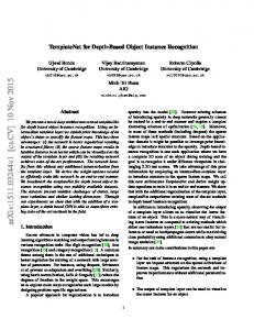
Fig. 10. Recognition accuracy as we greedily add depth kernel descriptors into the system, showing that depth image and point cloud features complement each other. (See text for details on the order of descriptors.)
of linear SVMs and the 83.8% of kernel SVMs reported in [14]. We observe that the performance of depth kernel descriptors is comparable with image kernel descriptors, which indicates that depth information is as important as visual information for category recognition. E. Analysis of Depth Kernel Descriptors We have presented five depth kernel descriptors; an important question to evaluate is whether they each add something new, and whether they are all required for object recognition. To answer this, we use a greedy strategy that incrementally adds descriptors into our system, starting with the best depth descriptor. In Fig. 10, we show the accuracy as the number of depth kernel descriptors increases in our greedy procedure. For instance recognition, the order of selected depth features are gradient, kernel PCA, size, spin and local binary pattern kernel descriptors. For category recognition, the selected depth features are gradient, spin, size, kernel PCA and local binary pattern kernel descriptors in turn. Combining all five features yields the best recognition performance. As expected, features over 3D point cloud and depth maps complement each other. VI. C ONCLUSION We have presented five depth kernel descriptors to capture different object cues including size, shape and edges. We have compared depth kernel descriptors to well known shape features, spin images, and other state-of-the-art algorithms that combine different types of features for recognition. An extensive experimental evaluation shows that our depth kernel descriptors outperform existing approaches significantly. In future work, it would be interesting to investigate whether hierarchical kernel descriptors [1] can boost the performance further.
R EFERENCES [1] L. Bo, K. Lai, X. Ren, and D. Fox. Object recognition with hierarchical kernel descriptors. In IEEE International Conference on Computer Vision and Pattern Recognition, 2011. [2] L. Bo, X. Ren, and D. Fox. Kernel Descriptors for Visual Recognition. In Advances in Neural Information Processing Systems, 2010. [3] L. Bo and C. Sminchisescu. Efficient Match Kernel between Sets of Features for Visual Recognition. In Advances in Neural Information Processing Systems, 2009. [4] Leo Breiman. Random forests. Machine Learning, 45(1):5–32, 2001. [5] Chih-Chung Chang and Chih-Jen Lin. LIBSVM: a library for support vector machines, 2001. [6] A. Coates and A. Ng. The importance of encoding versus training with sparse coding and vector quantization. In ICML, 2011. [7] J. Deng, W. Dong, R. Socher, L. Li, K. Li, and L. Fei-fei. ImageNet: A Large-Scale Hierarchical Image Database. In IEEE International Conference on Computer Vision and Pattern Recognition, 2009. [8] B. Drost, M. Ulrich, N. Navab, and S. Ilic. Model globally, match locally: Efficient and robust 3d object recognition. In IEEE International Conference on Computer Vision and Pattern Recognition, 2010. [9] F. Endres, C. Plagemann, C. Stachniss, and W. Burgard. Unsupervised discovery of object classes from range data using latent Dirichlet allocation. In Robotics: Science and Systems Conference, 2009. [10] R. Fan, K. Chang, C. Hsieh, X. Wang, and C. Lin. Liblinear: A library for large linear classification. Journal of Machine Learning Research (JMLR), 9:1871–1874, 2008. [11] G. Hinton, S. Osindero, and Y. Teh. A fast learning algorithm for deep belief nets. Neural Computation, 18(7):1527–1554, 2006. [12] A. Johnson and M. Hebert. Using spin images for efficient object recognition in cluttered 3D scenes. IEEE Transactions on Pattern Analysis and Machine Intelligence, 21(5), 1999. [13] Microsoft Kinect. http://www.xbox.com/en-us/kinect. [14] K. Lai, L. Bo, X. Ren, and D. Fox. A Large-Scale Hierarchical MultiView RGB-D Object Dataset. In IEEE International Conference on on Robotics and Automation, 2011. [15] K. Lai and D. Fox. Object Recognition in 3D Point Clouds Using Web Data and Domain Adaptation. The International Journal of Robotics Research, 2010. [16] S. Lazebnik, C. Schmid, and J. Ponce. Beyond bags of features: Spatial pyramid matching for recognizing natural scene categories. In IEEE International Conference on Computer Vision and Pattern Recognition, 2006. [17] H. Lee, R. Grosse, R. Ranganath, and A. Ng. Convolutional deep belief networks for scalable unsupervised learning of hierarchical representations. In International Conference on Machine Learning, 2009. [18] Y. Lin, F. Lv, S. Zhu, M. Yang, T. Cour, K. Yu, L. Cao, and T. Huang. Large-scale image classification: fast feature extraction and svm training. In IEEE Conference on Computer Vision and Pattern Recognition, 2011. [19] D. Lowe. Distinctive image features from scale-invariant keypoints. International Journal of Computer Vision, 60:91–110, 2004. [20] PrimeSense. http://www.primesense.com/. [21] R. Bogdan Rusu, N. Blodow, and M. Beetz. Fast point feature histograms (fpfh) for 3d registration. In IEEE International Conference on Robotics and Automation, 2009. [22] S. Shalev-Shwartz, Y. Singer, and N. Srebro. Pegasos: Primal estimated sub-gradient solver for svm. In International Conference on Machine Learning, pages 807–814. ACM, 2007. [23] J. Shotton, A. Fitzgibbon, M. Cook, T. Sharp, M. Finocchio, R. Moore, A. Kipman, and A. Blake. Real-time human pose recognition in parts from a single depth image. In IEEE International Conference on Computer Vision and Pattern Recognition, 2011. [24] B. Steder, R. B. Rusu, K. Konolige, and W. Burgard. Point feature extraction on 3d range scans taking into account object boundaries. In IEEE International Conference on on Robotics and Automation, 2011. [25] J. Wang, J. Yang, K. Yu, F. Lv, T. Huang, and Y. Guo. Localityconstrained linear coding for image classification. In IEEE International Conference on Computer Vision and Pattern Recognition, 2010. [26] Y. Bengio Y. LeCun, L. Bottou and P. Haffner. Gradient-based learning applied to document recognition. Proceedings of the IEEE, 86(11):2278–2324, 1998.