Hindawi Publishing Corporation Mathematical Problems in Engineering Volume 2013, Article ID 124263, 7 pages http://dx.doi.org/10.1155/2013/124263
Research Article Fuzzy ARTMAP Ensemble Based Decision Making and Application Min Jin,1 Zengbing Xu,2 Ren Li,2 and Dan Wu1 1 2
School of Information Science and Engineering, Hunan University, Changsha, Hunan 410082, China Sany Heavy Industry Co., Ltd., Changsha, Hunan 410100, China
Correspondence should be addressed to Min Jin;
[email protected] Received 26 July 2013; Accepted 23 August 2013 Academic Editor: Xudong Zhao Copyright © 2013 Min Jin et al. This is an open access article distributed under the Creative Commons Attribution License, which permits unrestricted use, distribution, and reproduction in any medium, provided the original work is properly cited. Because the performance of single FAM is affected by the sequence of sample presentation for the offline mode of training, a fuzzy ARTMAP (FAM) ensemble approach based on the improved Bayesian belief method is supposed to improve the classification accuracy. The training samples are input into a committee of FAMs in different sequence, the output from these FAMs is combined, and the final decision is derived by the improved Bayesian belief method. The experiment results show that the proposed FAMs’ ensemble can classify the different category reliably and has a better classification performance compared with single FAM.
1. Introduction Recently, artificial neural networks (ANNs) have been widely used as an intelligent classifier to identify the different categories based on learning pattern from empirical data modeling in complex systems [1]. For example, the BP, RBF, and SVM models have been developed quickly and utilized to classify the different fault classes of the machine equipment [2–6]. However, these traditional neural network methods have limitation on generalization, which can give rise to overfitting models for training samples. To solve the problem, the fuzzy ARTMAP (FAM) neural network is created and applied to the classification field [7–9], which is an incremental and supervised network model and designed in accordance with adaptive resonance theory. Although the FAM is able to overcome the stability-plasticity dilemma [10], in real-world application, the performance of FAM is affected by the sequence of sample presentation for the offline mode of training [11, 12]. For this drawback, some preprocessing procedures, known as the ordering algorithms such as min-max clustering and genetic algorithm [13, 14], have been proposed for FAM. Furthermore, a number of fusion techniques have been proposed for FAM to overcome this problem. Tang and Yan employed the voting algorithm of FAM to diagnose the bearings faults [15], Loo and Rao applied the multiple FAM
based on the probabilistic plurality voting strategy to medical diagnosis and classification problems [16]. Since these voting algorithms do not consider the effect of the number of the sample in each class, an improved Bayesian belief method (BBM) is used to combine multiple FAM classifiers which are offline trained in different sequence of samples in this paper. In view of the above principles, a novel ensemble FAM classifiers is proposed to improve the classification performance of single FAM. The identification schematic graph is shown in Figure 1. Firstly, through different features extraction methods, some feature parameters are extracted from the raw signals. Secondly, by the modified distance discrimination technique, the optimal feature set is selected from the original feature set. Finally, multiple FAM classifiers ensemble based on the improved BBM is employed to come up with the final classification results. The proposed method is applied to the fault diagnosis of hydraulic pump. The experiment results show the effectiveness of the proposed ensemble FAM classifiers.
2. Fuzzy ARTMAP Ensemble Using the Improved Bayesian Belief Method 2.1. Fuzzy ARTMAP (FAM). FAM consists of two ART modules, namely, ART𝑎 and ART𝑏 modules which are bridged
2
Mathematical Problems in Engineering FAMn
Data acquisition
. ..
Feature extraction
Modified distance discrimination technique
FAM3
FAM2
Improved Bayesian belief method
Classification result
FAM1
Figure 1: Flowchart of classification system. Map field Fab
ARTa F2a
ya
ab wjk
Reset
ARTb yb
xab
F2b
wja
Reset
wkb
F1a
xa
F0a
A = (a, ac )
𝜌ab
𝜌a
Match tracking
F1b
xb
F0b
B = (b, bc )
a
𝜌b
b
Figure 2: The basic structure of fuzzy ARTMAP.
via a map field [10], which is capable to forming associative maps between clusters of input domain in which ART𝑎 module functions as clustering and output domain in which the module ART𝑏 functions as clustering. Each module comprises three layers: normalization layer 𝐹0 , input layer 𝐹1 , and recognition layer 𝐹2 . The structure of FAM is shown in Figure 2. When the output domain is a finite set of class labels, FAM can be utilized as a classifier. The algorithm of FAM can be depicted simply as follows. The ART𝑎 module receives the input pattern, and the normalization of a 𝑀-dimensional input vector a, is complement-coded to a 2𝑀-dimensional vector A
When a winning category node is selected, a vigilance test (VT), namely, a similarity check against a vigilance parameter 𝜌𝑎 of the chosen category node, is taken place:
A = (a, a𝑐 ) = (𝑎1 , . . . , 𝑎𝑀, 1 − 𝑎1 , . . . , 1 − 𝑎𝑀) .
𝑤𝑗new = 𝛽 (𝐴 ∧ 𝑤𝑗old ) + (1 − 𝛽) 𝑤𝑗old ,
(1)
Then, the dimension of the input vector is kept constant: 𝑀
𝑀
𝑖=1
𝑖=1
|A| = (a, a𝑐 ) = ∑ 𝑎𝑖 + (𝑀 − ∑ 𝑎𝑖 ) = 𝑀.
(2)
Afterward, the input sample A selects the category node stored in the network by the category choice function (CCF): 𝐴 ∧ 𝑤𝑎 𝑗 = 𝑇𝑗 (𝐴) , (3) 𝑎 𝑤𝑗 + 𝛼𝑎 where ∧ is a min operator, 𝛼𝑎 is the choice function of ART𝑎 , and 𝑤𝑗𝑎 is the weight vector of the 𝑗th category node.
𝐴 ∧ 𝑤𝑗𝑎 ≥𝜌, 𝑎 |𝐴|
(4)
where 𝑤𝑗𝑎 is the winning 𝑗th node. When the above category match function (CMF) is satisfied with criterion, the resonance occurs and learning takes place; namely, the weight vector 𝑤𝑗 is updated according to the following equation: (5)
where 𝛽 ∈ [0, 1] is the learning rate. Otherwise, a new node is created in 𝐹2𝑎 which codes the input pattern. In the meantime, for the ART𝑏 the same learning algorithm occurs simultaneously using the target pattern. After the resonance occurs in the ART𝑎 and ART𝑏 , the winning node in 𝐹2𝑎 will send a prediction to ART𝑏 via the map field. The map field vigilance test is used to detect the test. If the test fails, it indicates that the winning node of ART𝑎 predicts an incorrect target class in ART𝑏 ; then a match tracking process initiates. During the match tracking, the value of 𝜌𝑎 is increased until it is slightly higher than |𝐴 ∧ 𝑤𝑗𝑎 ||𝐴|−1 ; then a new search for the other winning node
Mathematical Problems in Engineering
3
in ART𝑎 is carried out, and the process continues until the selected 𝐹2𝑎 node can make a correct prediction in ART𝑏 .
P2 P1 P5
2.2. Decision Fusion Using Bayesian Belief Method. The novel Bayesian belief method is supposed in [17]. It is based on the assumption of mutual independency of classifiers and considers the error of each classifier. Assume that in pattern space 𝑍 there are 𝑀 classes and 𝐾 classifiers. A classifier 𝑒𝑘 can be considered as a function: 𝑒𝑘 (𝑥) = 𝑗,
𝑘 = 1, 2, . . . , 𝐾,
𝑗 ∈ {1, 2, . . . , 𝑀, 𝑀 + 1} . (6)
It signifies that the sample 𝑥 is assigned to class 𝑗 by the classifier 𝑒𝑘 . And its two-dimensional confusion matrix can be represented as 𝑘 𝑛11 [ 𝑘 [𝑛 21 CM𝑘 = [ [ [ ⋅⋅⋅ 𝑘 [𝑛𝑀1
𝑘 𝑘 𝑘 𝑛12 ⋅ ⋅ ⋅ 𝑛1𝑀 𝑛1(𝑀+1)
] 𝑘 𝑘 𝑘 ] 𝑛22 ⋅ ⋅ ⋅ 𝑛2𝑀 𝑛2(𝑀+1) ], ] ⋅⋅⋅ ⋅⋅⋅ ⋅⋅⋅ ⋅⋅⋅ ] 𝑘 𝑘 𝑘 𝑛𝑀2 𝑛𝑀𝑀 𝑛𝑀(𝑀+1) ]
(𝑘 = 1, . . . , 𝐾) ,
(7) which is obtained by executing 𝑒𝑘 (𝑥) on the test data set after 𝑒𝑘 (𝑥) is trained. Each row 𝑖 corresponds to class 𝑐𝑖 and each column 𝑗 corresponds to 𝑒𝑘 (𝑥) = 𝑗. The matrix unit 𝑛𝑖𝑗𝑘 means the input samples from class 𝑐𝑖 while are assigned to class 𝑐𝑗 by classifier 𝑒𝑘 (𝑥). The number of samples in class 𝑐𝑖 is 𝑛𝑖.𝑘 = 𝑘 ∑𝑀+1 𝑗=1 𝑛𝑖𝑗 , where 𝑖 = 1, . . . , 𝑀, and the number of samples
𝑘 labeled 𝑗 by 𝑒𝑘 (𝑥) is 𝑛.𝑗𝑘 = ∑𝑀 𝑖=1 𝑛𝑖𝑗 , where 𝑗 = 1, . . . , 𝑀 + 1. Considering the difference of the number of samples in each class, on the basis of the confusion matrix a belief measure of classification can be calculated for each classifier by the following belief function [18]: 𝑘 𝑛𝑖𝑗𝑘 / ∑𝑀+1 𝑐𝑖 𝑐𝑖 𝑗=1 𝑛𝑖𝑗 , ) = 𝑃 (𝑥 ∈ = 𝑗) = 𝑀 𝑘 𝑒𝑘 (𝑥) 𝑒𝑘 (𝑥) ∑𝑖=1 (𝑛𝑖𝑗𝑘 / ∑𝑀+1 𝑗=1 𝑛𝑖𝑗 )
𝑖 = 1, 2, . . . , 𝑀,
P4
Figure 3: The schematic diagram of the experimental setup.
Thus, 𝑥 is classified into a class 𝑗 (𝑗 = 1, 2, . . . , 𝑀 + 1) according to the belief of making the final decision Bel(𝑗) = max𝑀+1 𝑖=1 𝐵(𝑖).
3. Case Study
𝑀 + 1 is an unknown label
𝐵𝑘 (𝑥 ∈
P3
𝑗 = 1, 2, . . . , 𝑀+1. (8)
When multiple classifiers 𝑒1 , 𝑒2 , . . . , 𝑒𝑘 are developed, their correspondent beliefs 𝐵1 , 𝐵2 , . . . , 𝐵𝑘 are computed based on the performance of base classifiers. Combining the belief measures of all fusion classifiers can result in the final belief measure of the multiple classifier system. In case of equal a priori class probabilities, the combination rule can be depicted as follows: 𝐵 (𝑖) = 𝐵 (𝑥 ∈ 𝑐𝑖 | 𝑒1 (𝑥) , 𝑒2 (𝑥) , . . . , 𝑒𝑘 (𝑥) , EN)
In order to evaluate the effectiveness of the supposed ensemble FAM, the fault identification of hydraulic pump is taken as example. Figure 3 shows the schematic diagram of experiment rig. Four accelerometers are attached to the housing with magnetic bases and mounted at the positions P1, P2, P3, and P4. Pressure sensor is mounted at the position P5. Considering the sensitivity to the fault conditions of hydraulic pump, the vibration signal which is acquired by the accelerometer at the position P2 is utilized to identify the fault categories. And the vibration signals are acquired, respectively, under normal condition and the different fault conditions, such as inner plunger wear, inner race wear, ball wear, swashplate wear, portplate wear, and paraplungers wear. 3.1. Data Preparation. The data set contains 490 samples. These data samples are divided into 245 training and 245 test samples. The detailed descriptions of three data sets are shown in Table 1. In order to identify the different fault categories, a seven-class classification problem need be solved. 3.2. Feature Extraction and Selection 3.2.1. Feature Extraction. Feature parameters are used to characterize the information relevant to the conditions of the hydraulic pump. To acquire more fault-related information, many features in different symptom domains are extracted from the measured signals. Frequency domain is another description of a signal. In [19], some novel features which can give a much fuller picture of the frequency distribution in each band of frequencies are proposed. Supposed 𝑁 points of normalized PSD, 𝑃𝑥𝑥 , of the vibration signal, 𝑃𝑥𝑥 are divided into 𝐿 segments, where 𝐿 is 1 in this study. The four features based on the moment estimates of power can be obtained as follows:
= 𝑃 (𝑥 ∈ 𝑐𝑖 | 𝑒1 (𝑥) , 𝑒2 (𝑥) , . . . , 𝑒𝑘 (𝑥) , EN) =
∏𝐾 𝑘=1 𝐵𝑘 (𝑥 ∈ 𝑐𝑖 | 𝑒1 (𝑥) , EN)
∑ 𝑖 ∏𝐾 𝑘=1 𝐵𝑘 (𝑥 ∈ 𝑐𝑖 | 𝑒1 (𝑥) , EN)
,
𝑘1 =
𝑖 = 1, 2, . . . , 𝑀 + 1. (9)
𝑘2 =
1 ∑ 𝑃 (𝑛) , 𝑁 𝑁 𝑥𝑥
2 1 ∑ (𝑃 (𝑛) − 𝑘1 ) , 𝑁 − 1 𝑁 𝑥𝑥
4
Mathematical Problems in Engineering Table 1: Sample subset statistics.
The number The number of training of test samples samples 45 30 25 50 20 40 35
45 30 25 50 20 40 35
𝑘3 = 𝑘4 =
1 𝑁 𝑘23/2
Operation condition
Label of classification
Normal Inner plunger wear Inner race wear Ball wear Swashplate wear Portplate wear Paraplungers wear
1 2 3 4 5 6 7
In addition, due to sensitiveness of these model parameters to the shape of the vibration data, AR model parameters are utilized to characterize the information about the conditions of hydraulic pumps. The AR model is written as follows: 𝑥𝑡 = 𝜙1 𝑥𝑡−1 + 𝜙2 𝑥𝑡−2 + ⋅ ⋅ ⋅ + 𝜙𝑝 𝑥𝑡−𝑝 ,
where 𝑥𝑡−1 , 𝑥𝑡−2 , . . . , 𝑥𝑡−𝑝 are the 𝑟 previous samples, 𝑥𝑡 is the predicted sample of the signal, and 𝜙1 , 𝜙2 , . . . , 𝜙𝑡−𝑝 is AR model parameters, which can be obtained by the least square method in [21] and expressed by the following formula: −1 𝜙̂ = (𝑋𝑇 𝑋) 𝑋𝑇𝑌,
∑ (𝑃𝑥𝑥 (𝑛) − 𝑘1 ) ,
𝑥𝑛 𝑥𝑛−1 ⋅ ⋅ ⋅ 𝑥1 [ 𝑥𝑛+1 𝑥𝑛 ⋅ ⋅ ⋅ 𝑥2 ] [ ] 𝑋=[ ], .. [ ] . [𝑥𝑁−1 𝑥𝑁−2 ⋅ ⋅ ⋅ 𝑥𝑁−𝑛 ]
𝑁
(10) where “𝑛” is the number of total data points and 𝑁 is the number of sample points in the lth segment. In order to characterize the spectrum with a higher accuracy, the moment estimates of frequency weighed by power are calculated by the following formulas: 1 ∑ 𝑓 (𝑛) 𝑃𝑥𝑥 (𝑛) , 𝐾𝑙 𝑁 2
∑𝑁 [(𝑓 (𝑛) − 𝑘5 ) 𝑃𝑥𝑥 (𝑛)] 𝐾𝑙
,
1 3 𝑘7 = ∑ [(𝑓 (𝑛) − 𝑘5 ) 𝑃𝑥𝑥 (𝑛)] , 3 𝐾𝑙 𝑘6 𝑁 𝑘8 =
(11)
1 4 ∑ [(𝑓 (𝑛) − 𝑘5 ) 𝑃𝑥𝑥 (𝑛)] , 𝐾𝑙 𝑘64 𝑁
where 𝑓(𝑛) is the corresponding frequency of 𝑃𝑥𝑥 (𝑛) and 𝐾𝑙 is the total power in the segment. Then, the total number of features extracted for each spectrum is 1 × 8. To depict the fault-related information about the hydraulic pumps quantitatively, the first-order continuous wavelet grey moment (WGM) [20] of vibration signal is extracted. Assuming the wavelet coefficients matrix [𝑊]𝑀×𝑁 which can be displayed by the continuous wavelet transform (CWT) scalogram, 𝑀 and 𝑁 are the scales and the time of the scalogram, respectively, the matrix [𝑊]𝑀×𝑁 is divided into 𝑚 parts along the scale equally, and the first-order wavelet grey moment 𝑔1 of each part can be calculated by the following equation: 𝑔1 =
𝑀/𝑚
𝑁 1 2 ∑ ∑ 𝑤𝑖𝑗1 √(𝑖 − 1)2 + (𝑗 − 1) , (𝑀/𝑚) × 𝑁 𝑖=1 𝑗
(12)
where 𝑤𝑖𝑗 is the element of matrix [𝑊](𝑀/𝑚)×𝑁. In this paper, the 𝑚 is set as 8 and the wavelet function is Morlet wavelet.
(15)
𝑇
𝑌 = [𝑥𝑛+1 , 𝑥𝑛+2 , . . . , 𝑥𝑁] .
𝑘6 = √
(14)
where 3
1 4 ∑ (𝑃 (𝑛) − 𝑘1 ) , 𝑁 𝑘22 𝑁 𝑥𝑥
𝑘5 =
(13)
In this study, the parameter 𝑝 is set as 8. Thus, 24 features constitute the original feature set. 3.2.2. Feature Selection. In order to improve the identification accuracy and reduce the computation burden, some sensitive features providing characteristic information for the classification system need to be selected, and irrelevant or redundant features must be removed. In this study, based on [22], a modified distance discriminant technique is employed to select the optimal features. Supposing that a feature set of 𝐽 classes consists of 𝑁 samples, in the 𝑗th class there are 𝑁𝑗 samples, where 𝑗 = 1, 2, . . . , 𝐽, and 𝑁 = ∑𝐽𝑗=1 𝑁𝑗 . Each sample is represented by 𝑀 features, and the 𝑚th feature of the 𝑖th sample is written as 𝑓𝑖𝑚 . Then, the feature selection process can be described as follows. Step 1. Calculate the standard deviation and the mean of all samples in the 𝑚th feature: 2 = 𝜎𝑚
𝑚 2 1 𝑁 𝑚 ∑ (𝑓𝑖 − 𝑓 ) , 𝑁 𝑖=1
𝑚
𝑓 =
1 𝑁 𝑚 ∑𝑓 . 𝑁 𝑖=1 𝑖
(16)
Step 2. Calculate the standard deviation and the mean of the sample in the 𝑗th class in the 𝑚th feature, respectively, 2 𝜎𝑚 (𝑗) =
𝑁𝑗
𝑚 2 1 ∑ (𝑓𝑗𝑚 − 𝑓𝑗 ) , 𝑁𝑗 − 1 𝑗=1
𝑚
𝑓𝑗 =
𝑁𝑗
1 ∑ 𝑓𝑚 . 𝑁𝑗 𝑗=1 𝑗 (17)
Step 3. Calculate the weighted standard deviation of the class center 𝑔𝑗 in the 𝑚th feature: 𝐽
2
2 𝜎𝑚 = ∑ 𝜌𝑗 (𝑔𝑗𝑚 − 𝑔𝑚 ) = 𝜇1 − 𝜇22 , 𝑗=1
(18)
Mathematical Problems in Engineering
5
where 𝜇1 = ∑𝐽𝑗=1 𝜌𝑗 (𝑔𝑗𝑚 )2 , 𝜇2 = ∑𝐽𝑗=1 𝜌𝑗 𝑔𝑗𝑚 , 𝑔𝑚 = ∑𝐽𝑗=1 𝜌𝑗 𝑔𝑗𝑚 , and 𝑔𝑚 are the centers of all samples in the 𝑚th feature; 𝑔𝑗𝑚 is the center of the samples of the 𝑗th class in the 𝑚th feature; 𝜇1 , 𝜇2 are the weighted means of the squared class center 𝑔𝑗2 and the class center 𝑔𝑗 in the 𝑚th feature; 𝜌𝑗 is the prior probability of the 𝑗th class, respectively; and ∑𝐽𝑗=1 𝜌𝑗 = 1. Step 4. Calculate the distance discriminant factor of the 𝑚th feature: 𝑚 = 𝑑𝑏𝑚 − 𝛽𝑑𝑤
𝐽 1 [ 2 2 − 𝛽 𝜌𝑗 𝜎𝑚 (𝑗)] , 𝜎 ∑ 𝑚 2 𝜎𝑚 𝑗=1 ] [
(19)
where 𝑑𝑏𝑚 is the distance of the 𝑚th feature between different 𝑚 corresponds to the distance of the 𝑚th feature classes, 𝑑𝑤 𝑚 , within classes, and 𝛽 is used to control the impact of 𝑑𝑤 which is set as 2 in this paper. Considering the overlapping degree among different classes, a compensation factor is calculated as follows. 𝑚 in Firstly, define and calculate the variance factor of 𝑑𝑤 the 𝑚th feature as follows: 𝑚 = V𝑤
𝑚 ) max (𝑑𝑤 . 𝑚 min (𝑑𝑤 )
(20)
Secondly, define and calculate the variance factor of 𝑑𝑏𝑚 in the 𝑚th feature as follows: 𝑚 𝑚 max 𝑓𝑖 − 𝑓𝑗 𝑢𝑏𝑚 = 𝑚 𝑚 , min 𝑓𝑖 − 𝑓𝑗 (21) 𝑚
𝑚
(𝑓𝑖 − 𝑓𝑗 ) 𝑚 𝑚 , 𝑓𝑖 − 𝑓𝑗 = 2 𝜎𝑚
𝑖, 𝑗 = 1, 2, . . . , 𝐽, 𝑖 ≠ 𝑗.
Then, the compensation factor of the 𝑚th feature can be defined and calculated as follows: 𝜂𝑚 =
1 1 + 𝑚. 𝑚 V𝑤 𝑢𝑏
(22)
Thus, the modified distance discriminant factor can be calculated as follows: 𝑚 𝑚 𝑑𝑏𝑚 − 𝛽 𝑑𝑤 = 𝑑𝑏𝑚 − (𝛽𝜂𝑚 ) 𝑑𝑤
=
𝐽 1 [ 2 1 1 2 𝜎𝑚 − 𝛽∑ ( 𝑤 + 𝑏 ) 𝜌𝑗 𝜎𝑚 (𝑗)] , (23) 2 𝜎𝑚 V 𝑢 𝑗 𝑗=1 𝑗 ] [
(𝑚 = 1, 2, . . . , 𝑀) . Step 5. Rank 𝑀 features in descending order according to 2 2 the modified distance discriminant factors (1/𝜎𝑚 )[𝜎𝑚 − 2 𝛽((1/V𝑗𝑤 ) + (1/𝑢𝑗𝑏 )) ∑𝐽𝑗=1 𝜌𝑗 𝜎𝑚 (𝑗)] = 𝜆 𝑚 ; then normaliz 𝜆 𝑚 by 𝜆𝑚 = (𝜆 𝑚 − min(𝜆 𝑚 ))/(max(𝜆 𝑚 ) − min(𝜆 𝑚 )) and get the distance discriminant criteria. Clearly, bigger 𝜆𝑚 (𝑚 = 1, 2, . . . , 𝑀) signifies that the correspondent feature is better to separate 𝐽 classes.
Step 6. Set a threshold value 𝛾 and select the sensitive features whose distance discriminant factor 𝜆𝑚 ≥ 𝛾 from the set of 𝑀 features. 3.3. Diagnosis Analysis. It is well known that the data-ordering of training samples can affect the classification accuracy of single FAM, and that a single output used to represent multiple classes may lead to lower classification accuracy. In order to know how well the proposed FAMs’ ensemble work, that is, how significant the generalization ability is improved by utilizing the improved Bayesian belief method to combine the classification results from a committee of single FAM trained with different data-ordering of training samples, the performance of single FAM is also conducted. In the diagnosis phase performed by the single FAM and FAM ensemble, they are all trained in the fast learning and conservative mode (i.e., setting 𝛽 = 1 in (5) and 𝛼𝑎 = 0.001 in (3)). Besides, in order to ensure the performance of stabilityplasticity, the vigilance parameter of FAM is set as 𝜌𝑎 = 0.5, and the ensemble size is set as 5. In order to improve the classification accuracy and reduce the computation time, in each case some salient features are selected from each feature set by the modified distance discriminant technique, respectively, and then input into the five single FAM in different sequence in the process of training. Figure 4 shows the modified distance discriminant factor 𝜆𝑚 of all features in the feature sets. From the figure it can be seen that the threshold 𝛾 corresponding to the optimal features are different for the case. That is to say, the number of salient features is different. Figure 5 summarizes the classification results in terms of test accuracy of single FAM and FAMs’ ensemble. From the figure, it can be seen that the FAMs’ ensemble (0.988) outperforms the single FAMs’ in terms of accuracy. And the test accuracy is getting higher when the number of single FAM increases. These indicate that FAMs’ ensemble can identify the different fault categories of hydraulic pump well. 3.3.1. Effect of Different Threshold for Feature Selection. As shown in Figure 4, when the threshold value 𝛾 is set properly, some redundant and irrelevant features can be removed from the original feature set. To test the effect of the proposed feature selection method based on the modified distance discriminant technique, a series of experiments is carried out against the threshold value 𝛾, in which the parameter of the single FAM is the same as the above, and the size of ensemble FAM is set as 5. Figure 6 lists the classification accuracy of five individual FAMs’ and FAM ensemble against the different thresholds. From the figure, it can be noticed that when 𝛾 = 0 (original feature set), the test accuracy of single FAM and FAM ensemble is 0.824 and 0.845, respectively. The highest test accuracy of single FAM and FAMs’ ensemble (0.915 and 0.988) is arrived synchronously when 𝛾 = 0.8, where the optimal feature set is selected. However, when the threshold value continues to increase, the test accuracy of single FAM and FAMs’ ensemble tends to decrease. And when threshold 𝛾 > 0.9, the test accuracy of single FAM and FAMs’ ensemble
Mathematical Problems in Engineering
Distance discrimination factor
6
Table 2: Test accuracy produced by different classification methods.
1
Method 𝛾 = 0.8
0.5
0
0
5
10
15
20
25
Feature Original features Selected features
Figure 4: Feature selection for three different data sets.
Accuracy
1
0.95
0.9 1
1.5
2
2.5 3 3.5 4 Number of fused classifiers
4.5
5
Figure 5: Relationship between the test accuracy and the number of single FAM used in FAMs’ ensemble.
0.95 0.9 Test accuracy
91.5 98.8 95.2
by FAMs’ ensemble and single FAM are compared with those produced by other classification methods. In this experiment, the parameters of FAM ensemble and single FAM are the same as the above. Table 2 shows the test results of the FAMs’ ensemble versus other classification methods. From the table it can be seen that the average test accuracy using single FAMs’ is the lowest. However, the test accuracy produced by two FAMs’ ensemble methods is higher than that produced by the single classifier, and the test success rate of the proposed FAMs’ ensemble is highest and higher than that of FAM ensemble with voting algorithm. These indicate that the proposed FAMs’ ensemble has comparatively superior diagnosis performance.
4. Conclusions The classification performance of FAM is affected by the sequence of training samples. A novel and reliable FAMs’ ensemble based on the improved Bayesian belief method is described and proposed to improve the classification performance of FAM in this paper, which combines the output from a committee of FAM fed with different orderings of training samples and derives the combined decision. And the supposed FAMs’ ensemble method is applied to the fault identification of hydraulic pump. The experiment results testify that the proposed FAM ensemble can diagnose the fault categories accurately and reliably and has better diagnosis performance compared with single FAM. These indicate that the proposed FAMs’ ensemble has a good promise in the engineering of classification and decision making.
1
0.85 0.8 0.75 0.7
Single FAM The proposed FAM ensemble FAMs’ ensemble with voting algorithm and five FAMs
Test accuracy (%)
0
0.1
0.2
0.3
0.4 0.5 0.6 Threshold 𝛾
0.7
0.8
0.9
1
Accuracy of single FAM Accuracy of FAMs’ ensemble
Figure 6: Classification accuracy comparison for different threshold.
is lower than that used in all features with threshold 𝛾 = 0. This is mainly because the smaller number of features leads to the overfitting; namely, the drastic reduction of features can lead to a decrease in the test accuracy. 3.3.2. Classification Performance Comparison with Other Classification Methods. In order to test the superiority of the proposed FAMs’ ensemble method, the test results produced
Acknowledgments This work is supported by the National Scientific and Technological Achievement Transformation Project of China (Grant no. 201255), Electronic Information Industry Development Fund of China (Grant no. 2012407), the National Natural Science Foundation of China (Grant no. 61374172), and the Fundamental Research Funds for the Central Universities, Hunan University, China.
References [1] M. M. Polycarpou and A. J. Helmicki, “Automated fault detection and accommodation: a learning systems approach,” IEEE Transactions on Systems, Man and Cybernetics, vol. 25, no. 11, pp. 1447–1458, 1995.
Mathematical Problems in Engineering [2] X. Dong, L. Qiu, and Z. Wang, “On line condition monitoring and fault diagnosis for hydraulic pump based on BP algorithm,” Journal of Beijing University of Aeronautics and Astronautics, vol. 23, no. 3, pp. 322–327, 1997. [3] Y. H. Jia, Y. G. Kong, and S. P. Liu, “Application of wavelet neural network to fault diagnosis of hydraulic pumps,” in Proceedings of the 6th International Symposium on Test and Measurement, pp. 19–22, 2005. [4] H. Liu, S. Wang, and P. Ouyang, “Fault diagnosis based on wavelet package and Elman neural network for a hydraulic pump,” Journal of Beijing University of Aeronautics and Astronautics, vol. 33, no. 1, pp. 67–71, 2007. [5] F. Sun and Z. Wei, “Rolling bearing fault diagnosis based on wavelet packet and RBF neural network,” in Proceedings of the 26th Chinese Control Conference (CCC ’07), pp. 451–455, July 2007. [6] B. Samanta, K. R. Al-Balushi, and S. A. Al-Araimi, “Artificial neural networks and support vector machines with genetic algorithm for bearing fault detection,” Engineering Applications of Artificial Intelligence, vol. 16, no. 7-8, pp. 657–665, 2003. [7] R. Javadpour and G. M. Knapp, “A fuzzy neural network approach to machine condition monitoring,” Computers and Industrial Engineering, vol. 45, no. 2, pp. 323–330, 2003. [8] S. C. Tan and C. P. Lim, “Application of an adaptive neural network with symbolic rule extraction to fault detection and diagnosis in a power generation plant,” IEEE Transactions on Energy Conversion, vol. 19, no. 2, pp. 369–377, 2004. [9] X. Zhao, L. Zhang, P. Shi, and H. Karimi, “Novel stability criteria for T-S fuzzy systems,” IEEE Transactions on Fuzzy Systems, vol. 99, pp. 110–111, 2013. [10] G. A. Carpenter, S. Grossberg, N. Markuzon, J. H. Reynolds, and D. B. Rosen, “Fuzzy ARTMAP: a neural network architecture for incremental supervised learning of analog multidimensional maps,” IEEE Transactions on Neural Networks, vol. 3, no. 5, pp. 698–712, 1992. [11] M. Georgiopoulos, H. Fernlund, G. Bebis, and G. L. Heileman, “Order of search in fuzzy ART and fuzzy ARTMAP: effect of the choice parameter,” Neural Networks, vol. 9, no. 9, pp. 1541–1559, 1996. [12] M. Jin, X. Zhou, Z. M. Zhang, and M. M. Tentzeris, “Shortterm power load forecasting using grey correlation contest modeling,” Expert Systems with Applications, vol. 39, no. 1, pp. 773–779, 2012. [13] I. Dagher, M. Georgiopoulos, G. L. Heileman, and G. Bebis, “An ordering algorithm for pattern presentation in fuzzy ARTMAP that tends to improve generalization performance,” IEEE Transactions on Neural Networks, vol. 10, no. 4, pp. 768–778, 1999. [14] R. Palaniappan and C. Eswaran, “Using genetic algorithm to select the presentation order of training patterns that improves simplified fuzzy ARTMAP classification performance,” Applied Soft Computing Journal, vol. 9, no. 1, pp. 100–106, 2009. [15] Z. Tang and X. Yan, “Voting algorithm of fuzzy ARTMAP and its application to fault diagnosis,” in Proceedings of the 4th International Conference on Fuzzy Systems and Knowledge Discovery (FSKD ’07), pp. 535–538, August 2007. [16] C. K. Loo and M. V. C. Rao, “Accurate and reliable diagnosis and classification using probabilistic ensemble simplified fuzzy ARTMAP,” IEEE Transactions on Knowledge and Data Engineering, vol. 17, no. 11, pp. 1589–1593, 2005. [17] L. Lam and C. Y. Suen, “Optimal combinations of pattern classifiers,” Pattern Recognition Letters, vol. 16, no. 9, pp. 945– 954, 1995.
7 [18] L. Chen and H. L. Tang, “Improved computation of beliefs based on confusion matrix for combining multiple classifiers,” Electronics Letters, vol. 40, no. 4, pp. 238–239, 2004. [19] M. L. D. Wong, L. B. Jack, and A. K. Nandi, “Modified selforganising map for automated novelty detection applied to vibration signal monitoring,” Mechanical Systems and Signal Processing, vol. 20, no. 3, pp. 593–610, 2006. [20] Z. Yanping, H. Shuhong, H. Jinghong, S. Tao, and L. Wei, “Continuous wavelet grey moment approach for vibration analysis of rotating machinery,” Mechanical Systems and Signal Processing, vol. 20, no. 5, pp. 1202–1220, 2006. [21] S. Z. Yang, Y. Wu, and J. P. Xuan, Time Series Analysis in Engineering Application, Huazhong University of Science and Technology Press, Wuhan, China, 2007. [22] J. Liang, S. Yang, and W. Adam, “Invariant optimal feature selection: a distance discriminant and feature ranking based solution,” Pattern Recognition, vol. 41, no. 5, pp. 1429–1439, 2008.
Advances in
Operations Research Hindawi Publishing Corporation http://www.hindawi.com
Volume 2014
Advances in
Decision Sciences Hindawi Publishing Corporation http://www.hindawi.com
Volume 2014
Journal of
Applied Mathematics
Algebra
Hindawi Publishing Corporation http://www.hindawi.com
Hindawi Publishing Corporation http://www.hindawi.com
Volume 2014
Journal of
Probability and Statistics Volume 2014
The Scientific World Journal Hindawi Publishing Corporation http://www.hindawi.com
Hindawi Publishing Corporation http://www.hindawi.com
Volume 2014
International Journal of
Differential Equations Hindawi Publishing Corporation http://www.hindawi.com
Volume 2014
Volume 2014
Submit your manuscripts at http://www.hindawi.com International Journal of
Advances in
Combinatorics Hindawi Publishing Corporation http://www.hindawi.com
Mathematical Physics Hindawi Publishing Corporation http://www.hindawi.com
Volume 2014
Journal of
Complex Analysis Hindawi Publishing Corporation http://www.hindawi.com
Volume 2014
International Journal of Mathematics and Mathematical Sciences
Mathematical Problems in Engineering
Journal of
Mathematics Hindawi Publishing Corporation http://www.hindawi.com
Volume 2014
Hindawi Publishing Corporation http://www.hindawi.com
Volume 2014
Volume 2014
Hindawi Publishing Corporation http://www.hindawi.com
Volume 2014
Discrete Mathematics
Journal of
Volume 2014
Hindawi Publishing Corporation http://www.hindawi.com
Discrete Dynamics in Nature and Society
Journal of
Function Spaces Hindawi Publishing Corporation http://www.hindawi.com
Abstract and Applied Analysis
Volume 2014
Hindawi Publishing Corporation http://www.hindawi.com
Volume 2014
Hindawi Publishing Corporation http://www.hindawi.com
Volume 2014
International Journal of
Journal of
Stochastic Analysis
Optimization
Hindawi Publishing Corporation http://www.hindawi.com
Hindawi Publishing Corporation http://www.hindawi.com
Volume 2014
Volume 2014