07-095.qxd
11/12/08
12:07 PM
Page 1573
Fuzzy ARTMAP Based Neurocomputational Spatial Uncertainty Measures Zhe Li
Abstract This paper proposes non-parametric measures for the fuzzy ARTMAP computational neural network to handle spatial uncertainty in remotely sensed imagery classification, i.e., ART Commitment (ART-C) and ART Typicality (ART-T), expressing in the first case the degree of commitment a classifier has for each class for a specific pixel, and in the second case, how typical that pixel’s reflectances are of the ones upon which the classifier was trained for each class. Results from case studies were compared against the previously developed SOM Commitment (SOM-C) and SOM Typicality (SOM-T) classifiers as well as conventional Bayesian posterior probability and Mahalanobis typicality soft classifiers. Principal Components Analysis (PCA) was used to explore the relationship between these different measures. Results indicate that ART-C and SOM-C measures express values similar to Bayesian posterior probabilies, and ART-T and SOM-T are closely related to Mahalanobis typicalities. However, the proposed neural approaches outperform the traditional methods due to their non-parametric advantage.
Introduction Recently, soft classification has become an attractive means of land-cover classification from remotely-sensed imagery (Bernard et al., 1997). Conventional hard classification, which assumes that each pixel represents a homogeneous land-cover, has been widely used for land-cover mapping. In reality, a pixel may represent mixed classes or unknown patterns. The “one-pixel-one-class” method no doubt causes information loss (Wang, 1990) and fails to depict heterogeneity and variability within the pixel. Rather than forcing allocation to one class, in contrast, soft classification yields a set of images expressing information of the membership, probability, or sub-pixel mixture proportion of each land-cover class (Eastman and Laney, 2002; Foody, 1996). Soft classifiers are used not only for the potential of uncovering the proportional constituents of mixed pixels (Foody, 1999), but also for the examination of classification uncertainty (Eastman and Laney, 2002). Much effort has been directed in the last two decades to develop soft classification algorithms for remotely sensed data, which include soft outputs based on Bayesian posterior probabilities (Foody, 1992; Eastman and Laney, 2002), Mahalanobis typicalities (Foody et al., 1992), Fuzzy Set membership grades (Eastman, 2003), Linear Mixture fractions (Settle and Drake, 1993), Dempster-Shafer beliefs
Spatial Information Technology Specialist Research Program East-West Center, 1601 East-West Road, Honolulu, HI 96848, and formerly with the GISc Center of Excellence, South Dakota State University, Brookings, SD and the Graduate School of Geography, Clark University, Worcester, MA (
[email protected]). PHOTOGRAMMETRIC ENGINEERING & REMOTE SENSING
(Eastman et al., 2005), and Neural Networks activation levels (Atkinson et al., 1997; Zhang and Foody, 2001). Conventional soft classifiers such as those based on Bayesian and Mahalanobis constructs are parametric and limited by the assumptions about the form and distribution of input data (Foody et al., 1992). In recent years, machine learning algorithms have emerged as effective non-parametric alternatives to conventional parametric algorithms when dealing with complex measurement spaces. Among machine learning techniques, there has been considerable interest in the use of neural networks for the classification of remotely sensed imagery due to their numerous advantages over conventional classifiers, such as no assumptions about the form and distribution of input data, non-linear decision boundaries and the capabilities of generalizing inputs, and learning of complex patterns (Foody, 1996, 1997, 1998, and 1999; Atkinson et al., 1997; Liu et al., 2003; Tso and Mather, 2001). From the range of neural network types, the Multi-Layer Perceptron (MLP) network trained with the back-propagation algorithm is the most frequently used model in remote sensing image classification (Foody, 2004). In theory, it can approximate virtually any function of interest to any desired degree of accuracy (Hornik et al., 1989) and is capable of producing both hard and soft outputs. However, due to its heuristic characteristics, there is not a universally acceptable rule for the selection of an appropriate network topology and learning properties (Zhang et al., 2001; Tso et al., 2001; Foody, 2004; Qiu, 2004). Moreover, a MLP is not able to incorporate new information without forgetting past learning (Carpenter, 1989). Although there have been improvements in the use of MLP (Foody, 2004), attention has been increasingly focused on other machine learning techniques such as Radial Basis Function networks (RBF) (Rollet et al., 1998; Foody, 2004), Kohonen’s Self-Organizing Map (SOM) (Kohonen, 1990 and 2001; Ji, 2000; Villmann et al., 2003), Hopfield networks (Tatem, 2002 and 2003), pattern recognition techniques based on Adaptive Resonance Theory (ART/ARTMAP) (Carpenter et al., 1992; Rohwer et al., 1994; Tso et al., 2001) and Decision Tree classifiers (Breiman et al., 1984; Hansen et al., 1996; Simard et al., 2002; Pal and Mather, 2003). Among all these models, fuzzy ARTMAP (Carpenter et al., 1992) is a particularly interesting configuration and shows significant promise in the classification of remotely sensed imagery. For example, Mannan et al. (1998) found that fuzzy ARTMAP was more efficient than MLP with the back propagation learning in supervised classification of multi-spectral remotely sensed images. However, the fuzzy
Photogrammetric Engineering & Remote Sensing Vol. 74, No. 12, December 2008, pp. 1573–1584. 0099-1112/08/7412–1573/$3.00/0 © 2008 American Society for Photogrammetry and Remote Sensing D e c e m b e r 2 0 0 8 1573
07-095.qxd
11/12/08
12:07 PM
Page 1574
ARTMAP neural network has not been explored as thoroughly as other neural network models, although some experiments were conducted (Mannan et al., 1998; Gopal et al., 1999; Seto and Liu, 2003; Stathakis and Vasilakos, 2006). Both the Self-Organizing Map (SOM) and fuzzy ARTMAP neural network are trained based upon a competitive mechanism and use the “winner-take-all” rule. This allows generic soft classification algorithms to be developed for both the two models. This paper is an extension of a previous study on the commitment and typicality measures for the Self-Organizing Map (Li, 2007; Li and Eastman, 2006) and is concerned with the development of soft classification procedures for the fuzzy ARTMAP neural network model. Although a few studies have explored mixed pixel analysis using fuzzy ARTMAP (Carpenter et al., 1999; Liu et al., 2004; Liu et al., 2004), soft classification for uncertainty analysis has not been undertaken. The objective of this study is to develop soft classification algorithms for the fuzzy ARTMAP neural network model, i.e., ART Commitment and ART Typicality to handle uncertainty analysis in remotely sensed image classification.
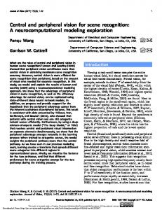
input layer neurons are doubled to accommodate the 2n elements, i.e., {x1, x2, . . . xn, 1⫺x1, 1⫺x2, . . . 1⫺xn}. The number of F2 layer neurons of fuzzy ART is dynamically determined, i.e., the F2 layer begins with a single neuron and dynamically increases the number during the process of learning (Mannan et al., 1998). Fuzzy ARTMAP, designed for supervised classification, has two additional layers, i.e., a map field layer and an output layer. The latter makes up the ARTB model. The map field layer connects the ARTA and ARTB models. The output and map field layers consist of m neurons each, where M is the output class dimension. There exists a one-to-one connection between these two layers. Figure 1 illustrates the basic architecture of a fuzzy ARTMAP model. During the unsupervised training stage of the fuzzy ARTMAP, every input pattern is compared with existing clusters. An F2 neuron will be selected as a winner (often known as being “committed”) if it is similar enough to the input pattern. The winner is determined using a fuzzy intersection operation1 ,i.e.: n
An Overview of the Fuzzy ARTMAP Procedure Adaptive Resonance Theory (ART)-based neural networks have evolved from the biological theory of cognitive information processing and have been developed by Grossberg (1976) and Carpenter (1991). ART networks are designed, in particular, to resolve the stability-plasticity dilemma: they are stable enough to preserve significant past learning, but nevertheless remain adaptable enough to incorporate new information whenever it might appear (Carpenter, 1989). A comprehensive description of ART models is detailed in the literature (Carpenter et al., 1991, 1992; Mannan et al., 1998; Gamba and Dell’Aqua, 2003). Fuzzy ART is a clustering algorithm for unsupervised classification and can take either analogue or binary input signals. It contains two layers, i.e., F1 (input layer) and F2 (category layer). These two layers make up the ARTa model (Figure 1). The F1 layer represents the input feature vector and thus has neurons for each measurement dimension. Fuzzy ART contains 2n inputs for the complement coded input feature vector to preserve amplitude information (Carpenter et al., 1991) For example, if an n-dimensioned vector x {x1, x2, . . . xn} is presented to the network, the number of the
Winner ⫽ arg max j
兩xi wji 兩
冢 a ⫹兩w 兩 冣 ⫽ arg max j
ji
兺 min(xi,wji) i⫽1 n
a ⫹ 兺 wji
(1)
i⫽1
where xi is the input pattern, and wji is the connecting weight between the F1 and F2 layer; the term in parentheses is the choice function, and a is the choice parameter. Once the winner is determined (committed), it is subject to a vigilance test according to: n
兺 min(xi, wji) i⫽1 n
兺 xi
ⱖr
(2)
i⫽1
where r is the vigilance parameter, a predefined positive number. If the test in the above equation fails, this winner is considered invalid and ruled out (reset) and the search is repeated until a new satisfactory winner is found (resonance). If no winner is selected, a new neuron will be generated to accommodate this input pattern. Carpenter (1989) gave a vivid analogy that the category choice can be conceived as a hypothesis, whilst the vigilance test is similar to a statistical significant test. When a winner is selected (a resonance is found), weights connecting it with the F1 neurons are updated as: w jit⫹1 ⫽ b(xi w jit ) ⫹ (1 ⫺ b)w jit
(3)
where b is the learning rate between F1 layer and F2 layer. This algorithm is interesting in that it can accommodate novel patterns without forgetting old ones, given the different values of the learning rate b used. A larger b makes the model retain more new memory. The supervised training for ART models is achieved by adding the MAP component and is obtained through “match tracking.” Namely, when the match ratio at the mapfield is equal or greater than a predefined vigilance r2, the weight vector wj2_i between a chosen neuron of F2 layer to mapfield layer will be updated as: Figure 1. Example of the architecture of a fuzzy ARTMAP neural network with an F1 layer (made up of 2n input for the complement coded input) (three spectral bands and their complement coded input), an F2 layer (dynamically grows during the procedure of learning), a map field layer and output layer (twelve neurons corresponding to the twelve land-cover categories).
1574 D e c e m b e r 2 0 0 8
t⫹1 w j2 ⫽ b2 (oi w tj2 ⫺ i) ⫹ (oi ⫺ b2)w jt 2 ⫺ i ⫺i
(4)
where oi is the output vector, and b2 is learning rate between 2 layer and mapfield layer. 1
Detailed information about fuzzy sets and operators can be found in Zadeh (1975). PHOTOGRAMMETRIC ENGINEERING & REMOTE SENSING
07-095.qxd
11/12/08
12:07 PM
Page 1575
Proposed Soft Classification Algorithms The fuzzy ARTMAP procedure adopted in this study was closely modeled on that discussed by Mannan et al. (1998). Since both the SOM and fuzzy ARTMAP are automated clustering procedures (Waldemark, 1997), the development of soft algorithms for the fuzzy ARTMAP can adopt similar concepts to those of the SOM Commitment and SOM Typicality (Li, 2007; Li and Eastman, 2006). Here they are called ART Commitment and ART Typicality. ART Commitment (ART-C) The first proposed measure, ART Commitment, is a probability-like measure. During the supervised training stage of the fuzzy ARTMAP, every input pattern is compared with existing neurons to determine if it is similar enough to one of the existing patterns. If yes, the neuron associated with this input pattern will be selected as the winner. If none of them is similar to this pattern, a new neuron will be generated to accommodate it. Unlike the SOM, every F2 layer neuron has opportunities to be triggered (committed) in that F2 layer neurons dynamically grow in number. Thus, there are no redundant neurons in the ART model, which are analogous to the dead units or disconnected units in the SOM (Li and Eastman, 2006). Therefore, in ambiguous cases each F2 neuron must represent at least one cluster, and clusters with higher variability will be associated with more neurons. Similar to the SOM, the degree of commitment that the fuzzy ARTMAP can make to an input pattern belonging to a particular class can thus be determined by calculating the committing proportion of the class on the committed neuron, i.e.: Ci ⫽
Pi (j )
(5)
m
兺 Pi (j ) i⫽1
where Pi(j) is the proportion of training site of class i (i ⫽ 1, 2, . . . m) committing neuron j (j ⫽ 1, 2, . . . n), and Pi(j) can be calculated as: fi (j ) Ni
Pi (j ) ⫽
(6)
where fi(j) is the frequency of neuron j committed by pixels labeled as class i, and Ni is the total number of samples of class i in the training sites. ART Commitment describes the likelihood that a pixel belongs to a particular class. Pi(j) described by Equation 6 can be conceived of as an empirical estimation of the conditional probability of each neuron’s weight structure (Li, 2007; Li and Eastman, 2006). The form of the ART Commitment is therefore analogous to the
TABLE 1. INFORMATION CLASSES Class ID 1 2 3 4 5 6 7 8 9 10 11 12
AND
concept of a Bayes posterior probability using equal prior probabilities. ART-C is an inter-class measure, as it requires information of each class in the training sites. ART Typicality (ART-T) The concept of typicality probabilities (or simply typicalities) suggests whether it is reasonable to assume that a case actually belongs to a class. They can be derived from the Mahalanobis distance, i.e., the distance between a pixel and the centroid of a multivariate normally distributed class (Foody et al., 1992). Similar to the SOM Typicality (Li, 2007; Li and Eastman, 2006), ART Typicality can be expressed as how frequently a case is encountered comparing with the maximum committing frequency within the underlying class of interest, i.e.: Ti ⫽
fi (j ) max{fi (j )}
where fi(j) is the frequency of neuron j committed by pixels labeled as class i. In contrast to the ART-C, ART-T considers intra-class variability, since it is derived only from the information available about the class of interest. This feature is attractive as it is suitable for analysis of a single class. This can be of value in remote sensing where evidence is sought of the presence of a specific cover type or to fields such as ecology that need to model species distributions on the basis of presence data alone (Phillips et al., 2005).
Case Study Evaluations Data Description To evaluate the proposed two algorithms, soft classifications using two sets of data were undertaken. One dataset was from a SPOT HRV (High Resolution Visible) image (with three bands: Green, Red, and near-IR) from 1991. A sub-image of 565 ⫻ 452 pixels covering the region (11.3 km ⫻ 9.0 km) around Westborough Massachusetts was extracted as the study site. Both training and testing sites for twelve land-use/landcover classes were digitized and extracted from the imagery. A total of 4,597 and 3,085 samples were selected for training and validating the fuzzy ARTMAP model respectively (Table 1). The second dataset used in this experiment was a hyperspectral AVIRIS (Airborne Visible/Infrared Imaging Spectrometer) imagery from 1998. A sub-image around Moffett Field, California was selected as the study site, which has 614 ⫻ 512 pixels and covers an area of 18.4 km ⫻ 5.4 km. Sixtyfour out of 224 AVIRIS channels ranging from visible, near-IR and mid-IR were selected for the soft classifications.
TRAINING/TESTING SITES
FOR THE SPOT IMAGE
Land-Use/Land-Cover
Training Site Pixels
Testing Site Pixels
High density residential area Low density residential area Industrial and commercial area Roads/Transportation Deep water Cropland Deciduous forest Wetland Grass Conifer forest Shallow water Reeds Total
193 220 189 92 808 152 1623 420 178 85 584 53 4597
72 132 158 76 379 166 905 488 126 95 469 19 3085
PHOTOGRAMMETRIC ENGINEERING & REMOTE SENSING
(7)
j
D e c e m b e r 2 0 0 8 1575
07-095.qxd
11/12/08
12:07 PM
Page 1576
TABLE 2. INFORMATION CLASSES
AND TRAINING/TESTING THE AVIRIS IMAGE
SITES
TABLE 3. PARAMETERS USED
FOR
IN THE
EXPERIMENT
Parameter Sample 1 Class ID
1 2 3 4 5 6 7 8
Land-Use/ Land-Cover
Residential area Roads/ Transportation Water Forest Grass Rock Bare soil Building Total
Training Site Pixels
Testing Site Pixels
Sample 2
F1 layer neuron number F2 layer neuron number Output layer neuron number Mapfield layer neuron number Choice parameter ARTa Learning rate ARTa vigilance parameter ARTb Learning rate ARTb vigilance parameter
Training Testing Site Site Pixels Pixels
354 183
40 50
40 50
30 30
583 608 135 394 409 322 2988
50 60 50 70 35 80 435
50 60 50 70 35 80 435
30 40 35 40 40 40 285
Eight land-use/land-cover classes were identified with the aid of aerial photos. A total of 2,988 training and 435 testing samples were selected from this dataset (Table 2).
Methods The F2 layer neurons grow dynamically during the training of the ART models. The vigilance parameter and learning rate are the most important factors that affect the training property. The former controls the “tightness” of a cluster (Tao and Mather, 2001). The experimental results using the SPOT imagery shown in Figure 2 clearly confirm this, as it can be seen that the number of F2 layer neurons varies directly with vigilance parameter. It is interesting that four experiments using different learning rates show a consistent trend. The numbers of F2 layer neurons also increases with learning rate, in that, according to Equation 3, the higher the learning rate, the more information of new patterns is incorporated. In order to choose an optimal combination of the learning rate and the vigilance parameter, a series of tests were conducted using learning rates ranging from 0.7 to 1.0 and vigilance parameters ranging from 0.97 to 0.999. All parameters used in this experiment are listed in Table 3. To illustrate the similarity between the SOM and fuzzy ARTMAP, SOM
Value 6 59 to 2868 12 12 0.01 0.7 to 1.0 0.97 to 0.999 1.0 1.0
Commitment and SOM Typicality measures were also used. Additionally, a Bayesian posterior probability soft classifier (Bayes) and a Mahalanobis typicality soft classifier (Mahal) were also used to demonstrate the relationship between these different approaches. Principal Components Analysis (PCA) was used to explore the relationship between the measures. A set of soft images from the SPOT imagery using the proposed ART-C and ART-T models with a learning rate of 0.7 and a vigilance parameter of 0.99 were selected for analysis because this combination of parameters yielded the highest overall Kappas in terms of the hardened ART-C and ART-T soft images (Table 4). Similarly, soft images were selected from the AVIRIS imagery using a learning rate of 1.0 and a vigilance parameter of 0.98.
Results and Discussion Accuracy Assessment Accuracy assessment was conducted by hardening the soft images and then comparing their overall Kappas of the hard maps. Table 4 lists the results from these different classifiers. When classifying the SPOT image, all the six models achieved similar overall Kappas. The ART models and the SOM models performed slightly better than Bayes and Mahal models. The neural network models did not show obvious advantages over the traditional classifiers when the training sample size was large2 (Table 1). However, when classifying the AVIRIS image with much fewer training samples (Table 2; Sample 1), the SOM and ART classifiers significantly outperformed the Bayes and Mahal classifiers (Kappa: 0.77 and 0.49, respectively). The SOM and ART models achieved equivalent overall Kappas for this dataset. It is worth noting that when further reducing the size of above training sites from 2,988 to 435 (Table 2; Sample 2), the Bayes and Mahal classifiers achieved extremely low overall Kappas (0.0046 and 0.0087, respectively) and thus failed to provide reasonable results at all. In contrast, the SOM and the ART models were rather stable and robust, and kept achieving a high Kappa (0.82, 0.82, 0.87, and 0.87 respectively) and output quite reasonable results. This is TABLE 4. OVERALL KAPPAS Data Set
Bayes
SPOT AVIRIS
0.86 0.77 0.0046
Mahalanobis
BY
DIFFERENT CLASSIFIERS SOM-C
SOM-T
ART-C
ART-T
0.81 0.49
0.88 0.94
0.88 0.94
0.89 0.96
0.87 0.96
0.0087
0.82
0.82
0.87
0.87
(Sample 1) AVIRIS
(Sample 2)
Figure 2. Effects of the vigilance parameter and learning rate on the number of generated F2 neurons.
1576 D e c e m b e r 2 0 0 8
2
The required minimum sample size for each class is 30 for the spot dataset, and 640 for the aviris dataset. PHOTOGRAMMETRIC ENGINEERING & REMOTE SENSING
07-095.qxd
11/12/08
12:07 PM
Page 1577
because as the number of samples increases, the distribution of input variables more likely approaches normal distribution, which is the basic assumption for parametric models. The SOM and the ART models were not as sensitive to the size of training samples as Bayes and Mahalanobis models due to their non-parametric (distribution-free) properties. Principal Components Analysis Soft classification maps for each of the twelve classes from the SPOT and for each of the eight from the AVIRIS using all the six classifiers were created. Due to limited space, only the most representative maps of the forest class are selected for illustration (Figure 3 and Figure 5). Note the similarity in the outputs of the
Bayes, SOM-C and ART-C classifiers and between Mahalanobis, and ART-T. Similarly note the differences between these two groups. Visually it would appear that the SOM-C and the ARTC algorithms do produce a measure similar to a posterior probability while SOM-T and ART-T produce a form of typicality. For an analytical confirmation of these observations, a Principal Components Analysis (PCA) was used to produce six components from the results for each class. The results of these twelve analyses from the SPOT and the eight from the AVIRIS were very similar. Thus, they have been chosen to illustrate through an examination of the results for the forest class. Figure 5 shows these component images for the forest class (Figure 3 and Figure 5). Figure 4 and Figure 6 SOM-T,
Figure 3. Soft classification maps (using the SPOT HRV image) for the deciduous forest class created from (a) Bayesian soft classifier, (b) SOM Commitment, (c) ART Commitment, (d) Mahalanobis typicality classifier, (e) SOM Typicality, and (f) ART Typicality; (g) is a false color composite image (band 1, 2, and 3). A color version of this figure is available at the ASPRS website: www.asprs.org. PHOTOGRAMMETRIC ENGINEERING & REMOTE SENSING
D e c e m b e r 2 0 0 8 1577
07-095.qxd
11/12/08
12:07 PM
Page 1578
Figure 3. (Continued ) Soft classification maps (using the SPOT HRV image) for the deciduous forest class created from (a) Bayesian soft classifier, (b) SOM Commitment, (c) ART Commitment, (d) Mahalanobis typicality classifier, (e) SOM Typicality, and (f) ART Typicality; (g) is a false color composite image (band 1, 2, and 3). A color version of this figure is available at the ASPRS website: www.asprs.org.
Figure 4. PCA for the deciduous forest class (using the SPOT HRV image): (a) Component 1, (b) Component 2, (c) Component 3, (d) Component 4, (e) Component 5, and (f) Component 6.
1578 D e c e m b e r 2 0 0 8
PHOTOGRAMMETRIC ENGINEERING & REMOTE SENSING
07-095.qxd
11/12/08
12:07 PM
Page 1579
Figure 4. (Continued) PCA for the deciduous forest class (using the SPOT HRV image): (a) Component 1, (b) Component 2, (c) Component 3, (d) Component 4, (e) Component 5, and (f) Component 6.
show these component images for the forest class, while Table 5 and Table 7 show the component loadings and Table 6 and Table 8 indicate the variance explained by each component.
SPOT Image The PCA results from the SPOT image (Table 5) show that Component 1 explains 73.99 percent of the variance of the six models, and has high loadings on the Bayesian soft
Figure 5. Soft classification maps (using the AVIRIS image) for the forest class created from (a) Bayesian soft classifier, (b) SOM Commitment, (c) ART Commitment, (d) Mahalanobis typicality classifier, (e) SOM Typicality, and (f) ART Typicality; (g) is a false color composite image (Band 20, 32 and 43). A color version of this figure is available at the ASPRS website: www.asprs.org.
PHOTOGRAMMETRIC ENGINEERING & REMOTE SENSING
D e c e m b e r 2 0 0 8 1579
07-095.qxd
11/12/08
12:07 PM
Page 1580
Figure 5. (Continued) Soft classification maps (using the AVIRIS image) for the forest class created from (a) Bayesian soft classifier, (b) SOM Commitment, (c) ART Commitment, (d) Mahalanobis typicality classifier, (e) SOM Typicality, and (f) ART Typicality; (g) is a false color composite image (Band 20, 32 and 43). A color version of this figure is available at the ASPRS website: www.asprs.org.
Figure 6. PCA for the forest class (using the AVIRIS image): (a) Component 1, (b) Component 2, (c) Component 3, (d) Component 4, (e) Component 5, and (f) Component 6.
1580 D e c e m b e r 2 0 0 8
PHOTOGRAMMETRIC ENGINEERING & REMOTE SENSING
07-095.qxd
11/12/08
12:07 PM
Page 1581
Figure 6. (Continued) PCA for the forest class (using the AVIRIS image): (a) Component 1, (b) Component 2, (c) Component 3, (d) Component 4, (e) Component 5, and (f) Component 6.
TABLE 5. PCA LOADINGS Loading Bayes SOM-C ART-C
Mahalanobis SOM-T ART-T
FOR THE
DECIDUOUS FOREST FLASS (SPOT)
Comp 1
Comp 2
Comp 3
Comp 4
Comp 5
0.93 0.90 0.85 0.72 0.72 0.76
⫺0.12 ⫺0.28 0.52 ⫺0.41 ⫺0.41 ⫺0.17
⫺0.14 ⫺0.25 0.03 0.34 0.30 0.56
⫺0.32 0.22 0.06 0.10 0.12 ⫺0.03
0.02 ⫺0.09 0.04 0.36 0.40 ⫺0.27
classifier (0.93), SOM-C (0.90), and ART-C (0.85), and moderate loadings on Mahal (0.72), SOM-T (0.72), and ART-T (0.76). These results are interesting in that Component 1 shows that probability models are the key elements in common. Bayes, SOM-C, and ART-C are similarly associated with this component while ART-T, SOM-T, and Mahal show lower but almost equal correlations with this component. These results suggest that the SOM-C and ART-C measures do express values similar to a posterior probability. It is logical that the typicality measures would be moderately correlated with posterior probability since the pixels which are most typical of a class would also be highly probable to belong to that class. Independent of Component 1, the second component explains 12.28 percent of the variance. This component is positively and strongly associated with ART-C (0.52), while negatively with Bayes, Mahal, SOM-C, SOM-T, and ART-T. This suggests that the ART-C model distinguishes from all other PHOTOGRAMMETRIC ENGINEERING & REMOTE SENSING
Comp 6 0.00 0.00 0.00 ⫺0.25 0.22 0.01
models. The fact that Mahal and SOM-T again has equal loadings indicates that the SOM-T corresponds closely with Mahalanobis typicality probabilities. Component 3 also accounts for a significant variance (6.76 percent). This component captures more information from the ART-T (0.56) than that from Mahal and SOM-T (0.34 and 0.30, respectively). In contrast, Bayes, SOM-C, and ART-C show loadings of ⫺0.14 and ⫺0.25 and 0.03, respectively. Thus, it would
TABLE 6. VARIANCE EXPLAINED BY THE COMPONENTS FOREST CLASS (SPOT)
FOR THE
DECIDUOUS
Component Comp 1 Comp 2 Comp 3 Comp 4 Comp 5 Comp 6 % var.
73.99
12.28
6.76
3.78
2.61
0.58
D e c e m b e r 2 0 0 8 1581
07-095.qxd
11/12/08
12:07 PM
Page 1582
TABLE 7. PCA LOADINGS Loading Bayes SOM-C ART-C
Mahalanobis SOM-T ART-T
FOR THE
DECIDUOUS FOREST CLASS (AVIRIS)
Comp 1
Comp 2
Comp 3
Comp 4
Comp 5
Comp 6
0.75 0.92 0.95 0.39 0.58 0.80
0.56 0.16 ⫺0.30 0.35 0.38 0.08
0.33 ⫺0.37 0.12 0.15 0.05 0.15
⫺0.12 ⫺0.03 ⫺0.02 0.42 0.65 0.49
⫺0.01 0.00 0.01 0.72 ⫺0.06 ⫺0.15
0.00 ⫺0.01 0.01 ⫺0.12 0.30 ⫺0.26
appear that Component 3 expresses what the typicality measures provide which is independent from the probability measures. The fact that the component looks similar to the typicality measures and that their loadings are very similar gives evidence that the SOM-T and ART-T measure do express typicality. Component 4 shows a positive association with the SOM-C (0.22) and a negative association with the Bayes (⫺0.32) thus highlighting a small difference between the two. Component 5 and 6 account for small variance of input variables. Components 5 shows one more time that Mahal, SOM-T, and ART-T are correlated, but the ART-T shows a opposite pattern with the other two. Component 6 is a very small component of variability. Component 5 and Component 6 together highlight the difference between the parametric and non-parametric typicality models. AVIRIS Image Figure 5 shows soft images yielded from the AVIRIS dataset. Visually, it again appears that similar patterns exist between outputs of the Bayes, SOM-C, and the ART-C, and between the Mahal, SOM-T, and the ART-T classifiers, respectively. However, an obvious difference can be found from each of these two groups. For example, it can be noticed that there are some scattered forests distributed in valleys (lower left corner of the scenes in Figure 5), which Bayes and Mahal classifiers failed to capture. However, all of the neural classifiers, i.e., SOM-C, ART-C, SOM-T, and ART-T performed well in classifying these objects. Interestingly, this difference was reflected by the PCA loadings (Table 7) and the component images (Figure 6). As can be seen, Component 1 has high and similar loadings on the SOM-C and the ART-C (0.92 and 0.95, respectively), but little lower loadings on Bayes (0.75), which indicates that Bayes classifier failed to yield an equivalent result from the SOM-C and the ART-C, even the ART-T has a higher loading (0.80) than Bayes. Similar to the SPOT dataset, ART-C shows an opposite pattern against all others. Component 3 highlights the difference between the SOM-C and Bayes. Component 4 is an interesting one because it grouped these six different classifiers into two types with opposite patterns, i.e., probability-like measures and typicality-like measures. Components 5 and 6 are too small components and accounted for less than 1 percent of variability. The former reflected information from Mahal (0.72) and latter by the SOM-T (0.30).
TABLE 8. VARIANCE EXPLAINED BY THE COMPONENTS FOREST CLASS (AVIRIS)
FOR THE
Conclusions This paper bridged traditional statistical approaches and machine learning techniques (Figure 7 and Figure 8) through developing the soft classification algorithms, i.e., ART-Commitment and ART-Typicality measures. The study confirms that the Commitment measures are analogous to the Bayesian posterior probabilities, while the Typicality measures are related to the Mahalanobis typicality probabilities. The proposed approaches outperform the Bayesian and Mahalanobis classifiers. Since they are explicit, meaningful, and non-parametric (free from assumptions about the form and distribution of input data), they can act as appropriate substitutes for posterior probability and typicality soft classifiers in the context of non-normal data.
Figure 7. Relationship between the probability models.
DECIDUOUS
Component Comp 1 Comp 2 Comp 3 Comp 4 Comp 5 Comp 6 % var.
78.51
1582 D e c e m b e r 2 0 0 8
10.85
6.70
2.65
0.74
0.56
Figure 8. Relationship between the typicality models. PHOTOGRAMMETRIC ENGINEERING & REMOTE SENSING
07-095.qxd
11/12/08
12:07 PM
Page 1583
Acknowledgments The support from the NASA-MSU Professional Enhancement Award, AAG-IGIF Grant, and UCGIS are gratefully acknowledged. The author thanks Dr. J. Ronald Eastman of Clark University for his guidance, Dr. David Weiguo Liu of the University of Toledo, and Dr. Sucharita Gopal of Boston University for their insightful discussion and suggestions. The author also thanks the anonymous reviewers for their valuable comments. The procedures covered in this paper have been implemented in the IDRISI GIS and Image Processing System.
References Atkinson, P.M., M.E.J. Cutler, and H. Lewis, 1997. Mapping subpixel proportional land cover with AVHRR imagery, International Journal of Remote Sensing, 18(4):917–935. Bernard, A.C., G.G. Wilkinson, and I. Kanellopoulos, 1997. Training strategies for neural network soft classification of remotelysensed imagery, International Journal of Remote Sensing, 18(8):1851–1856. Carpenter, G.A., 1989. Neural network models for pattern recognition and associative memory, Neural Networks, 2:243–257. Carpenter, G.A., A.N. Gillison, and J. Winter, 1993. DOMAIN: A flexible modeling procedure for mapping potential distributions of plants, animals, Biodiversity Conservation, 2:667–680. Carpenter, G.A., M.N. Gjaja, S. Gopal, C.E. Woodcock, 1997. ART neural networks for remote sensing: Vegetation classification from Landsat TM and terrain data, IEEE Transactions on Geoscience and Remote Sensing, 35(2):308–325. Carpenter, G.A., S. Crossberg, and J.H. Reynolds, 1991. ARTMAP: Supervised real-time learning and classification of nonstationary data by a self-organizing neural network, Neural Networks, 4:565–588. Carpenter, G.A., S. Crossberg, N. Markuzon, J.H. Reynolds, and D.B. Rosen, 1992. Fuzzy ARTMAP: A neural network architecture for incremental supervised learning of analog multidimentional maps, IEEE Transactions on Neural Networks, 3(5):698–713. Carpenter, G.A., S. Gopal, S. Macomber, S. Martens, and C.E. Woodcock, 1999. A neural network method for mixture estimation for vegetation mapping, Remote Sensing of Environment, 70:138–152. Eastman, J.R., and R.M. Laney, 2002. Bayesian soft classification for sub-pixel analysis: A critical evaluation, Photogrammetric Engineering & Remote Sensing, 68(11):1149–1154. Eastman, J.R., 2006. IDRISI: The Andes Edition, Clark Labs, Clark University, Worcester, Massachusetts. Eastman, J.R., J. Toledano, S. Crema, H. Zhu, and H. Jiang, 2005. In-process classification assessment of remotely sensed imagery, GeoCarto International, 20:33–44. Foody, G.M., 2004. Supervised image classification by MLP and RBF neural networks with and without an exhaustively defined set of classes, International Journal of Remote Sensing, 25(15):3091–3104. Foody, G.M., 1996. Relating the land-cover composition of mixed pixels to artificial neural network classification output, Photogrammetric Engineering & Remote Sensing, 62(5):491–499. Foody, G.M., 1997. Fully fuzzy supervised classification of landcover from remotely sensed imagery with an artificial neural network, Neural Computing & Application, 5:238–247 Foody, G.M., 1998. Sharpening fuzzy classification output to refine the representation of sub-pixel land-cover distribution, International Journal of Remote Sensing, 19(13):2593–2599 Foody, G.M., 1999. The continuum of classification fuzziness in thematic mapping, Photogrammetric Engineering & Remote Sensing, 65(4):443–451. Foody, G.M., N.A. Campbell, N.M. Trodd, and T.F. Wood, 1992. Derivation and applications of probabilistic measures of class membership from the maximum likelihood classification, Photogrammetric Engineering and Remote Sensing, 58(9):1335–1341.
PHOTOGRAMMETRIC ENGINEERING & REMOTE SENSING
Gamba, P., and D. Dell’Aqua, 2003. Increased accuracy multiband urban classification using a neuron-fuzzy classifier, International Journal of Remote Sensing, 24(4):827–834. Gopal, S., C. Woodcock, and A. Stahler, 1999. Fuzzy neural network classification of global land cover from 1° AVHRR data set, Remote Sensing of Environment, 67(2):230–243. Grossberg, 1976. Adaptive pattern classification and universal recoding, II: Feedback, expectation, olfaction, illusions, Biological Cybernetics, 23:187–202. Hansen, M., R. Dubayah, and R. Defries, 1996. Classification trees: An alternative to traditional land cover classifiers, International Journal of Remote Sensing, 17(5):1075–1081. Hornik, K., M. Stinchcome, and H. White, 1989. Multilayer feedforward networks are universal approximators, Neural Networks, 2:359–366. Ji, C.Y., 2000. Land-use classification of remotely sensed data using Kohonen self-organizing feature map neural network, Photogrammetric Engineering & Remote Sensing, 66(12):1451–1460. Kohonen, T., 1990. The Self-Organizing Map, Proceedings of the IEEE, 78:1464–1480. Kohonen, T., 2001. Self-Organizing Maps, Third edition, Springer, New York. Li, Z., 2007. Development of Soft Classification Algorithms for Neural Network Models in the Use of Remotely Sensed Image Classification, Ph.D. dissertation, Clark University, Worcester Massachusetts, Ann Arbor: ProQuest/UMI, 2007 (Publication No. AAT 3282765) Li, Z., and J.R. Eastman, 2006. Commitment and typicality measurements for fuzzy ARTMAP neural network, Proceedings of SPIE, The International Society for Optical Engineering, 6420:1I, 1–14. Li, Z., and J.R. Eastman, 2006. Commitment and typicality measurements for the Self-Organizing Map, Proceedings of UCGIS 2006 Summer Assembly, 28 June–01 July, Vancouver, Washington, URL: http://www.ucgis.org/summer2006/studentpapers/li_zhe.pdf (last date accessed: 20 August 2008). Li, Z., and J.R. Eastman, 2006. The nature of and classification of unlabelled neurons in the use of Kohonen’s Self-Organizing Map for supervised classification, Transactions in GIS, 10(4):599–613. Liu, W., K.C. Seto, E.Y. Wu, S. Gopal, and C.E. Woodcock, 2004. ART-MMAP: A neural network approach to subpixel classification, IEEE Transactions on Geoscience and Remote Sensing, 42(9):1976–1983. Liu, W., S. Gopal, and C.E. Woodcock, 2004. Uncertainty and confidence in land-cover classification using a hybrid classifier approach, Photogrammetric Engineering & Remote Sensing, 70(8):963–971. Liu, X., 2002. Urban change detection based on an artificial neural network, International Journal of Remote Sensing, 23(12): 2513–2518. Mannan, B., and J. Roy, 1998. Fuzzy ARTMAP supervised classification of multi-spectral remotely-sensed images, International Journal of Remote Sensing, 19:767–774. Pal, M., and P.M. Mather, 2003. An assessment of the effectiveness of decision tree methods for land-cover classification, Remote Sensing of Environment, 86(4):554–565. Phillips, S.J., R.P. Anderson, and R.E. Schapire, 2005. Maximum entropy modeling of species geographic distributions, Ecological Modeling, 190:231–259. Qiu, F., and J.R. Jensen, 2004. Opening the black box of neural networks for remote sensing image classification, International Journal of Remote Sensing, 25 (9):1749–1768. Rohwer, R., M. Wynne-Jones, and F. Wysotzki, 1994. Neural Network, Machine Learning, Neural & Statistical Classification (D. Michie, D.J. Spiegelhalter, and C.C. Taylor, editors), Prentice Hall, pp. 84. Rollet, R., G.B. Benie, W. Li, and S. Wang, 1998. Image classification algorithm based on the RBF neural network and K-means, International Journal of Remote Sensing, 19(15):3003–3009. Settle, J.J., and N.A. Drake, 1993. Linear mixing and the estimation of ground proportions, International Journal of Remote Sensing, 14:1159–1177. D e c e m b e r 2 0 0 8 1583
Simard, M., G.D. Grand, S. Saatch, and P. Mayaux, 2002. Mapping tropical costal vegetation using JERS-1 and ERS-1 radar data with a decision tree classifier, International Journal of Remote Sensing, 23:1461–1474. Stathakis, D., and A. Vasilakos, 2006. Comparison of computational intelligence based classification techniques for remotely sensed optical image classification, IEEE Transactions on Geoscience and Remote Sensing, 44 (8):2305–2318. Tatem, A.J., H.G. Lewis, P.M. Atkinson, and M.S. Nixon, 2002. Super-resolution land-cover pattern prediction using a Hopfield neural network, Remote Sensing of Environment, 79(1):1–14. Tatem, A.J., H.G. Lewis, P.M. Atkinson, and M.S. Nixon, 2003. Increasing the spatial resolution of agricultural land cover maps using a Hopfield neural network, International Journal of Remote Sensing, 17(7):647–672.
1584 D e c e m b e r 2 0 0 8
December Layout.indd 1584
Tso, B., and P.M. Mather, 2001. Classification Methods for Remotely Sensed Data, Taylor and Francis, New York. Villmann, T., E. Merenyi, and B. Hammer, 2003. Neural maps in remote sensing analysis, Neural Networks, 16:389–403. Waldemark, J., 1997. An automated procedure for cluster analysis of multivariate satellite data, International Journal of Neural Systems, 8(1):3–15. Wang, F., 1990. Improving remote sensing image analysis through fuzzy information, representation, Photogrammetric Engineering & Remote Sensing, 56(10):1163–1169. Zadeh, L.A., 1975. Fuzzy Sets and Their Applications to Cognitive and Decision Processes, Academic Press, Inc. Zhang, J., and G.M. Foody, 2001. Fully-fuzzy supervised classification of sub-urban land cover from remotely sensed imagery: statistical and artificial neural network approaches, International Journal of Remote Sensing, 22:615–628.
PHOTOGRAMMETRIC ENGINEERING & REMOTE SENSING
11/14/2008 11:57:15 AM