Fuzzy Based Dynamic Load Balancing Scheme for ...

Fuzzy Based Dynamic Load Balancing Scheme for Efficient Edge Server Selection in Cloud-Oriented Content Delivery Network using Voronoi Diagram Sandip Roy

Rajesh Bose

Debabrata Sarddar

University of Kalyani Kalyani, India [email protected]

University of Kalyani Kalyani, India [email protected]

University of Kalyani Kalyani, India [email protected]

Abstract-- Any given Euclidean space can be partitioned into non-overlapping regions using Voronoi diagram and the Delaunay triangulation connects sites using nearest-neighbor fashion. Realistically in this context, all the edge servers are scattered over the earth surface and can be clustered using Voronoi diagram. Now nearest edge server selection by Delaunay triangulation over the Voronoi diagram is our prime target. Due to the large demand of internet content coming from burst crowd, performance of the Cloud-oriented content delivery networks is drastically reduced. To improve the said performance degradation, nearest edge server selection is a primary goal of cloud service provider (like Akamai Technologies, Amazon CloudFront, Mirror Image Internet etc.). Empirically all the time load of the nearest edge server is not eligible for responding the user request. Therefore load balancing is also important criteria for selecting suitable edge server. In this paper, we have presented Fuzzy Based Least Response Time (FLRT) dynamic load balancing algorithm and which is effective for crisps input from different heterogeneous system. Thus, FLRT is a novel paradigm which can select nearest neighbor edge server from user’s current location where response time and load of the edge server is lowest.

for decomposing and Delaunay triangulation for searching nearest edge server from user current location over the earth surface [6, 7]. Consequently there is a non-uniform loading situation among the different edge servers to take place. Now we have checked network response time between different edge servers and also verified the edge server’s load of the nearest edge servers for reducing download and upload time of the internet users using our proposed technique. Our manuscript is articulated in these following sections. Background studies for preparing our proposed algorithm is discussed in Section 2. We narrate our algorithm for selecting efficient edge server over the cloudoriented content delivery networks in the next section. Finally, Section 4 concludes our proposal and demonstrates future plans.

Keywords- Cloud-Oriented content delivery network; Delaunay triangulation; fuzzy based dynamic load balancing; VoronoiBased partitioning algorithm

I.

INTRODUCTION

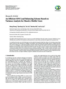
Cloud-oriented content delivery networks (CCDNs) is a gigantic distributed servers that delivers content to the individuals placed on geographical location of the user as shown in Fig. 1. [1]. This is due to the rapid increase of the user’s demand, the prime goal of the CCDNs to provide the web content to the end-users with significant level of availability and significant level of performance [2, 3]. For the large distributed system setting, requests reach from different users in an odd fashion. The main objective of any content provider is to search an efficient edge server at user’s doorstep [4, 5]. Voronoi diagram with Delaunay triangulation can decompose the earth surface in a nearest neighbor fashion. Therefore we have used Voronoi diagram

Fig. 1. Edge servers placed over geographical location II.

BACKGROUND STUDY

A. Voronoi Diagram in CDNs Definition 1: Let us assume P = {P1, P2, P3… Pn}, set of coordinate points as a location of edge servers. The Voronoi cell V(Pi) for Pi is defined as follows:

V ( Pi ) = { k : dist ( Pi , k ) < dist ( P j , k ) ∀ j ≠ i}

(1)

Voronoi diagram logically decompose the surface into a number of V(Pi) [8]. The V(Pi) for Pi, to be the set of coordinate point’s k over the plane which is closer to Pi than to any other point.

Fig. 2 describes the decomposition of earth surface into a number of Voronoi cell and also demarcates edge servers over the earth surface.

Fig. 2. An example of Voronoi diagram B. Delaunay triangulation over Voronoi diagram in CDNs Definition 2: For a considered set of coordinates P over the earth surface, Delaunay triangulation is defined such as no point of above mentioned set P repose inner side of the circumcircle of any triangle in the triangulation [9].

All load balancing algorithms are governed by four policies are discussed here. i) Load information among all nodes is keeping up-to-date, ii) transfer policy distributes with the different load information of the servers and based upon these information, servers may be as sender (transfer task to the edge server) or receiver mode (get task from another edge server). iii) Location policy deals with the geographical location of the edge server from user’s current location and iv) Selection policy is taken to choose which of the task is to be moved to the receiver ends. Determining load information of different edge servers are assigned at the beginning of execution using static load balancing technique, whereas dynamic load balancing algorithm is used to determine runtime information of load distributed among the edge servers [10]. Our FLRT load dynamic balancing algorithm is a load balancing strategy that approaches to update load information of the edge servers periodically and store in the database which is handled by any content provider. Our proposed algorithm initializes the databases with updated load information and meanwhile updated data used to be synchronized with time. Therefore keeping updated with last updated load information is one of the prime objective of our proposed algorithm. Different static and dynamic load balancing algorithms are discussed by many authors [11, 12, 17, 18, 19, 20, 21, 22]. III. PROPOSED ALGORITHM FOR SELECTION EFFICIENT EDGE SERVER

A. Our Fuzzy Based Dynamic Load Balancing Methodology Our dynamic load balancing method is developed by MatlabR2012b [13, 14]. Here we have categorized load index into five classes in between 0 to 1 and value of threshold is 0.5. Five Fuzzy sets are taken to depict the value of load index: very lightly load, lightly load, moderate load, heavy load and very heavy load as shown in Fig. 4.

Fig. 3. An example of Delaunay triangulation C. Load Balancing in CCDNs It is a mechanism for distributing task among different computers, CPUs or many devices. Primary objective of load balancing is to get maximum throughput, least response time and optimum resource utilization. It’s depends upon the load index which is usually notice a load imbalance state. This state in CCDNs means when the index at edge server is greater or smaller than the intended index value.

Fig. 4. Fuzzy index load chart For simulating our algorithm we have taken different value of load index (l) and threshold, therefore it can be changed depending on network situation [15, 16].

TABLE I.

FUZZY LOAD INDEX CHART BASED ON SERVER LOAD

1

μ verylightl yload (l ) =

0 .2 − l 0 .2 − 0 .1 0 0

μ lightlyloa d (l ) =

l < 0 .1 , l > 0 .5

1

0.2 < l < 0.4

0. 5 − l 0 .5 − 0 .4

0 .4 ≤ l ≤ 0 .5

l − 0 .4 0 .5 − 0 .4 0 .6 − l 0 .6 − 0 . 5

l < 0 .4 , l > 0 .6 0 . 4 ≤ l < 0. 5 0 .5 ≤ l ≤ 0 .6

l < 0 .5 , l > 0 .9

l − 0 .5 0 .6 − 0 . 5

0 .5 ≤ l ≤ 0 .6

1

0 .6 < l < 0 .8

0 .9 − l 0 .9 − 0 . 8

0. 8 ≤ l ≤ 0 . 9

0

μveryheavyload (l ) =

l > 0 .2

0.1 ≤ l ≤ 0.2

0

μ heavyload (l ) =

0.1 ≤ l ≤ 0.2

l − 0 .1 0 .2 − 0 .1

0

μmodearateload(l ) =

l < 0 .1

l − 08 0 .9 − 0 . 8 1

l < 0 .8 0 .8 ≤ l ≤ 0 .9 l > 0 .9

Assuming content service provider initiated the balancing algorithm, the proposed knowledge base is described below: Rule i: If (neighbor_edgeserver_load is verylightlyload) then (status_of_edgeserver is receiver) Rule ii: If (neighbor_edgeserver_load is lightlyload) then (status_of_edgeserver is receiver) Rule iii: If (neighbor_edgeserver_load is moderateload) then (status_of_edgeserver is receiver) Rule iv: If (neighbor_edgeserver_load is heavyload) then (status_of_edgeserver is sender)

Rule v: If (neighbor_edgeserver_load is veryheavyload) then (status_of_edgeserver is sender) Rule vi: If (status_of_edgeserver is sender) then select an active receiver from nearest neighbor edge server of the user’s location Rule vii: If the content service provider fails to find an active receiver and wait for next ‘ping’ time out time then (status_of_edgeserver is neutral) Our fuzzy sets output are shown in the following figure:

Fig. 5. Our proposed fuzzy output B. Our Proposed Algorithm for Efficient Edge Server Selection using Voronoi Diagram 1. Set lat = {lat1, lat2, lat3, …, latM} of latitudes of considered edge servers are stored in [1 × M] array 2. Set lon = {lon1, lon2, lon3, …, lonM} of longitudes of considered edge servers are stored in [1 × M] array 3. Set latv = {lat1, lat2, lat3, …, latM} of latitudes are stored in [M × 1] variable array 4. Set lonv = {lon1, lon2, lon3, …, lonM} of longitudes are stored in [M × 1] array 5. Set ip_addr = {ip_addr1, ip_addr2, …, ip_addrM} of IP addresses of considered edge servers are assigned in [1 × M] string array 6. Initially all the elements of visit array is 0 7. currentload Åcurrent load index value 8. for i Å 1 to size of lon 8.1 if lon(i) ≤ 0 then 8.2 lon(i) Å lon(i) + 360 // add 360° 8.3 end 9. end 10. voronoi(lon, lat) // Create a Voronoi diagram using the latitude and longitude value of edge servers 11. dt Å DelaunayTri(lonv, latv) // Create Delaunay triangulation over Voronoi diagram 12. my_lat Å22.56972 // Latitude of the current location 13. my_lon Å 88.36972 // Longitude of the current location 14. qrypt Å [my_lat my_lon] is a [ 1 × 2] array variable 15. [pid, Dist] ÅnearestNeighbor(dt, qrypt) // return pid and corresponding distance 16. if my_lon ≤ 0 16.1 my_lon Å my_lon + 360 17. end // add 360° 18. filenameÅ 'server_load_info.txt' // Load index from different edge servers 19. server_loadÅ importdata(filename)

20. load_index Åreadfis ('IndexLoad') 21. f Å readfis('IndexLoad.fis') 22. k Å 0 23. while(pid > 0 && pid 0) 23.4.1 [minavg I]Å min(data.avgres_time,[],1) 23.4.2 ip Å data.sltneighip (I, :) 23.4.3 pos Å data.ip_index (I) 23.4.4 if(pos == 0) 23.4.4.1 fprintf ('Request time out\n') 23.4.4.2 data.avgres_time(I) Å [] 23.4.4.3 data.sltneighip (I,:)Å [] 23.4.4.4 data.ip_index(I) Å [] 23.4.5 else if(visit(pos) ~= 1) 23.4.5.1 dos (['nslookup ' ip]) 23.4.5.2 data.avgres_time(I)Å []) 23.4.5.3 data.sltneighip (I,:) Å [] 23.4.5.4 data.ip_index(I) Å [] 23.4.5.5 visit(pos) Å 1 23.4.5.6 ruleview(f) 23.4.6 end 23.4.7 dim_dataavgrestime Å dim_dataavgrestime - 1 23.5 end

23.6 k Å k + 1 23.7 if (rem(k,2) == 1) 23.7.1 pid Å pid + k 23.7.2 rightpid Å pid 23.8 else 23.8.1 pid Å pid – k 23.8.2 leftpid Å pid 23.9 end 23.10 clear ans 24.11clear data 24. end 25. if (leftpid == 0) 25.1 pid Å rightpid + 1 25.2 while(pid ≤ size(dt)) 25.2.1 Step 23.1 To 23.5 25.3 pid Å pid + 1 25.4 clear ans 25.5 clear data 25.6 end 26. end 27. if (rightpid == size(dt) + 1) 27.1 pid = leftpid 27.2 while(pid > 0) 27.2.1 Step 23.1 To 23.5 27.3 pid = pid – 1 27.4 clear ans 27.5 clear data 27.6 end 28. end C. Simulation Analysis of Proposed Fuzzy Based Dynamic Load Balancing Method Step 1. Latitude and Longitude values of different edge servers are assigned in array variables (lat and lon) respectively that are listed in Table II and negative value of longitude are converted after adding 360° which are recorded in Table III. Step 2. IP addresses of different servers are stored in array variable named ip_addr and IP address with domain name and load of edge servers are collected in Table IV. Step 3. Partitioning different edge servers Voronoi diagram which is depicted in Fig. 6.

using

Step 4. Fig. 7 depicts Delaunay triangulation over the Voronoi diagram using set of latitude and longitude of enlisted servers. Step 5. Nearest neighbors are generated from the current location of requested user depending upon the latitude and longitude value and dt two dimension array variable of Delaunay triangulation as shown in Table V. Step 6. Servers situated at Colombo, New Delhi and Kolkata are selected as nearest servers for sending requested content of underlying CCDNs. Let, Kolkata is the current location of requested user.

TABLE III.

Fig. 6. Decomposing edge server using Voronoi diagram Step 7. Calculating accurate network latency time using ‘ping’ command over the nearest edge servers i.e. Kolkata, New Delhi and Colombo respectively which is recorded in Table VI. Step 8. Content service provider is selected an edge server based on minimum network latency time i.e. 56 ms. Step 9. Checking the load of the aforesaid edge server and our knowledge based fuzzy rule is applied on the selected edge server. Step 10. Rule i, ii & iii signify that the selected edge server is in receive mode for executing user’s request and Rule iv, v & vi mean that the selected edge server is sender mode. Step 11. Here servers located at Colombo, Kolkata and New Delhi are sender mode so that increase the pid value from user current pid value (i.e. 7). Now edge servers located at Islamabad, New Delhi and Colombo is selected for the pid value 8 which is also enlisted in Table VI. Selected edge servers located at Islamabad is now in receiver mode to serve user’s request. Otherwise our proposed algorithm selects the pid values 6, 8, 5, 9, 4, 10, 3, 11, 2, 12, 1, 13, 14 and so on. Our objective is to select pid value one by one after increasing or decreasing from the current pid value which is explained in the pseudocode (line number 23 - 28). TABLE II.

LIST OF CONSIDERED EDGE SERVERS

Edge Server Ankara Buenos Aires Canberra Cape Town Chicago Colombo Harare Islamabad Kingston Kolkata London Mexico New Delhi Santiago Singapore

Latitude 39.93°N 34.6033°S 35.3075°S 33.9253°S 41.8819°N 6.9345°N 17.8639°S 33.7166°N 44.2333°N 22.5666°N 51.5073°N 19.000°N 28.6138°N 33.4500°S 1.3°N

Longitude 32.87°E 58.3818°W 149.1243°E 18.4238°E 87.6277°W 79.8429°E 31.0298°E 73.0666°E 75.6918°W 88.3666°E 0.1275°W 99.1333°W 77.2089°E 70.6667°W 103.9°E

LATITUDE, LONGITUDE AND MODIFIED LONGITUDE OF EDGE SERVERS

Edge Servers Ankara Buenos Aires Canberra Cape Town Chicago Colombo Harare Islamabad Kingston Kolkata London Mexico New Delhi Santiago Singapore

Latitude 39.93 -34.6033 -35.3075 -33.9253 41.8818 6.9345 -17.8639 33.7166 44.2333 22.5666 51.5073 19.0000 28.6138 -33.45 1.3

Longitude 32.87 -58.3818 149.1243 -18.4238 -87.6277 79.8429 31.0298 73.0666 -75.6918 88.3666 -0.1275 -99.1333 77.2088 -70.6667 103.9

Modified Longitude 32.87 301.6182 149.1243 341.5762 272.3723 79.8429 31.0298 73.0666 284.3082 88.3666 359.8725 260.8667 77.2088 289.3333 103.9

Fig. 7. Delaunay triangulation with Voronoi diagram TABLE IV.

IP ADDRESS WITH DOMAIN NAME OF EDGE SERVERS

Location

IP Address

Domain Name

Ankara

159.253.37.36

Buenos Aires Canberra

157.92.5.71

ankarauni.esntu rkey.org www.uba.ar

Cape Town Chicago Colombo Harare

192.148.223.248

Current load 0.60 0.50 0.30

137.158.158.44

www.acu.edu.a u www.uct.ac.za

128.248.155.15 220.247.217.154 209.88.91.222

www.uic.edu www.ibmbb.lk www.hit.ac.zw

0.20 0.85 0.0

61.5.158.124

www.islamabad airport.com.pk kingstonuniversity.us www.becs.ac.i n www.lon.ac.uk

0.40

Islamaba d Kingston

66.96.146.129

Kolkata

14.139.223.176

London

128.86.130.195

Mexico New Delhi Santiago Singapore

64.106.44.210 113.30.141.196 158.170.64.116 155.69.254.5

www.unm.edu www.imsghaziabad.ac.in www.usach.cl www.ntu.edu.s g

0.10

0.20 0.80 0.1 0.1 0.80 0.35 0.70

TABLE V. pid value 1 2 3 4 5 6 7 8 9 10 11 12 13 14 15 16 17 18 19 20 21 22

Neighbor I

TABLE VI. Location of Edge Servers Kolkata New Delhi Colombo Islamabad Colombo New Delhi

REFERENCES

DT VALUES OF DELAUNAY TRIANGULATION

8 6 7 10 10 10 10 8 12 12 7 5 9 9 14 11 3 15 9 9 14 9

Neighbor II 1 7 6 6 8 5 13 6 10 5 5 1 5 1 2 1 14 3 12 2 3 4

Neighbor III 6 15 1 15 13 8 6 13 15 10 15 8 12 5 12 9 12 12 2 4 2 11

OUR PROPOSED KNOWLEDGE BASED OUTPUT Average Our Fuzzy Least Output Response Time pid value = 7 181 ms 0.8147 56 ms 0.8147 Request time 0.8089 out pid value = 8 227 ms 0.1853 Request time 0.8089 out 56 ms 0.8147

Our Proposed Knowledge Based Output Sender Sender Sender

[1]

[2]

[3]

[4]

[5]

[6] [7]

[8]

[9] [10]

[11]

[12]

[13] Receiver Previously deselect Previously deselect

IV. CONCLUSION AND FUTURE WORKS Our proposed algorithm and simulation results promulgate minimum network latency, server load and packet loss for selecting efficient edge server over the earth surface. In this manuscript we have used Voronoi diagram to decompose the earth surface. Subsequently we have also applied Delaunay triangle for finding nearest edge server from user’s current location. In this paper, our fuzzy based dynamic load balancing algorithm (FLRT) can make absolute outputs for inconstancy inputs. Our vigorous algorithm is fit for upcoming internet trends. We are applied our dynamic load balancing strategy on fifteen different servers which are scattered over large geographical region over the earth surface. In near future we will try to implement our FLRT dynamic load balancing algorithm in real environment. Moreover we will use our aforementioned balancing paradigm in parallel and distributed systems to observe whether our method will be smarter than previous application or not.

[14]

[15]

[16]

[17]

[18] [19] [20] [21] [22]

C. Papagianni, A. Leivadeas, and S. Papavassiliou, “A CloudOriented Content Delivery Network Paradigm: Modeling and Assessment,” Dependable and Secure Computing, IEEE Transactions, vol. 10, no. 5, pp. 287-300, 2013. M. Pathan, R. Buyya, and A. Vakali, “Content Delivery Networks: State of the Art, Insights, and Imperatives,” CDNs, vol. 9, no. 1, pp. 3-32, 2008. J. Broberg, R. Buyya, and Z. Tari, “MetaCDN: Harnessing ‘Storage Clouds’ for high performance content delivery,” J. Net. and Comp. App., vol. 32, no. 5, pp. 1012-1022, 2009. M. Afergan, A. LaMeyer, and J. Wein, “Experience with some principles for building an internet-scale reliable system. In proc. 2nd USENIX Workshop on Real, Large Distributed Systems, Worlds, USA, December 2005. F. Douglis, A. Feldmann, B. Krishnamurthy, “Rate of Change and other Metrics a Live Study of the World Wide Web,” USENIX Symposium on Internetworking Technologies and Systems, December 1997. R. Klein, “Concrete and Abstract Voronoi Diagrams,” LNCS, Springer-Verlag Berlin Heidelberg, vol. 400, no. 1, pp. 169, 1989. F. Aurenhammer, “Voronoi Diagrams—A Survey of a Fundamental Geometric Data Structure,” ACM Computing Surveys, vol. 23, no. 3, pp. 345–405, September 1991. K. Mehlhorm, S. Meiser, and C. O’Dunlaing, “On the Construction of Abstract Voronoi Diagrams,” Discrete & Computational Geometry, Springer-Verlag New York Inc. vol. 6, pp. 221-224, 1991. F. Aurenhammer, R-D Klein, and D-T Lee, “Voronoi Diagrams and Delaunay Triangulations,” World Scientific, 2013 S. Sharma, S. Singh, and M. Sharma, “Performance Analysis of Load Balancing Algorithms,” World Academy of Science, Engineering and Technology 38, 2008, pp. 269-272. Y. T. Wang, and R. J. T., “Morris, Load Sharing in Distributed Systems,” IEEE Transactions on Computers, vol. 34, 1985, pp. 204217. W. Leinberger, G. Karypis, V. Kumar and R. Biswas, “Load Balancing Across Near-Homogeneous Multi-Resource Servers,” In 9th Heterogeneous Computing Workshop, Cancun, Mexico, 2000.D. D. Sarddar, S. Roy and R. Bose, “An Efficient Edge Servers Selection in Content Delivery Network Using Voronoi Diagram,” IJRITCC, vol. 2, no. 8, pp. 2326 – 2330. S. Roy, R. Bose, D. Sarddar, “A Novel Replica Placement Strategy using Binary Item-To-Item Collaborative Filtering for Efficient Voronoi-Based Cloud-Oriented Content Delivery Network,” in Proceeding International Conference on Advances in Computer Engineering and Applications-2015, 19-20th March, Ghaziabad, India. M. Livny, and M. Melman, “Load balancing in homogeneous broadcast distributed systems,” In Proc. ACM Computer Network Performance Symposium, 1982, pp. 47-55. A. Karimi, F. Zarafshan, A. b. Jantan, A. R. Ramli, and M. I. b. Saripan, “A New Fuzzy Approach for Dynamic Load Balancing Algorithm,” IJCSIS, vol. 6, no. 1, 2009. H. Singh, Dr. S. Kumar, “Dispatcher Based Dynamic Load Balancing on Web Server System,” IJGDC, vol. 4, no. 3, September 2011, pp. 89-106. R. Motwani, and P. Raghavan, “Randomized algorithms,” ACM Comp. Surv., vol. 28, no. 1, 1996, pp. 33-37. Z. Xu, R. Huang, "Performance Study of Load Balancing Algorithms in Distributed Web Server Systems,” CS213 Project Report. T. H. Cormen, C. E. Leiserson, R. L. Rivest, and C. Stein, “Introduction to Algorithms,” MIT Press, 2nd Edition, 2001. J. A. Hartigan, “Clustering Algorithms,” John Wiley & Sons, New York, 1975. P. L. McEntire, J. G. O’Reilly, R. E. Larson, “Distributed Computing: Concepts and Implementations”, IEEE Press, 1984.