2011 19th International Euromicro Conference on Parallel, Distributed and Network-Based Processing
Dynamic Load Balancing for High-Performance Simulations of Combustion in Engine Applications Laura Antonelli and Pasqua D’Ambra Institute for High Performance Computing and Networking Italian National Research Council Naples, Italy Email: laura.antonelli,
[email protected] cells have low probability to be assigned to the same processor. In the case of homogeneous computing architectures, per each distribution strategy, the dimension of the subgrid assigned to the single processor is the same per each processor, while to get performance in the use of heterogeneous platforms, the dimensions of the local subgrids take into account the performance of the different CPUs. In all the cases, the data partitioning is static, i.e. it does not change during the simulation, except when changes in the global grid happen. Numerical results on our test cases show that the random distribution is a good choice to balance workload among the processors and hence to obtain good parallel efficiency. For details on the algorithms and on the results we refer the reader to [3], [4], [5]. However, since in the cyclic and random distributions contiguous cells are generally assigned to different processors, they are not appropriate when the combustion task is part of a multicomponent code for engine simulations, in which solvers for the Partial Differential Equations (PDEs) driving the fluid flow require frequent interactions among contiguous grid cells. In this case, grid partitioning employing blocks of contiguous cells are desirable, indeed it minimizes the so-called surfaceto-volume effect [8] and requires data exchanges only among neighbor processors. Here, we discuss first results related to the use of a dynamic load balancing algorithm, in which non-uniform blocks of contiguous grid cells are assigned to contiguous processors, logically connected as in an acyclic ring, and dimension of the blocks is periodically changed according with a measure of their computational workload, varying along the simulation. In this way, boundaries of local subgrids are locally changed at each new partitioning, but pattern and volume of the needed data exchanges within possible coupled parallel PDE solvers remain unchanged. The paper is organized as following: in Section II we introduce main features of our combustion parallel solver, both in terms of ODE solvers and in terms of parallelism. In Section III we describe the strategy of dynamic load balancing algorithm for data partitioning. In section IV we introduce the benchmark of our engine test cases and on these test we analyze in Section V performance of combustion parallel solver with pure block distribution as well as the workload imbalancing. In Section VI we discuss preliminary results obtained with dynamic distribution and we compare this with pure block distribution on our test cases. Finally, in Section VII we report some concluding remarks.
Abstract—The chemical task in internal combustion engine simulations concerns with the solution of a non-linear stiff system of Ordinary Differential Equations (ODEs) per each cell of a discretization grid representing engine geometry. The computational cost of the above task, when a detailed kinetic scheme is used, is dominating in engine simulations. Due to local physicalchemical conditions, each system of ODEs is characterized by local numerical properties (such as stiffness), therefore local adaptive solvers are usually employed for its efficient solution. We developed an MPI-based combustion parallel solver for efficient solution of the chemical task in engine simulations within parallel environment. In this context, we propose a cell distribution based on a dynamic load balancing algorithm, using a strategy which preserves contiguousness of the computational grid cells. Efficiency of our approach is shown for parallel simulations of realistic Diesel engines, when different sizes of the discretization grid and different operative conditions of the engine are used. Keywords-parallel combustion simulation; dynamic load balancing; data partitioning.
I. I NTRODUCTION Reducing air pollutant emissions for matching the stringent limits imposed by the Governments led engine designer to adopt multidimensional simulation codes, involving detailed kinetics reaction mechanisms for well understanding of combustion development and pollutants formation. In this context, we proposed a combustion parallel software component in order to make efficient and scalable simulations of realistic engines. Our software component is based on an adaptive multisolver for effective solution of the local stiff ODE system at each grid cell of the computational domain, and it employs different strategies of grid cell partitioning for reducing load imbalance due to local numerical features. Data partitioning and load balancing are key issues in parallel computation and many different partitioning strategies have been proposed and successfully applied within scientific codes [15], [7]. In our combustion simulation code, since the reaction operator does not introduce coupling among the grid cells, data partitioning does not influence communication among the processors during the computation, but only computational load balancing because of the different computational workload associated to different grid cells. The combustion software supports the usual pure block partitioning, where a block of contiguous cells is distributed to each processor. Furthermore, cyclic and random partitioning are also employed. In these two cases, cells are scattered among the processors in a way that near 1066-6192/11 $26.00 © 2011 IEEE DOI 10.1109/PDP.2011.88
133
II. PARALLEL A DAPTIVE S OLVER FOR E NGINE C OMBUSTION
However, since numerical features of system (1) are strongly related to local physical/chemical conditions of the fluid flow, when adaptive solvers are considered in a parallel environment, data partitioning becomes the key issue for computational load balancing and for reduction of processor idle times. In the last years [3], [4], [5], we proposed a combustion parallel software component to be used in simulation of Diesel engine combustion, when detailed chemistry is considered. The software component is written in Fortran 77 and it uses MPI [14] for process management and data communication. It is based on CHEMKIN-II [12] for setting model parameters involved in system (1) within a Fortran simulation code. Our combustion component has been interfaced with the sequential KIVA3V-II code [2], in order to properly test it within real simulations. The KIVA family of codes has been developed since ’80 years at Los Alamos National Laboratories and its modifications are being used worldwide for engine applications. However, the various versions of the code include reduced chemical reaction mechanisms for combustion modeling and numerical algorithms that are inadequate for coupled solution of detailed mechanisms. For our aim, we substituted the original KIVA combustion submodel with our combustion software. It selects for each grid cell of the overall 3D domain a suitable ODE integration algorithm. Each algorithm chosen for one grid cell may differ from the others both for integration method and for time substeps employed during the integration. Note that the physical features of the Diesel combustion implies that neighboring cells have similar chemical-physical conditions and then similar numerical properties. Therefore grid cells with high computational complexity are close. In this framework, the partitioning of the computational domain is a critical issue for load balancing. Our combustion parallel software supports three different static grid partitioning strategies, in order to use the best strategy depending on the chemistry model, the computational grid and the computing platform at the hand. The three strategy are named pure block, cyclic and random distributions. The pure block distribution is the usual partitioning where a block of contiguous grid cells is assigned to each processor. In the cyclic distribution grid cells are scattered among the processors according to a round-robin circular algorithm; in this way contiguous cells are assigned to different processors in order to avoid that cells with high computational cost are assigned to the same processor. In random distribution before applying pure block distribution, grid cells indeces are ordered according with a pseudo-random sequence. Since pseudo-random scattering is realized, the probability to assign contiguous cells to the same processor is reduced. In all the three distributions the processors are disposed in a virtual geometry like an acyclic ring. In the case of homogeneous platforms, the dimension of the subgrids assigned to each processor is the same and it does not change during the simulation, except when the overall grid changes during the simulation, as in the case of the KIVA code. Although the experimental results on our test cases show that the random distribution is the most efficient strategy for reducing load imbalance in the solution of the combustion submodel, it is not an appropriate choice when the combustion
Mathematical models for simulations of internal combustion engines usually involve unsteady Navier-Stokes equations for turbulent multicomponent mixtures of gases, coupled with model for describing phenomena such as fuel spray, evaporation and combustion. Operator splitting is typically used for numerical solution of the overall model, where different physical/chemical phenomena are decoupled and different submodels are solved independently, at each time-splitting interval. One of the main computational kernels in this framework is the solution of the combustion submodel, especially when detailed kinetics models are considered. It describes chemical reactions involving a high number of chemical species, characterized by very different reaction rates. The non-linear ODE system, describing the rate of change of the chemical species concentration due to reactions, has the following form: ρ˙ m = Wm
R !
(bmr − amr ) ω˙ r (ρ1 , . . . , ρM , T ) ,
r=1
(1)
m = 1, . . . , M
where M is the number of chemical species, R is the number of chemical reactions, ρ˙ m is the production rate of species m, Wm is its molecular weight, amr and bmr are integral stoichiometric coefficients for reaction r, ω˙ r is the kinetic reaction rate and T is the temperature. This system, coming from the mass balance equations for the different species involved in the combustion process, is characterized by a high degree of stiffness due to the strongly different reaction rates of the species, and its solution is required per each grid cell of the overall discretization grid, representing the engine geometry. During a Diesel combustion process, the mathematical features of system (1) change, since two main combustion phases can be identified. The low temperature phase or autoignition is the period from the start of fuel injection to ignition and it is characterized by a high degree of stiffness. The high temperature phase or combustion from ignition onwards is instead characterized by a smoother kinetic dynamics, and a lot of intermediate species are rapidly damped. Therefore, reliable solution of (1) for the overall combustion process simulation has been obtained by means the local adaptive multisolver described in [3]. The solver is based on a suitable merge of two implicit methods, each one of them operates on a different combustion phase: variable coefficient Backward Differentiation Formulas [9] are employed in the autoignition phase and a 5-stages Singly Diagonally Implicit Runge-Kutta (SDIRK) method [11] is used in the combustion phase. These methods are available in two different open-source software packages, namely VODE [6] and SDIRK4 [11], respectively. As already observed in Section I, the right-hand side of system (1) does not introduce spatial coupling among the grid cells, therefore, the solution of the combustion submodel involved in engine simulations is well suited to take advantage from parallelism. As a matter of fact engine combustion is a typical problem where parallel and distributed computing are used to exploit both detailed chemical schemes and efficient solutions (you can see [1], [3], [13]).
134
dimension. Of course, the new partition is generally nonuniform and induces a nonuniform block grid partitioning among the concurrent # " processors. Let P old := Ipold p=1,...,P be a partition of the set I, associated to the computational grid cells of a combustion parallel simulation on P processors, and suppose that processor p, at the current time-splitting interval s, owns the grid cells in Ipold . At the end of the simulation on interval s, dynamic algorithm evaluates a measure of the total computational load imbalance, as: Ts − Ts (2) Rs = max s med , Tmax $P T old p=1 p s s where Tmax = max Tpold , Tmed = and Tpold P
task is part of a multicomponent code for engine simulations. Indeed, solvers for the PDEs driving the fluid flow require interactions among contiguous grid cells, therefore grid partitioning employing assignment of blocks of contiguous cells to contiguous processors are desirable since it realizes the socalled surface-to-volume effect. Indeed, in the case of blocks of contiguous cells representing a subdomain of the overall computational domain, the communication requirements of a processor are proportional to the surface of the subdomain assigned to the processor, while the computational cost is proportional to the subdomain volume. Therefore, the communication to computation ratio decreases as the subdomain size increases. Our focus in this work is to show the improvement in efficiency as well as in reducing of load imbalancing when a strategy of workload dynamic distribution is applied in our combustion parallel software with pure block partitioning.
p=1,...,P
is the workload of processor p at the simulated time-splitting interval s, i.e.: ! Tpold = T s (i) . i∈Ipold
III. DYNAMIC L OAD BALANCING A LGORITHM
The dynamic algorithm assumes that the workload of parallel computation was imbalanced among the processor on interval s, if: Rs > r with 0 < r < 1 , (3)
Dynamic load balancing is one of the key techniques exploited to improve the performance of parallel algorithms [15], [7]. Usually this technique is based on transferring units of computational work (part of the total workload) among processors at run time to maintain global load balance. The measure of the workload often depends on specific application and algorithm. For estimating at run time a possible load imbalance in our combustion parallel solver, we defined a workload measure, taking into account that the main source of load imbalance is due to different computational cost needed to solve system (1) at different grid cells and time intervals. Let P be the number of concurrent processors, numbered from 1 to P , and N the total number of grid cells with indices in the set I = {1, 2, . . . , N }. Suppose that, at a current timesplitting interval s, of an engine simulation, processor p owns a subgrid of dimension Np , corresponding to a subset Ip ⊂ I, where P := {Ip }p=1,...,P is a partition of I. We assume as processor workload measure on current time-splitting interval s, the total computational time Tps spent by the processor p in the solution of system (1) on its subgrid Ip : ! Tps = T s (i) ,
where r is a suitable input threshold fixed by the user as the maximum rate of acceptable load imbalance. When the condition (3) is true, the algorithm advances to define a new partition of the set I for the next interval s + 1, as: " # P new := Ipnew p=1,...,P , (4)
where Ipnew is a set of contiguous cell indices for which the corresponding total workload, estimated as: ! Tpnew = T s (i) (5) i∈Ipnew
s is as close as possible to Tmed . In other words, starting from new the first indices set I = {1, . . . , N1new }, such that T1new = 1 $ s s i∈I1new T (i) ≤ Tmed , each new index subset is obtained as the subset: " new # new Ipnew = Np−1 + 1, Np−1 + 2, . . . , Npnew , p = 2, . . . , P
i∈Ip
such that:
s
where T (i) is the so-called computational workload unit, i.e. the computational time that processor p spends to solve system (1) on i-th cell at the current time-splitting interval s. As explained in Section II, our code uses an adaptive solver for solving system (1) at each time-splitting interval, using different time steps and possibly different formulas, independently at each grid cell. Therefore, at each time-splitting interval s, the values of Tps can be very different among the processors, leading to a computational load imbalance which can seriously affects the parallel performance of the code. In order to reduce the difference between processors workload measured by Tps values, the key idea of the dynamic load balancing algorithm is to define a new partition P new before starting a new time-splitting interval, where each subset Ip , made of a block of contiguous indices, has a suitably computed
Tpnew =
!
T s (i)
≤
s Tmed
.
i∈Ipnew
If after the above partitioning, the total set I is not exhausted, the remaining indices are assigned to the processor P, in order to preserve the index contiguousness in each subset Ipnew . This is a reasonable choice, because the way we obtain the partition P new produces a (possible) very small number of remaining cells. The new partition is applied before starting the combustion parallel solver on the next time-splitting interval s + 1. If the condition (3) is false, the old grid partition P old is used on interval s + 1. Starting the parallel simulation at the first time-splitting interval, by using a pure block grid partitioning, where the dimension of the all subsets Ip is
135
TABLE II T OTAL E XECUTION T IMES ( SEC .) OF PARALLEL C OMBUSTION S OLVER : Pure Block Distribution VS Dynamic Distribution
TABLE I O PERATING C ONDITIONS OF T EST C ASES
Test Case Case 1 Case 2 Case 3
RP [bar] 500 900 500
EGR [crank] 40% 0% 0%
IC [crank] 12.7 2.3 2.1
IP [crank] 7.3 5.7 7.3
Np = N/P 1 , the above dynamic strategy is used to define a possible new grid partition from an old one, at each timesplitting interval. Note that the application of the dynamic load balancing algorithm only requires two global reductions for obtaining the measure of the total load imbalance in (2), therefore, the cost of the algorithm in terms of data communication is negligibile as the extra computational work required at each time-splitting per each processor for obtaining the new partition P new from the old one P old . IV. BACKGROUND
AND
D ETAILS OF THE S IMULATIONS
P 1 2 4 8 16 32 64
Case 1 55518 29106 16960 8618 4581 2341 1354
P 2 4 8 16 32 64
Case 1 28935 15361 7700 3908 1996 1065
Pure Block Distribution small grid large grid Case 2 Case 3 Case 1 Case 2 Case 3 52090 48922 70015 84850 107714 27319 29131 37268 43069 60282 14119 14908 22420 24575 34304 7051 7498 12171 12697 21648 3860 3994 6532 6487 13321 2278 2235 3795 3607 9235 1503 1281 1963 1930 7398 Dynamic Distribution small grid large grid Case 2 Case 3 Case 1 Case 2 Case 3 27481 25125 36081 44101 56505 14798 13501 19520 23114 32620 7970 6851 9679 11736 17980 4108 3404 5488 5995 11325 2391 1724 2814 2944 8229 1483 865 1571 1566 6786
TABLE III R ISE FACTOR OF ODE SOLVERS COUNTERS GOING FROM small grid TO large grid
Our benchmark is a realistic engine describing a prototype of a single cylinder Diesel engine. The detailed chemical model used in our simulation is a modification of the scheme introduced in [10], composed of N-dodecane as primary fuel and involves 62 chemical species and 285 reactions. Our typical computational grid is a 3D cylindrical sector representing a sector of the engine cylinder and piston-bowl. We consider two geometrical grids, characterized by two different total number of cells: about 2519 cells for the so-called small grid and about 4571 cells for the so-called large grid. The cells are numbered in counter-clockwise fashion on each horizontal layer, from bottom-up. Note that, the structure and the dimension of the grid on which the combustion parallel solver runs change during a simulation of the entire engine cycle, as managed by the KIVA3V-II code to follow the piston movement into the cylinder. The limit positions of the piston, that is the lowest point from which it can leave and the highest point it can reach, are expressed with respect to the so-called Crank angle values and they correspond to −180o and 0o . During the typical interval of the Crank angles ([IC, 40o ]), in which main combustion phenomena happen, the total number of active cells according to piston movement, varies between 945 and 1080 for small grid and between 945 and 1755 for large grid. Our prototype engine operates at three different conditions, which corresponds to three different test cases named Case 1, Case 2 and Case 3. Details on operating conditions are summarized in Table I, where RP is the rail pressure, EGR is the Exhaust Gas Recirculation, IC is the Crank angle in which fuel injection starts and IP is the injection timing. The experiments were carried out on a HP XC 6000 Linux cluster with 64 bi-processor nodes, operated by the Naples branch of ICAR-CNR. Each node comprises an Intel Itanium 2 Madison processor, with clock frequency of 1.4 Ghz, and is equipped with 4 GB of RAM; it runs HP Linux for High Performance Computing 3 (kernel 2.4.21). The main
nstep nfe nje nlu
Case 1 1.66 2.70 1.62 1.67
Rise Factor Case 2 Case 3 1.75 2.19 1.42 1.66 1.61 2.23 1.55 1.93
interconnection network is Quadrics QsNetII Elan 4, which has a sustained bandwidth of 900 MB/sec and a latency of about 5 µsec for large messages. The GNU Compiler Collection, v. 4.2, and the HP MPI implementation, v. 2.01, have been used. For the results we discuss here, we used a number of processors ranging from 1 to 64. In the upper part of Table II we show the total execution times of the parallel combustion solver within a simulation of the Carnk angle interval [IC, 40o ], when a static and uniform pure block grid distribution is used on the three test cases, per each available grid. All the times are measured by calling MPI timing routines in the code, before and after calling the combustion solver at each time-splitting interval, and accumulating the time during the overall simulation. We note that for the small grid the three test cases led to generally comparable execution times, while changing the grid, Case 3 shows a large increase in the time spent in the combustion solver. In order to analyze this increasing in going from small to large grid, in Table III we show the rise factors of the following counters, accounting for the computational cost of general implicit ODE solvers for solving system (1): • • • •
1 If N is not a multiple of P , the first n subsets have dimension N + 1, p where n = mod(N, P ).
nstep, number of time integration substeps; nfe, number of function evaluations; nje, number of Jacobian evaluations; nlu, number of LU factorizations;
We can see that for Case 1 and Case 2 the rise factors for 136
Fig. 1. Speed-up of Parallel Combustion Solver on small grid: Pure Block Distribution vs Dynamic Distribution
Fig. 3. Speed-up of Parallel Combustion Solver on large grid: Pure Block Distribution vs Dynamic Distribution
64
64 Block Case 1 Block Case 2 Block Case 3 Dynamic Case 1 Dynamic Case 2 Dynamic Case 3
Speedup
Speedup
Block Case 1 Block Case 2 Block Case 3 Dynamic Case 1 Dynamic Case 2 Dynamic Case 3
32
32
16
16
8
8
4 2
4 2 2 4
8
16
32 Number of Processors
64
2 4
Fig. 2. Efficiency of Parallel Combustion Solver on small grid: Pure Block Distribution vs Dynamic Distribution
8
16
32 Number of Processors
64
Fig. 4. Efficiency of Parallel Combustion Solver on large grid: Pure Block Distribution vs Dynamic Distribution
1
1 0.8
0.8
Efficiency
0.6
Efficiency
0.6 0.4
0.4 0.2
Block Case 1 Block Case 2 Block Case 3 Dynamic Case 1 Dynamic Case 2 Dynamic Case 3
0.2
Block Case 1 Block Case 2 Block Case 3 Dynamic Case 1 Dynamic Case 2 Dynamic Case 3
0 2 4
8
16
32
64
Number of Processors 0 2 4
8
16
32
64
Number of Processors
nstep, nje and nlu are comparable. However, while Case 1 shows the rise factor for nfe higher than the other two test cases, Case 3 presents the highest rise factors for the other counters. When the large grid is used on Case 3, the solution process based on Newton-type iterations converges at a slow rate, then in order to satisfy accuracy requests, the employed ODE solver requires many reductions of time substeps. This needs both the construction and the LU factorization of a new Jacobian matrix, which account for a large computational cost. On the other hand, the simulation of Case 1 on large grid forces the combustion solver to use a one-order formula (backward Euler) for a lot of grid cells in many time-splitting intervals in order to balance accuracy requests and computational cost, and this is the main reason of the large increase in the number of function evaluations. However, as expected, an increasing in function evaluations has a lower impact on the execution times with respect to the increasing of the other three counters. V. P ERFORMANCES AND M EASURES OF W ORLOAD P URE B LOCK D ISTRIBUTION
respectively, of the parallel software when the pure block distribution is applied on small grid. We can see that speedup and efficiency decrease when the number of processors increases. We can observe on 64 processors, a speed-up of about 44 for Case 1 and of about 41 for Case 3 which corresponds to a parallel efficiency of about 68% and 65%, respectively. A lower speed-up of about 37 is shown for Case 2 corresponding to a parallel efficiency of about 58%. In Fig. 3 and in Fig. 4 we report the speed-up and the efficiency, respectively, when the pure block distribution is applied on large grid. Except for Case 2, we can observe a more serious reduction of both speed-up and efficiency when the large grid is used for the different test cases, showing that the problem of an efficient combustion simulation is very sensitive to the engine operating conditions and grid sizes. In particular, very low speed-ups of about 13 and 16 were obtained for Case 3 on 32 and 64 processors, respectively, which corresponds to 39% and 25% of efficiency. Despite of a computational cost increasing of Case 3 on large grid, Case 2 shows the better performances with respect to small grid, achieving a speed-up of about 45 with an efficiency of about 69% on 64 processors. In order to deep inside the above performance behaviour, we measured the mean value, µ, and the standard deviation, σ, of
IN
In this Section we show the performances of the parallel combustion solver with pure block distribution in the simulations of the three test cases described in section IV. In Fig. 1 and in Fig. 2 we report the speed-up and the efficiency,
137
TABLE IV W ORKLOAD I MBALANCE M EASURES OF PARALLEL C OMBUSTION S OLVER : Pure Block Distribution VS Dynamic Distribution ON small grid
P 2 4 8 16 32 64
Case 1 µ (σ) 0.07 (0.04) 0.23 (0.09) 0.29 (0.10) 0.37 (0.11) 0.46 (0.14) 0.56 (0.15)
RG 0.04 0.18 0.19 0.24 0.26 0.36
P 2 4 8 16 32 64
Case 1 µ (σ) 0.06 (0.05) 0.14 (0.05) 0.20 (0.07) 0.26 (0.09) 0.34 (0.11) 0.44 (0.13)
RG 0.03 0.09 0.09 0.11 0.13 0.18
Pure Block Distribution Case 2 µ (σ) RG 0.07 (0.04) 0.05 0.20 (0.09) 0.08 0.31 (0.11) 0.07 0.41 (0.12) 0.16 0.49 (0.14) 0.28 0.60 (0.16) 0.46 Dynamic Distribution Case 2 µ (σ) RG 0.07 (0.05) 0.04 0.15 (0.07) 0.12 0.21 (0.10) 0.18 0.27 (0.11) 0.21 0.35 (0.13) 0.32 0.46 (0.15) 0.45
TABLE V W ORKLOAD I MBALANCE M EASURES OF PARALLEL C OMBUSTION S OLVER : Pure Block Distribution VS Dynamic Distribution ON large grid
Case 3 µ (σ) RG 0.14 (0.06) 0.16 0.28 (0.07) 0.18 0.37 (0.09) 0.18 0.45 (0.10) 0.23 0.54 (0.13) 0.31 0.63 (0.15) 0.40
P 2 4 8 16 32 64
Case 1 µ (σ) RG 0.09 (0.07) 0.06 0.27 (0.10) 0.22 0.37 (0.10) 0.28 0.46 (0.12) 0.33 0.58 (0.13) 0.42 0.67 (0.13) 0.44
Case 3 µ (σ) RG 0.05 (0.05) 0.02 0.15 (0.06) 0.09 0.20 (0.08) 0.10 0.27 (0.10) 0.10 0.36 (0.12) 0.11 0.47 (0.13) 0.11
P 2 4 8 16 32 64
Case 1 µ (σ) RG 0.05 (0.06) 0.02 0.17 (0.08) 0.09 0.26 (0.12) 0.09 0.35 (0.15) 0.20 0.46 (0.17) 0.22 0.56 (0.17) 0.30
the load imbalance measure during the simulations: % $S $S 2 R s s=1 (Rs − µ) µ = s=1 , σ= , S S
Pure Block Distribution Case 2 µ (σ) RG 0.07 (0.04) 0.01 0.23 (0.08) 0.13 0.33 (0.10) 0.16 0.41 (0.10) 0.18 0.51 (0.11) 0.26 0.62 (0.12) 0.31 Dynamic Distribution Case 2 µ (σ) RG 0.05 (0.04) 0.03 0.13 (0.05) 0.08 0.19 (0.07) 0.09 0.25 (0.11) 0.11 0.34 (0.13) 0.10 0.44 (0.15) 0.15
Case 3 µ (σ) RG 0.12 (0.07) 0.10 0.29 (0.09) 0.21 0.41 (0.10) 0.37 0.48 (0.12) 0.49 0.59 (0.14) 0.56 0.68 (0.15) 0.77 Case 3 µ (σ) RG 0.08 (0.08) 0.04 0.17 (0.12) 0.17 0.23 (0.14) 0.25 0.30 (0.16) 0.40 0.40 (0.18) 0.58 0.50 (0.19) 0.74
VI. DYNAMIC L OAD BALANCING V ERSUS P URE B LOCK D ISTRIBUTION (6)
In the following we analyze the performance of the parallel combustion solver when the dynamic load balancing algorithm is applied. We used a threshold r = 0.1 as maximum load imbalance allowed per each time-splitting interval. In the bottom part of Table II we show total execution time of the combustion parallel solver within a simulation, on the three test cases, per each available grid. Note that for P = 1 the data partitioning corresponds to pure block distribution and so these data are not shown in the bottom part of Table II. We can see a general reduction of the total execution time with respect to pure block distribution for both the available grids and for all the test cases except for Case 2 on small grid. Indeed for this simulation, we observe an unexpected increase of the execution times for all the number of processors, save for p = 64 processors where a slight decrease of the time is gained. more in details, we note for small grid that Case 1 and Case 3 show a reduction of the execution times for each number of processors. This reduction leads to an improvement of performances with respect to pure block distribution as it is evident in Fig. 1 and Fig. 2, where we show speed-up and efficiency of the parallel solver with dynamic distribution (vs pure block distribution) on small grid. We can observe a speedup of about 55 on 64 processors for Case 1 and of about 56 for Case 3, corresponding to a parallel efficiency of about 86% and 88%, respectively. The performance gains of the parallel solver come from the introduction of the dynamic strategy in block data partitioning that points on a partition of suitably dimensioned blocks of contiguous grid cells for reducing the workload imbalancing in our simulations. This goal is reached as it is inferred in the bottom part of Table IV, where we show both the measures (6) and (7) of workload imbalancing. In general, we note a reduction of imbalancing both ‘local” and “global” of the workload. In details, we note that we have obtained an
where S is the total number of time-splitting intervals in [IC, 40o ]. We also measured the following total load imbalance: Tmax − Tmed , (7) RG = Tmax $P $S Ts $S p=1 s=1 p s . where Tmax = max T and T = med p s=1 P p=1,...,P
We note that Rs is a snapshot of imbalancing at the current interval s, then it is the “local in time” measure of the workload we used in our dynamic algorithm for changing data distribution, therefore µ is a measure of the average load imbalance during a global simulation, while RG is an posteriori measure of the during the simulation. $load imbalance s Generally, if Tmed ≥ Ss=1 Tmed then two measures satisfy this relation: µ ≥ RG . In the following we used both the measures to analyze the performance results of our software. We show in the upper part of Table IV and Table V the above measures for pure block distribution on small and large grid, respectively. We can see that, as expected, the workload imbalancing increases when the number of processors increases. Furthermore, we note that the performance behaviour is in good agreement with the workload imbalance. As matter of fact, on small grid the lowest speed-up observed for Case 2 corresponds to the highest value of RG . Similar observations can be made on large grid, indeed Case 1 and Case 3 showed lower speed-up, corresponding to higher value of load imbalancing on large grid, especially for Case 3, where we detected a strong global imbalancing of about 77% on 64 processors. On the other hand, Case 2 showed a good scalability going from small grid to large grid, indeed the corrisponding value of RG in Table V points out the lowest imbalancing measures of workload in our simulations, especially for p = 64, where global imbalancing is about of 31%. 138
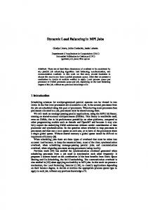
Fig. 5.
TABLE VI S TATISTICAL M EASURES [ SEC ] OF M AXIMUM T IME VARIATION OF W ORKLOAD M EASURE IN E NGINE S IMULATIONS
An Example of Grid Dynamic Partitioning Dynamic Distribution of Grid Cells small grid
1080
Proc 4 Proc 3 Proc 2 Proc 1
945
grid dynamic partitioning
E d r
Case 1 0.37 20.29 319.64
Statistical Measures small grid Case 2 Case 3 0.17 0.35 69.83 7.98 1232.52 69.0
of {v(s)}s=1,...,S large grid Case 1 Case 2 Case 3 0.47 0.55 0.261 40.05 14.26 806.66 221.19 136.08 10485.25
Summarizing the results we think that our dynamic load balancing algorithm works good especially on the following couples “(size grid,test case)”: (small grid,Case 3) and (large grid,Case 2). For the other simulations, especially for (small grid,Case 2) we point out that we defined (5), assuming {T s (i)}i=1,...,N as a good estimate of the computational workload unit for the next time-splitting interval s + 1. This hypothesis is not realistic in the case of very rapid reactions as these happen especially in the starting phase of the combustion process. In order to support this guess we measured the distribution values of {v(s)}s=1,...,S , i.e. the maximum time variation of the workload measure on two consecutive timesplitting interval for all the simulations in each test case and for both available grid sizes:
0 crank
imbalancing reduction with respect to pure block distribution on 64 processors for Case 1 from 36% to 18% and for Case 2 from 40% to 11%. On the other hand, Case 2 does not take benefits by introduction of the dynamic strategy in data partitioning. It shows comparable performances as pure block distribution, but an increasing of workload imbalancing for all the numbers of processors except for p = 64. Furthermore, on this simulation we note that, while µ indicates a reduction of global imbalancing, RG measures an increasing of imbalancing on the global simulation, when the dynamic strategy is employed. We can make similar analysis for large grid, indeed we can see in Table II for all the three test cases a reduction of the execution times for each number of processors. In this case the introduction of dynamic load balancing leads to an improvement of performances of the combustion solver for all the three test cases, as it is inferred by Fig. 3 and Fig. 4, where we show speed-up and efficiency of dynamic distribution (vs pure block distribution) on large grid. We see a speed-up of about 56 for Case 1 and of about 51 for Case 2 on 64 processors, which correspond to a parallel efficiency of about 88%and 79%, respectively. In these test cases, as shown on the bottom part of Table V, we obtained a reduction of imbalancing from 44% to 30% for Case 1 and from 31% to 15% Case 2. For Case 3 we obtained a slight improvement of performance corresponding to a considerable reduction of imbalancing workload except for p = 32 and p = 64. In all the test cases we observed that for all the numbers of processors, the number of time-splitting intervals where the definition of (4) does not complete the indeces set I is very small. On small grid it is about 3% for all the test cases, while on large grid it is about 4%, 1% and 2% for Case 1, Case 2 and Case 3, respectively. So the assignment of extra grid cells to the last processor produces a load imbalancing in a very few splitting intervals and it can not to be the reason of significative performance degradation during the simulations. A snapshot of grid distribution, when the dynamic algorithm is used for small grid and P = 4, is shown in Fig. 5.
v(s) := max
i=1,...,N
" s+1 # |T (i) − T s (i)|
s = 1, . . . , S
(8)
Statistical properties of these distributions are shown in Table VI, where E is the mean value, d is the standard deviation and r is the range of data distribution. Measures of Table VI, on one side, validates the good results of the dynamic load balancing algorithm especially for (small grid,Case 3) and (large grid,Case 2), on the other side, confirms that the time variation in workload distribution between two consecutive time-splitting intervals cannot be negligible, especially for (small grid,Case 2) and (large grid,Case 3), where the range of {v(s)}s=1,...,S points out a great difference between T s (i) and T s+1 (i) for a large number of intervals. In conclusion, starting from the above preliminary results, we believe that our dynamic approach gives interesting improvement in the parallel efficiency and scalability of our parallel software. However, since (5) can be an unreliable measure of grid cell workload when combustion phenomena are very quick, we are going to introduce in (5) a measure of the time variation of the workload in two consecutive time-splitting intervals. VII. C ONCLUSIONS In this work we have shown first results about the introduction of a dynamic load balancing algorithm in a parallel combustion solver, using a strategy which preserves contiguousness of the computational grid cells. The contiguousness is necessary when the combustion task is part of a multicomponent code for engine simulations, in which solvers for the Partial Differential Equations (PDEs) driving the fluid flow require frequent interactions among contiguous grid cells. 139
Numerical experiments have been carried out on three different operative conditions of an engine and on two different size of a discretization grid representing engine geometry. In general, numerical results have shown considerable improvement in efficiency with respect to pure block distribution. However, in few cases the algorithm does not produce an improvement, this is due to definition of the workload measure. Indeed, the employed measure of the computational workload unit does not consider the time variation in two consecutive timesplitting intervals, and this is an important aspect in the case of very rapid reactions. Therefore, we are investigating for a modified definition of the workload measure also taking into account time variation. R EFERENCES [1] A. Ali, G. Cazzoli, S. Kong, R. Reitz, C.J. Montgomery, Improvement in Computational Efficiency for HCCI Engine Modeling by Using Reduced Mechanism and Parallel Computing, 13th International Multidimensional Engine Modeling User’s Group Meeting, 2003. [2] A.A. Amsden, KIVA-3V: A Block-Structured KIVA Program for Engines with Vertical or Canted Valves, Los Alamos National Laboratory Report No. LA-13313-MS, 1997. [3] L. Antonelli, P. Belardini, P. D’Ambra, F. Gregoretti, G. Oliva, A Distributed Combustion Solver for Engine Simulations on Grids, Journal of Computational and Applied Mathematics, Elsevier, 2008. [4] P. Belardini, C. Bertoli, S. Corsaro, P. D’Ambra, Parallel Simulation of Combustion in Common Rail Diesel Engines by Advanced Numerical Solution of Detailed Chemistry, in: Applied and Industrial Mathematics in Italy, Proc. of the 7th Conference of SIMAI, M. Primicerio, R. Spigler, V. Valente eds., World Scientific Pub., 2005. [5] P. Belardini, C. Bertoli, S. Corsaro, P. D’Ambra, Multidimensional Modeling of Advanced Diesel Combustion System by Parallel Chemistry, Society for Automotive Engineers (SAE) Paper No. 2005-01-0201, 2005. [6] P.N. Brown, G.D. Byrne, A.C. Hindmarsh, VODE: A Variable Coefficient ODE Solver, SIAM Journal on Scientific and Statistical Computing, 10, 1989. [7] K.D. Devine, E.G. Boman, R.T. Heaphy, B.A. Hendrickson, New Challenges in Dynamic Load Balancing, Applied Numerical Mathematics, Elsevier, 2004. [8] I. Foster, Designing and Building Parallel Programs, Addison-Wesley, 1995. [9] G.W. Gear, Numerical Initial Value Problems in Ordinary Differential Equations, Prentice-Hall Englewood Cliffs NY, 1973. [10] J. Gustavsson, V.I. Golovitchev, Spray Combustion Simulation Based on Detailed Chemistry Aprroach for Diesel Fuel Surrogate Model, Society for Automotive Engineers (SAE), Paper No. 2003-0137, 2003. [11] E. Hairer, G. Wanner, Solving Ordinary Differential Equations II. Stiff and Differential-Algebraic Problems, Second Edition, 14, SpringerVerlag, 1996. [12] R.J. Kee, F.M. Rupley, J.A. Miller, CHEMKIN-II: A Fortran Chemical Kinetics Package for the Analysis of Gas-phase Chemical Kinetics, SAND89-8009 Sandia National Laboratories, 1989. [13] P. K. Senecal, E. Pomraning, K. J. Richards, T. E. Briggs, C. Y. Choi, R. M. McDavid, M. A. Patterson, Multi-dimensional Modeling of Direct-Injection Diesel Spray Liquid Lenght and Flame Lift-off Lenght using CFD and Parallel Detailed Chemistry, Society for Automotive Engineers (SAE), Paper No. 2003-01-1043, 2003. [14] M. Snir, S. Otto, S. Huss-Lederman, D. Walker, J. Dongarra J.: MPI: The Complete Reference, available in http://www.netlib.org./utk/papers/mpibook/mpi-book.html, 1993. [15] C.Z. Xu, F.C.M. Lau: Load Balancing in Parallel Computers: Theory and Practice, Academic, 1997.
140