an example of its usefulness, the new fuzzy border distance ... The distance between a pixel in the ... to-right and top-to-bottom, the other from right-to-left and.
Fuzzy border distance transforms and their use in 2D skeletonization Gunilla Borgefors Stina Svensson Centre for Image Analysis Swedish University of Agricultural Sciences L¨agerhyddsv¨agen 17, 75237 Uppsala, SWEDEN gunilla,stina @cb.uu.se �
Abstract Segmentation is always a difficult task in image analysis. In this paper, we propose a solution to computing distance transforms in images with fuzzy object borders. The difference from a standard distance transform is in the initialisation, which takes the fuzziness of the border into account. As an example of its usefulness, the new fuzzy border distance transform is used in skeletonization.
1. Introduction Distance transforms (DT) are useful tools for many types of shape representation, manipulation, and analysis. The earliest presentation of DTs, the city block and chessboard DTs, are found in [7]. The distance between a pixel in the object (background) to the background (object) is there defined as the number of steps in the shortest path between the pixel and any pixel in the background, where permissible steps are those between neighbouring (4-neighbour or 8-neighbour) pixels. The concept has then been extended to weighted DTs (WDT), using different weights for different steps, [2]. Another development is using larger neighbourhoods, [2, 10]. WDTs have also been investigated for three-dimensional images, [4]. However, all DTs assume that the object/background segmentation is perfect and that the input is a binary image. (The only example we found where the grey-level value is taken into account is [8]. There the DT labels in the background depend on both the distance from an edge and the strength of that edge.) Often, segmentation is a difficult problem, perhaps the most difficult problem in shape based image analysis. It would be preferable to compute the DT on the unsegmented image. We consider grey-level images where the separation into object and background is simple except for a number of voxels placed in the regions
of the border of the object. Any threshold (not necessarily on grey-level, but on any classification measure) would give a “noisy border”, that will make subsequent analysis, e.g., skeletonization, difficult. This is a very common situation in many medical and industrial applications. The idea behind the new WDT, called fuzzy border WDT (fbWDT), is that the initialisation of the distance transformation will be altered compared to the standard case. In the standard case, object pixels are set to infinity and background pixels to zero. In the fbWDT, the initialisation will reflect the uncertainty of the border pixels. Then the standard chamfering technique is used to compute the fbWDT in two raster scans of the image, the first from leftto-right and top-to-bottom, the other from right-to-left and from bottom-to-top, see, e.g., [2]. The fbWDT is easily ex, tendible to WDTs using larger neighbourhoods than and to three dimensions. The fbWDT can be used in any application utilising DTs, in (almost) the same way as a standard DT. In principle, it could also be used for the Euclidean DT, [6], but it is less straightforward to determine a reasonable initialization. To illustrate the usefulness of the fbWDT, we will present a skeletonization algorithm. We will both show that it improves the result compared to using a single threshold and how the skeletonization algorithm must be modified to work on the fbWDT. �
�
�
2. Fuzzy border distance transforms , have a black object Assume that we, in the real plane on a white background. Assume that this object is digitised into . If we directly create a binary image, we can either adopt the principle that any pixel whose centre is black will be black or the principle that any pixel whose area is more than half black is black. In any case, the object border will become jagged. In Figure 1(a), the situation is shown for a very simple geometry: the vertical border between object �
�
1051-4651/02 $17.00 (c) 2002 IEEE
�
background
are distributed linearly nitely object. The integer labels for pixels with values between the thresholds. The threshand should be set “symmetrically”, so that the olds best possible threshold corresponds to the middle of their range, i.e., to position in Figure 1(b). Therefore, we can are (and will) assume that pixels with initial labels most plausibly background and those with labels are most plausibly object. In Figure 2, left, a part of a grey-level image is shown and in the middle the initialisation we get if and . Once the image is inifor tialised in this new way, the DT is computed in the standard way. In Figure 2, right, the fbWDT is shown. As mentioned in the Introduction, the fbWDT is easily extendible to larger neighbourhoods and to higher dimensions. For all fbWDTs, the weight for steps between edge-neighbours (face-neighbours in 3D) should not be too low, as then we have too few labels free to distribute on the border. This is not the situation for WDTs, where we want a low . Therefore, suitable weights for fbWDTs can not readily be found in the literature. In Table 2, and neighgood choices of WDTs for the neighbourhood in 3D are bourhoods in 2D and summarized. In , denotes the knight-neighbour and in , , , and denote the face-, edge-, and vertex-neighbours, respectively. The maximal difference from the Euclidean distance, maxdiff, in an image of size is listed. The fbWDT is very similar to a standard WDT, except on the border of the object. There it is not ordered in any way. Due to noise, a more internal pixel can have a lower value than a more external one. In this case, the fbWDT label of the more internal pixel will be lower than that of the situathe more external one. For fbWDT labels tion is well-behaved, as in a standard WDT. The fact that ) can be disordered means that some the border pixels ( adjustments may become necessary in algorithms where the DT is utilised. %
object
!
�
�
�
�
�
�
�
�
�
�
�
�
�
�
�
�
�
�
�
�
�
�
�
�
�
�
�
�
�
�
�
�
�
�
�
�
�
�
�
�
�
�
�
�
�
�
�
�
�
!
"
�
#
�
%
�
*
�
�
�
�
�
�
�
vwx y z
!
I
(a)
(b)
�
�
,
.
!
#
�
(
�
,
�
�
Figure 1. Principle for initialisation. See text.
"
�
(
�
�
�
�
�
Table 1. Initialisation. See text and Figure 1. value initialisation binary grey binary grey left right left right left right left right 0 1 0.4 1 0 2 0 1 0.2 1 0 1 0 1 0 1 0 0 0 1 0 0.8 0 0 4 0 1 0 0.6 0 0 3
�
�
�
�
�
�
�
�
�
�
�
�
�
�
7
7
�
and background is straight and falls somewhere between two pixel centres. The border can be placed in a rather large interval, , giving the same digitisation — a background pixel to the left and an object pixel to the right. neighbourhood WDT, denoted , In a is the weight for steps between edge-neighbours and the weight for steps between point-neighbours. We will here use . The smallest distance label we can have is 5. never occur. They are thus free to be The labels used to initialise the fuzzy border, so that the position of the border in the interval , Figure 1(a), does make a difference. In Figure 1(b), the border is placed in five different . The “ideal” one, where the digitipositions, sation is “perfect” is position in this case. The left pixel should be initialised to zero and the right to . For the other positions, see Table 1. There, for each border position, the binarisation of the left and right pixels in Figure 1, the relative area of the pixel that is covered by the object, the initialisation for the binary case and the suggested iniare listed. The position of the tialisation for the border does now influence the DT labels. In practise, we do not know where the real border actually is, but can use the grey-level (or some other classification measure) as an indication. The general initialisation is done as follows. Two thresholds are used: values below are definitely background and values above are defi
�
�
�
�
�
�
�
�
�
�
�
�
�
�
�
�
�
�
�
3
�
5
�
3
�
�
�
�
�
�
�
�
�
�
3
�
�
3
�
�
�
�
�
�
�
�
8
7
9
�
;
%
�
�
�
�
�
�
�
�
�
�
�
�
!
"
3. 2D Skeletonization
�
�
!
#
The fbWDT can be used in all cases where WDTs are used. As an illustration, we use 2D skeletonization. In [9], a skeletonization algorithm for 2D binary images is introduced. It is based on iterative thinning guided by a DT. This skeleton can be computed using any DT and fulfils the skeletal properties, i.e., the skeleton is a thin subset of the object, is topologically equivalent to the object, is centred within the object (with respect to the distance represented by the DT), and is reversible (i.e., allows complete reconstruction of the object). Each pixel in the DT can be interpreted as the centre of a disc, fully enclosed in the object, with radius equal to the label of the pixel. A pixel whose corresponding disc is not
1051-4651/02 $17.00 (c) 2002 IEEE
49 50 44 53 44 56 58 57 50 49 63 56 51 54 49 50 48 51 51 51 66 66 77 61 59 67 60 52 52 56 74 74 81 79 74 74 67 61 53 57 76 79 67 79 68 83 76 77 61 58 73 73 76 80 81 77 77 78 76 76 78 76 73 76 67 71 78 66 73 72 81 62 55 59 53 69 65 70 69 76 68 72 57 60 49 49 42 63 68 67 76 77 63 59 53 48 52 48 50 55
. . . 1 . . 2 2
. . .
3
. . .
. . . . 3 . 3
. . . .
. . . . .
3
1 . . 3 . . 1 .
3 . . .
. . . . .
. . 1 . 2 2 7 7 12 8 13 10 8 6 6 1 3 5 8 6
4 2 3 2 4 3 . . 1 3 3 . . . . .
. . 5 7 3 8 5 . . 1
. . . 5 8 10 5 . . .
. . . 5 3 8 3 . . .
. . 3 7 8 9 4 3 . .
. . . 3 7 9 7 2 . .
. . . . 5 7 2 4 1 .
. . . . . 5 7 3 3 .
. . . . . 5 7 8 3 .
Figure 2. Grey-levels; initialisation of the fbWDT; the resulting fbWDT. ponents in the neighbourhood of , except when all four edge-neighbours of are object pixels. If , the removal of does not break the 8-connectedness of the object. A simple skeletonization algorithm similar to the one described in [9] can be summarised as follows. Start by computing the DT. On the DT, the CMDs are detected. After that the DT is repeatedly investigated. Each iteration consists of two subiterations. During the first, all pixels with label that has an edge-neighbour in the back, and is not a CMD are marked simultaground, neously. During the second, marked pixels with are removed sequentially. The two subiterations have to be repeated once, except for city block DT. To extend the algorithm to fbWDT, we first need to identify the CMDs. This is done analogously to the detection of CMDs for the WDT, i.e., values are replaced in the same way as for the WDT and then (1) is used. The only differ, as they are most likely ence is that pixels labelled to belong to the background, are never regarded as CMDs. labels 1 or 2 will not be considered CMDs.) (For As already pointed out, there is no ordering among the labels for pixels placed in the border area of the object, . This means that special rules have to i.e., for labels be used when the marking and removal is iterated. The genas background eral idea is to treat pixels with label (and those as object). However, when these pixels are placed inside the object, i.e., are surrounded by pixels with higher labels, they are kept (at least temporarily) to avoid creating spurious holes. are directly removed, label afPixels with label ter label, if they have an edge-neighbour in the background, , the same i.e., with label zero. For pixels with label marking and removal is used as for the DT, with the only , pixels with label difference that in the computation of are considered as object only if they have no edgeneighbour in the background. After each iteration , i.e., after pixels with label have been examined, we again process the pixels with label . This will allow removal of pixels that were kept in previous iterations as they were then surrounded by pixels with higher labels. For a quick �
Table 2. Good choices of weights for fbWDTs.
'
(
,
�
�
�
maxdiff
2D DT
3D DT
maxdiff
. �
�
�
� �
�
� �
�
�
�
�
�
5
�
�
�
�
�
�
�
�
�
�
�
�
�
�
� �
�
�
�
�
�
�
�
5 �
�
�
�
�
�
�
�
�
�
�
�
�
�
5
�
�
�
� �
�
�
�
�
�
�
�
.
�
�
�
�
<
�
�
�
�
�
�
�
�
�
�
�
5 �
�
�
�
�
�
�
<
�
�
�
� �
�
�
�
�
�
'
�
�
�
�
�
�
�
�
,
(
�
�
� �
'
�
�
�
�
�
�
�
�
(
,
�
�
�
�
�
�
�
� �
�
�
�
�
�
�
completely covered by the disc of any other pixel in the object is called a centre of a maximal disc (CMD). The union of the discs corresponding to the CMDs coincides with the original object. The CMDs can be identified by inspecting the DT, [1, 3]. A pixel is a CMD if all its neighbours have lower or equal label, taking into account the weight for the step to the corresponding neighbour. The numbering , is counter-clockwise, of the neighbours , starting from the edge-neighbour to the right of . A pixel is a CMD in if for all , with proper weights �
,
�
�
�
�
�
�
�
�
�
�
,
�
�
�
�
�
� �
�
�
� �
�
�
(1) �
�
�
% �
�
� �
%
�
�
,
�
�
�
�
#
�
�
8
9
�
�
�
�
�
�
�
�
�
�
�
�
�
�
3
�
5
�
�
�
�
3
�
�
�
2
,
�
�
3
�
5
/
4
,
'
(
8
9
,
*
�
�
�
-
�
�
,
�
,
+
�
�
�
�
�
�
8
/
�
/
�
�
'
(
8
�
9
is equal to the number of 8-connected object com-
(
�
�
�
�
%
�
%
;
Unfortunately, (1) is not valid for small labels. The largest label not occurring in is , [3]. have to be replaced by the smallest label Values below it that does not occur, [1]. For , e.g., pixels with label 5 are replaced by 1 and pixels with label 7 by 6 in , while the situation (1). The same rules apply for is more complex for , see [3]. Topology preservation, with respect to 8-connectedness of the object, can be checked using the Hilditch crossing number, [5], if and ( or ) otherwise
�
�
(
�
(
�
�
%
�
(
�
;
%
'
�
(
�
(
�
(
�
1051-4651/02 $17.00 (c) 2002 IEEE