Fuzzy Constraints, Choice, and Utility Philippe De Wilde Intelligent and Interactive Systems Group Department of Electrical Engineering Imperial College of Science Technology, and Medicine London SW7 2BT, United Kingdom
[email protected] Abstract— We revisit the notion of fuzzy revealed preference, with the intention of using it in decision making. A decision making agent manages resources that are priced, and it has a certain wealth. We review proposed fuzzifications of preference relations. Although they are well founded, they cannot deal well with decision making under fuzzy constraints. We introduce the fuzzy budget set as a general model of fuzzy constraints on resources. We then show that a general condition for rationality, the fuzzy axiom of revealed preference should not be an axiom anymore, but just a statement that is true to a certain degree. We show how to calculate this degree of truth. We define a fuzzy utility function, and show how it can be maximised, subject to fuzzy budget constraints. Keywords— fuzzy choice, fuzzy utility, fuzzy budget, qualitative reasoning
I. Fuzzy choice and intelligent agents
E
LECTRONIC commerce allows buyers and sellers to use increasingly complicated decision procedures. Large amounts of information are available, and computers can process this to advise the economic agent in the choice of an alternative. The information gathered, over the web for example, is often inconsistent. If it is to be used in decision making, the decision making process will have to be able to deal with uncertainty. Humans deal with uncertainty in a natural way, via generalization. Automatic procedures use either probability theory or fuzzy logic. We prefer fuzzy logic because it deals with linguistic variables in a more intuitive way that probability theory. The linguistic variables are classes that have evolved over time, in a certain application domain, to be effective in generalization. Linguistic variables are the method adopted by humans to indicate choice and preference. Many intelligent agents aim to capture the preferences of their human owner. If decisions are to be made by a computer agent in e-commerce, it is essential that the computer agent agrees with the human owner. Should we study psychology before implementing a shop-bot? This would create problems, as a psychological analysis of economical behaviour returns results that are difficult to implement in a computer algorithm. Most economists hold that their theory, micro-economics based on game theory, gives an accurate description of human economical behaviour. They even have applied the microeconomic paradigm to areas such as social interactions, and irrational behaviour in households and firms [1]. For
the management of resources, a core economic activity, the micro-economic approach is prevailing. This is what e-commerce is mostly about: buying and selling quantifiable resources. If we can allow the quantities to be fuzzy, e-commerce and e-management of resources will be even more widely applied than it is now.
E-commerce and e-management of resources can operate automatically using intelligent software agents. To achieve this, we need to re-formulate micro-economy so that it can deal with fuzzy choice and preferences. The Orlovsky choice function is often used as the basis for fuzzy choice [2], [3]. We will start from an entirely different starting point, immediately taking into account prices of resources that affect the choice among alternatives. Another approach, ranking based on pairwise comparisons is described in [4]. Choice among attributes that have multiple attributes is reviewed in [5]. The attributes of our alternatives will be the prices of goods in the consumption bundle. This will allow us to have more specific procedures for ranking than in [5], [4].
Once a basic concept, such as the Orlovsky choice function is proposed and adopted, scientists usually start refining and generalizing it. This happened to fuzzy choice functions, just as it happened to Nash equilibrium, expert systems, etc. Much of the current theory about fuzzy choice has become so abstract that it is impossible to implement in an e-commerce agent. The refined theory of choice can certainly be used to model particular user’s decisions very accurately, but this matching of theory and user requires extensive human intervention. If the e-commerce agent has to implement fuzzy choice automatically for a large class of users, we have to turn back, and use a more intuitive theory. Kulshreshtha and Shekar [6] have recently attempted to present an intuitive perspective on fuzzy preference. It becomes clear from this paper that there is an array of possible choice functions, with no clear criteria as to which ones to prefer. There are even some intuitive contradictions. The authors point out the need to conduct experiments to find the most appropriate fuzzy preference relations for real life situations. We will not conduct experiments, but consider the crisp theory of preference closer to the application (resource management), before fuzzifying it.
II. Two weak axioms of fuzzy revealed preference We now explain the theory of choice, based on [7], and its fuzzification, based on [8]. In the next section, we will propose a radically different fuzzification. The set of alternatives is called X. A preference relation º: X 2 → {0, 1} assigns the number 0 or 1 to two alternatives x and y, where x º y means that alternative x is at least as good as y, in other words, x weakly dominates y. The strict preference relation  is defined by x  y ⇔ x º y but not y º x. On the same set of alternatives X, the standard fuzzy preference relation R(x, y) : X 2 → [0, 1] indicates the degree to which x is at least as good as y, a number between 0 and 1. It is clear that the crisp preference relation º is the limit of the fuzzy preference relation R, where the degree can only take on values 0 or 1. Often, more than one alternative is acceptable. It is not possible to implement this via a function; hence the concept of choice structure was introduced. A choice structure is denoted by (B, C). Here B is a set of nonempty subsets of X. An element B ∈ B is called a budget set. It consists of a number of alternatives. C is a choice rule that assigns a non-empty set of chosen elements C(B) ⊂ B for every budget set B. It represents the choice made by the agent of one or more alternatives from the set B ⊂ X. These alternatives are acceptable alternatives to the agent. A fuzzy choice rule assigns a non-empty fuzzy set of chosen elements C(B) ⊂ ∼ B for every budget set B. A fuzzy subset is defined in the standard way as C(B) ⊂ ∼ B ⇔ µC(B) (x) ≤ µB (x), ∀x ∈ X,
(1)
where µB indicates the membership function of a set B. This reduces to the crisp notion of subset, when the membership functions can only take on the values 0 or 1. For this reason the fuzzy choice function is a simple extension of the crisp one, and we will denote both by (B, C). A choice structure induces a preference relation called the revealed preference relation º∗ defined as follows: x º∗ y ⇔ ∃B ∈ B|x, y ∈ B and x ∈ C(B),
(2)
where we read x º∗ y as “x is revealed as least as good as y”, meaning that both alternatives have to be in a budget set, with the preferred one also in the choice set. Remark that the other alternative can also be in the choice set. It is again possible to define the strict preference relation x Â∗ y ⇔ x º∗ y but not y º∗ x.
(3)
The revealed fuzzy preference relation is defined as follows (following [8], but with our notation) R∗ (x, y) =
max
{B|x,y∈B}
µC(B) (x).
(4)
This definition reduces to (2) for membership functions that can take on only the values 0 and 1, but it is only one amongst many possibilities. It is even possible to
use linguistic variables for the values of R∗ , as in [9]. The linguistic variables have to be defined by membership functions, that can be related to µC(B) . Differences in the literature, and counter-intuitive definitions start when one tries to define fuzzy strict preference relations, the fuzzy equivalent of x  y. A fuzzy strict preference relation can be defined as P ∗ (x, y) = max[R∗ (x, y) − R∗ (y, x), 0].
(5)
This makes the relation P ∗ (x, y) anti-symmetric, as is required for a strict order. In [8], the proposal for a fuzzy strict preference relation is P ∗ (x, y) =
max
[µC(B) (x) − µC(B) (y), 0].
{B|x,y∈B}
(6)
For this relation P ∗ , we have to find a definition based on fuzzy choice rules. Remark that in (4) and (6), the maximum is taken over all budget sets B containing x and y, but R∗ (x, y) is independent of the degree to which y is in the fuzzy choice set C(B). It is the function P ∗ that will be used in the formulation of one of the most fundamental axioms of in the theory of choice, the weak axiom of revealed preference [10]. The weak axiom of revealed crisp preference states that Axiom 1 (Crisp weak axiom) If for some B ∈ B with x, y ∈ B we have x ∈ C(B), then for any B 0 ∈ B with x, y, ∈ B 0 , we must also have x ∈ C(B 0 ). This means that, if there are two budget sets both containing two alternatives, and one alternative is chosen in the first set, and the second alternative is chosen in the second set, then the fist alternative must also be chosen in the second set. This is an intuitive way of requiring consistency. In terms of revealed preferences, this means that, within a given choice structure, if x is revealed at least as good as y, then y cannot be revealed to be strictly better than x. The weak axiom of revealed fuzzy preference exists in two forms ([8], our notation) Axiom 2 (Fuzzy weak axiom, version 1) For all alternatives x and y, P ∗ (x, y) > 0 implies R∗ (y, x) < 1. Axiom 3 (Fuzzy weak axiom, version 2) For all alternatives x and y, and for all 0 < k ≤ 1, P ∗ (x, y) > k implies R∗ (y, x) < 1 − k. These two fuzzy axioms are not intuitive, and are not generalizations of the crisp axiom. We try to remedy this in the next section. III. Weak property for revealed fuzzy preference for budget sets Assume an agent manages L resources, and has quantities x1 , . . . , xL of them. The resources have prices p1 , . . . , pL . These prices can also be virtual, for example when networked agents manage tasks, or when the resources are intangible. However abstract the resources may be, we feel that for agents in an e-commerce context, they can always be quantified and priced. As we study multi-agent systems with many agents, the price will be determined by the market, not by a single agent. The resource vector is denoted by x, and the price vector by p. The agent has a level of wealth w. This can
(w − px + d(w)), w ≤ px ≤ w + d(w), 0, w + d(w) ≤ px, d(w)
(7)
2
µ (4−3x −5x )
1 B
0.4 0.2 0 2 1
1.5 0.8
1
0.6 0.4
0.5 0
x2
0.2 0
x
1
Fig. 1. A piecewise linear fuzzy budget set for two goods in quantities x1 and x2 , and with prices 3 resp. 5. The wealth limit equals 4 and can be exceeded by 1.
1 0.8 2 1
0.6
B
0.4 0.2 0 2 1
1.5 0.8 0.6 0.4
x2
0
0.2 0
x1
Fig. 2. A smooth fuzzy budget set for two goods in quantities x1 and x2 , with prices 3 resp. 5. The wealth limit 4 can be exceeded to an arbitrary amount.
1 {tanh[δ(w)(w − px)] + 1}, 2 δ(w) > 0.
0.6
0.5
and µB (w, w − px) =
0.8
1
1, px ≤ w, 1 µB (w, w − px) =
1
µ (4−3x −5x )
again be virtual or real, and expresses the buying power or power to recruit other agents, that an agent has. The resources that an agent can afford are usually calculated from the Walrasian [7] budget set {x ∈ X : px ≤ w}. As the decision making by software agents in e-commerce is exclusively governed by such constraints, we feel that the Walrasian budget set is the right concept to fuzzify, not the choice function. We will denote by µB (x) the degree to which an alternative x ∈ X belongs to the budget set. The fuzziness arises because the inequality constraint px ≤ w may only hold to a certain degree. It is the leniency that your banker shows you, or the degree to which a company is willing to break its rules to satisfy customers. This flexibility is necessary to break deadlocks. Humans show it, and economic software agents have to have it as a feature. The function µB depends on the alternatives in a special way. The flexibility has to be a function of the difference w − px, because this is the budget surplus or budget deficit. This difference shows how much capability the agent still has (w > px), or whether it has exceeded its wealth. The degree µB will also depend directly on the wealth, for this allows us to take into account such facts as that a small deficit is irrelevant if the wealth is large, etc. On the other hand, µB should not depend directly on p or x. This is because µB is only concerned with wealth, not with prices per unit, or units of resources, the latter two being of a different dimension from w. Moreover, the prices are set by the market, but the tolerance for px to exceed w depends only on the individual decision maker. Two particularly useful functions for µB are
(8)
We will call such membership functions fuzzy budget constraints or resource constraints interchangeably in the sequel. Function (7), illustrated in figure 1 indicates that all alternatives x that are in the crisp Walrasian budget set, are in the fuzzy budget set to a degree one. This degree then decreases linearly to 0 until px exceeds w + d(w). The quantity d(w) indicates the flexibility of the wealth limit w. Function (8) illustrated in figure 2 decreases gradually from near 1 to near 0 as px increases, taking the value 1/2 when px = w. The slope δ(w) indicates how hard the budget constraint w is, with a hard constraint implemented via a large δ(w). Walras’ law, px = w for all x, can be exactly satisfied by (7), when µB = 1, but will never be exactly satisfied for (8), where µB can only approach 1 asymptotically. Any linear transformation of prices p or resource
amounts x will preserve the membership functions (7) and (8) in the same form. For the same reasons, any hyperplane in the L-dimensional x-space will cut the surfaces (7) and (8) according to a piecewise linear or a tanh function respectively. The Walrasian demand correspondence x(p, w) is the amount of goods x at prices p that can be consumed given wealth w. Normally this is a point within the budget set, or on the edge of the budget set if Walras’ law px = w is fulfilled. If the budget set is a fuzzy set µB , we define the demand correspondence as a fuzzy set with µ(x, p, w) = µB (w, w − px). (9) Many different amounts of good can be consumed, each to a different degree. If µB (w, w − px) = 0, then x(p, w) cannot be consumed. The Walrasian demand correspondence x(p, w) is homogeneous of degree zero if x(αp, αw) = x(p, w) for any p, w and α > 0. In the fuzzy version, homogeneity of
µW (x) = min{µB [w, w − px(p0 , w0 )], (10) 1 − µB 0 [w0 , w0 − p0 x(p, w)]}. An illustration is given in figure 3. It can be shown that if the budget sets are crisp, the fuzzy weak property always holds to a degree 1, hence is always true. So instead of a fuzzification of the crisp weak axiom, as axioms 2 and 3 at the end of section II, we have found not an axiom, but a property. This property holds to a certain degree. If the membership function of the budget set is ’flat’, then the ridge in figure 3 will not be very pronounced, indicating indifference in the choice of consumption bundle x(p, w). On the other hand, if µB drops sharply at px = w, the ridge will be clearly defined. The fuzzy budget set and the fuzzy weak property have given us an intuitive approach to fuzzy constraints, without the necessity to define fuzzy preference relations. In the next section we will show how the fuzzy budget set can be combined with utility maximization. IV. Fuzzy utility maximization under fuzzy resource constraints Once constraints on resources are laid down in a budget set, the next step is to maximize utility, given a budget set. Fuzzy constraints go together with fuzzy objectives. The latter can be modeled by a fuzzy utility function. Fuzzy utility functions have been introduced via fuzzy random variables [11], in a desire to find a
0.8 0.6 µW(x1,x2)
degree zero becomes a property of the membership function µB of the fuzzy budget set. It can easily be seen that (7) and (8) will be homogeneous of degree zero if d(w) respectively δ(w) are constants, this means that the flexibility on the budget constraint is independent of the wealth. The Walrasian demand correspondence is different from a price-wealth situation x(p, w). The price-wealth situation is simply the actual consumption of goods x at prices p and wealth w, all crisp numbers. There is nothing fuzzy about a price-wealth situation. The demand correspondence however is fuzzy, because of the fuzzy budget set. It is the originality of our approach that we only introduce fuzziness via fuzzy budget constraints, and not via fuzzy choice relations. Now that the resource constraints are formulated as a fuzzy budget set µB , we are able to formulate a much more intuitive fuzzy weak axiom. The crisp weak axiom of revealed preference for a Walrasian demand function x(p, w) is Axiom 4 (Crisp weak axiom) For any (p, w) and (p0 , w0 ), if px(p0 , w0 ) ≤ w and x(p0 , w0 ) 6= x(p, w), then p0 x(p, w) > w0 . It can be shown [7] that this is equivalent to axiom 1. The fuzzy version can now be obtained in an intuitive way, if the membership function µB is introduced. Property 1 (Fuzzy weak property) For any two fuzzy budget sets µB (w, w − px(p, w)) and µB 0 (w0 , w0 − p0 x(p0 , w0 )), and any two price-wealth situations x(p, w) 6= x(p0 , w0 ), the fuzzy weak property holds to a degree
0.4 0.2 −1 0
0 4
1
2
0 x
−2 2
x2
1
Fig. 3. Two resources, and two budget sets defined by x1 + x2 = 1 and x1 /2 + 2x2 = 1 (the two obliquely intersecting straight lines in the graph). Expression (8) with δ(w) = 1 is chosen for the membership functions µB of the two fuzzy budget sets. The degree to which the fuzzy weak property holds, µW (x1 , x2 ), is plotted, together with a projection of the contour lines. The ridge in µW coincides with the bisector of x1 + x2 = 1 and x1 /2 + 2x2 = 1.
treatment compatible with Bayesian statistics. Another approach is to use fuzzy numbers in an ordinary utility function [12]. Fuzzy graphs [13] are one of the most intuitive ways to quantify linguistic uncertainty, if the membership functions of the variables that are being related in the graph, are well known. Let the universe of discourse be quantities of the L resources. Instead of the numerical values x1 , . . . , xL , of the previous section, the decision maker uses linguistic variables with membership functions µli , i = 1, . . . , m, l = 1, . . . , L. For example, µ21 could be the membership function of a “small” quantity of resource 2, and µ22 the membership function for a “large” quantity of resource 2. The membership functions are functions of real numbers which we will denote by x1 , . . . , xL . The membership functions of the utility (“small utility”, “large utility” etc.) are denoted by µL+1 (xL+1 ), i i = 1, . . . , m. A fuzzy utility can now be defined as a fuzzy graph µU (x1 , . . . , xL , xL+1 ) = max min(µli (xi )). i
l
(11)
An example is given in figure 4. As the resource vector is also denoted x (and the price vector p), note that µU depends on x and xL+1 , the latter variable indicating the utility. If the utility is subject to budget constraints, the membership function will be the minimum of the utility and budget membership functions, min(µU , µB ). The
1
1
µU 2
µ2
0.8
0.8 µ21
0.6
µ11
0.6
µ12
0.4
0.4
0.2
0.2
0 3
0 3 3
2
3
2
2 1
2 1
1 0
x2
0
x2
x
1
Fig. 4. The fuzzy utility of a single resource (L = 1). A small amount of resource 1 has membership function µ11 , a large amount µ12 , low utility µ21 , high utility µ22 . The x1 variable is the amount of resource, the x2 variable quantifies the utility. In most practical applications there will be multiple resources.
utility maximization problem consists in choosing the resource allocation or consumption bundle x† that maximizes this minimum. x†
=
argmax min(µU , µB )
=
argmax min[µU (x, xL+1 ), µB (w, w − px)]
=
argmax min[max i
min
(12)
min[X, max(min(Y, Z), min(T, U ))] = (13)
The easiest way to prove this is by investigating the 32 different possibilities for ranking the variables X, Y, Z, T, U . It is possible to generalize (13) to i
We have now obtained an important, intuitive fuzzification of the crisp weak axiom for budget constraints on resources. In the crisp case, if an agent chooses the resource allocation x(p, w) over x(p0 , w0 ) whenever they are both available, x(p, w) must not be affordable at the price-wealth combination (p0 , w0 ) at which the agent chooses resource allocation x(p0 , w0 ). In the fuzzy case however, x(p, w) may be affordable. The fuzzy weak property (10) allows us to deal with agents that have relaxed budget constraints. In our view, this forms the basis of resource management with fuzzy restrictions. We have also show how utility can be maximized when the utility is fuzzy, and when there are fuzzy budget constraints. In the future, we plan to analyze fuzzy utility maximization as part of group decision making, along the lines of [14]. References [1]
Property (14) is important for fuzzy graphs with constraints. In words, it says that when a fuzzy graph is constrained (the minimum with X in (14)), this is equivalent to constraining the fuzzy relations (“rectangles”) that make up the fuzzy graph. We can now use (14) to simplify (12): x†
=
argmax max min(µli (xi ), µB (w, w − px)),
=
argmax min(µli (xi ), µB (w, w − px)),
i
i
l
1
where the last minimum is taken over L + 2 memberL+1 for ship functions: µ1i , . . . , µL i for the resources, µi the utility, and µB for the budget constraint. This is illustrated for L = 1 in figure 5.
min[X, max(min(Yi , Zi ))] = max(min(X, Yi , Zi )). (14) i
x
V. Conclusion
This fuzzy resource-constrained utility maximization problem is computationally intensive as formulated in (12), because of the succession of maximizations and minimizations. Fortunately it is possible to significantly simplify (12). This hinges on the observation that, for arbitrary numbers X, Y, Z, T, U ,
max(min(X, Y, Z), min(X, T, U )).
0
Fig. 5. The fuzzy utility of a single resource (L = 1), constrained by the fuzzy budget set of figure 2 and equation (7). The resource vector x† , here a single variable x†1 is that value of x1 where the fuzzy constrained utility is maximal. Compare this with figure 4: because of the minimization procedure, the second peak has disappeared, the remaining peak is lower and has a different slope.
(µli (xi ),
l∈{1,...,L+1}
µB (w, w − px))].
1 0
l
(15)
[2] [3] [4] [5]
Gary S. Becker, The Economic Approach to Human Behavior, University of Chicago Press, Chicago, 1976. Kunal Sengupta, “Fuzzy preference and Orlovsky choice procedure,” Fuzzy Sets and Systems, vol. 93, pp. 231– 234, 1998. Denis Bouyssou, “Acyclic fuzzy preferences and the Orlovsky choice function: a note,” Fuzzy Sets and Systems, vol. 89, pp. 107–111, 1997. Marc Roubens, “Choice procedures in fuzzy multicriteria decision analysis based on pairwise comparisons,” Fuzzy Sets and Systems, vol. 84, pp. 135–142, 1996. Rita Almeida Ribeiro, “Fuzzy multiple attribute decision making: a review and new preference elicitation
[6]
[7] [8] [9]
[10] [11]
[12]
[13] [14]
techniques,” Fuzzy Sets and Systems, vol. 78, pp. 155– 181, 1996. Pankaj Kulshreshtha and B. Shekar, “Interrelationships among fuzzy preference-based choice functions and significance of rationality conditions: a taxonomic and intuitive perspective,” Fuzzy Sets and Systems, vol. 109, pp. 429–445, 2000. Andreu Mas-Colell, Michael D. Whinston, and Jerry R. Green, Microeconomic Theory, Oxford University Press, Oxford, 1995. Asis Banerjee, “Fuzzy choice functions, revealed preference and rationality,” Fuzzy Sets and Systems, vol. 70, pp. 31–43, 1995. Marimin, Motohide Umano, Itsuo Hatono, and Hiroyuki Tamura, “Linguistic labels for expressing fuzzy preference relations in fuzzy group decision making,” IEEE Transactions on Systems, Man, and Cybernetics - Part B: Cybernetics, vol. 28, pp. 205–218, 1998. Amartya K. Sen, “Choice functions and revealed preference,” Review of Economic Studies, vol. 38, pp. 307– 317, 1971. Maria Angeles Gil and Pramod Jain, “Comparison of experiments in statistical decision problems with fuzzy utilities,” IEEE Transactions on Systems, Man, and Cybernetics, vol. 22, pp. 662–670, 1992. Chie-Bein Chen and Cerry M. Klein, “A simple approach to ranking a group of aggregated fuzzy utilities,” IEEE Transactions on Systems, Man, and Cybernetics - Part B: Cybernetics, vol. 27, pp. 26–35, 1997. Lotfi A. Zadeh, “Fuzzy logic, neural networks, and soft computing,” Communications of the ACM, vol. 37, pp. 77–83, 1994. Ronald R. Yager, “Penalizing strategic preference manipulation in multi-agent decision making,” IEEE Transactions on Fuzy Systems, vol. 9, pp. 393–403, 2001.