Progress In Electromagnetics Research, Vol. 118, 1–15, 2011
FUZZY-CONTROL-BASED PARTICLE FILTER FOR MANEUVERING TARGET TRACKING X. F. Wang, J. F. Chen, Z. G. Shi * , and K. S. Chen Department of Information and Electronic Engineering, Zhejiang University, Hangzhou 310027, China Abstract—In this paper, we propose a novel fuzzy-control-based particle filter (FCPF) for maneuvering target tracking, which combines the advantages of standard particle filter (SPF) and multiple model particle filter (MMPF). That is, the SPF is adopted during non-maneuvering movement while the MMPF is adopted during maneuvering movement. The key point of the FCPF is to use a fuzzy controller, which could imitate the thoughts of human beings in some degree, to detect the target’s maneuver and use a backward correction sub-algorithm to alleviate the performance degradation of MMPF caused by detection delay. Simulation results indicate that the proposed algorithm has a much better tracking accuracy than the SPF while keeps approximately equal computational complexity. Compared with MMPF, both algorithms have no tracking lost, but the tracking accuracy of the proposed FCPF is a little better than the MMPF, and the FCPF consumes about 66% computation time of the MMPF. Thus, the proposed algorithm offers a more effective way for maneuvering target tracking.
1. INTRODUCTION The problem of target tracking has been a hot topic for many years in the field of signal processing [1–4]. For linear Gaussian problems, the Kalman Filter (KF) can be applied to obtain optimal solutions; for nonlinear problems, Extended Kalman Filter (EKF) is usually implemented to provide an approximate solution [5]. In recent years, particle filter (PF) has been studied by many researchers since it was proposed in 1990s. The main idea of particle filter is to represent Received 19 May 2011, Accepted 14 June 2011, Scheduled 20 June 2011 * Corresponding author: Zhi-Guo Shi (
[email protected]).
2
Wang et al.
the probability density of system state by a set of particles with associated weights. It was shown in literatures [6–10] that particle filter is particularly suitable for estimating the state of nonlinear, nonGaussian dynamic system. All the target tracking methods mentioned above are model-based. Generally, it is difficult to use a single model to represent the motion of a maneuvering target, for the target is often abruptly deviated from the preceding motion. Hence, multiple model (MM) based approaches are often used for maneuvering target tracking to cover the true dynamics of the target. In all the MM based approaches, multiple model particle filter (MMPF) [11–13] is considered as an effective method for maneuvering target tracking at the present time for it combines the advantages of both multiple model and particle filter. The main idea of MMPF is to use multiple models to approach the true dynamics of maneuvering target. The MMPFs perform well when the models represent the true dynamic accurately, and are relatively robust when there are small modeling errors. However, these algorithms need as many predetermined sub-models as necessary to handle the varying target acceleration characteristics. This will not only incur extra computational complexity, but also lead to tracking accuracy degradation because of model competition [14], and therefor some of the models do not exactly match the target motion. In this paper, we propose an algorithm which combines the advantages of standard particle filter (SPF) and MMPF, that is, the SPF is adopted during non-maneuvering while the MMPF is adopted during maneuvering. In the proposed algorithm, the key point is maneuver detection which has been studied by many scholars [13, 14]. Many methods have been researched in [15]. Among these methods, the methods based on residual information are popular due to their high effectiveness and easy implementation [16]. This paper is also based on residual information. The main contribution of this paper is twofold. First, we use a fuzzy controller to imitate the thoughts of human beings to calculate the probability of maneuver starting according to the information contained in the so-called “sliding residual”. Second, a backward correction sub-algorithm is adopted to alleviate the performance degradation of MMPF caused by detection delay. The rest of this paper is organized as follows. Section 2 gives the mathematic model of a maneuvering target and a typical target trajectory. Section 3 describes the proposed FCPF algorithm, emphasizing on the maneuver detection process with fuzzy controller and backward correction sub-algorithm. Simulation results and discussions are presented in Section 4. Section 5 concludes this paper.
Progress In Electromagnetics Research, Vol. 118, 2011
3
2. MATHEMATIC MODEL OF TARGET Almost all maneuvering target tracking methods are model based. They assume that the target dynamics and its observation are represented by some known mathematic models. In the proposed FCPF algorithm, the state equation of the maneuvering target within the x-y plane is described as xk = A(T )xk−1 + Bu (T )uk + B(T )wk (1) y 0 x where xk = [xk , vk , yk , vk ] is the target state vector which contains the position and velocity of x and y directions; and for MMPF, the state equation becomes xkm = [xk , mk ]0 , where mk is the maneuver model adopted for current time. uk = [uxk , uyk ]0 is the acceleration vector which contains the accelerationof x and y directions; T is the sampling 1 T 0 0 0 1 0 0 is the state transition matrix; Bu = interval; A = 0 0 1 T 0 0 0 1 2 2 T /2 0 T /2 0 0 0 T T is the input matrix; B = is the 0 T 2 /2 0 T 2 /2 0 T 0 T noise matrix; wk is the vector of input white noise with zero mean and covariance matrix Q. The measurement equation is zk = Hxk + vk (2) µ ¶ 1 0 0 0 where the measurement matrix H is defined as H = . 0 0 1 0 0 zk = [zkx , zky ] is the measured value which contains the measured position of x and y directions, and vk is the vector of measured noise with zero mean and covariance matrix R. In order to demonstrate the process of the proposed algorithm, a typical scenario of maneuvering target tracking problem is given below, which contains maneuvering and non-maneuvering states. The trajectory of the target is shown in Figure 1. The parameters used in the case are given as follows: sampling interval T = 0.5 s, the noise covariance matrix Q0 = [42 , 0; 0, 42 ], R = [102 , 0; 0, 102 ], the total number of particle is Np = 700. The target moves from position (0 m, 0 m) with initial speed (10 m/s, 10 m/s). Table 1 lists the detailed description of the target motion. All the simulation results in the following are obtained from Matlab 7.1 based on this typical scenario with 100 independent Monte Carlo simulations.
4
Wang et al. 2500 Target trajectory
y(m)
2000 1500 1000 500 0
0
500
1000 1500 2000 2500 3000 x(m)
Figure 1. A typical scenario of maneuvering trajectory. Table 1. Detailed description of the target motion. time (s) 0–125 126–140 141–190 191–215 216–220 221–300
Motion of target Constant velocity (0 m/s2 , 0 m/s2 ) Constant acceleration (8 m/s2 , 0 m/s2 ) Constant velocity (0 m/s2 , 0 m/s2 ) Constant acceleration (−8 m/s2 , 0 m/s2 ) Constant acceleration (0m/s2 , 8 m/s2 ) Constant velocity (0 m/s2 , 0 m/s2 )
3. FUZZY-CONTROL-BASED PARTICLE FILTER For maneuvering target tracking problem, the true motion of the target is always changed between maneuvering and non-maneuvering uncertainly. Usually, the target motion is described with a nonmaneuvering model and several maneuvering models. The tracking performance mainly depends on the matching of true motion and the filter models [17]. When the target is maneuvering, MMPF performs better than SPF because the models in MMPF can describe acceleration factor better than SPF. On the contrary, when the target is non-maneuvering, SPF is better because its constant velocity model matches the true motion better. Thus, we propose an improved method for maneuvering target tracking, the main idea of which is to use MMPF when the target is maneuvering and to use SPF when the target is non-maneuvering. This method combines the advantages of both SPF and MMPF. Beside the typical processing of SPF and MMPF, the whole process of this method will include the following two parts: maneuver detection and backward correction.
Progress In Electromagnetics Research, Vol. 118, 2011
5
3.1. Maneuver Detection In this FCPF algorithm, detecting the maneuver of target is one key point to achieve good performance. Many methods have been proposed for maneuver detection. In these methods, the residual information is widely adopted because of its good performance in efficiency and implementation. The residual is defined as: rk = zk − H x ˆk|k−1
(3)
It denotes the difference between sensor measurement zk and estimated measurement H x ˆk|k−1 . When a target is maneuvering, the residual will increase because of the model mismatch. When the residual is above a pre-set threshold, generally it will be regarded as a sign of maneuver starting. As for the typical case shown in Figure 1, values of residual at each time are given in Figure 2(a). One can see that the residual fluctuates rather abruptly and lots of detection error may occur because of system noise. To overcome this problem, according to the concept of “sliding window” in synchronization of OFDM receiver, we propose the concept of “sliding residual” which is defined in Equation (4) ek =
1 L
k X
ri0 ri
(4)
i=k−L+1
where L is the length of the sliding window. Figure 2(b) shows the values of sliding residual at each time in the same case, which better demonstrates the maneuver features, because it reduces the random error in a certain degree. And the sliding residual 80
80
True maneuver period
True maneuver period
70 Value of residual(m)
Value of residual(m)
70 60 50 40 30 20 10 0
60 50 40 30 20 10 0
0
50
100 150 200 250 Time Index
(a)
300
0
50
100 150 200 250 Time Index
300
(b)
Figure 2. (a) Values of residual of each time; (b) Values of sliding residual of each time.
6
Wang et al.
is stable before maneuver starts and becomes larger and larger after maneuver starts and finally reaches a highest value. We can bring this useful trend to increase the detection accuracy by using fuzzy-control theory. Fuzzy control theory was first proposed by Zadeh in 1965 [18], which contains three parts: fuzzy set, fuzzy variable, and fuzzy reasoning. Its basic idea is to imitate humans’ experience and logic with computer by a set of fuzzy rules in the form of primitive logical language [19–21]. In the proposed FCPF algorithm, the maneuver detection is achieved by a fuzzy controller, which will calculate the probability of maneuvering according to the sliding residual and the trend of sliding residual. MMPF will be adopted when the probability is larger than a pre-set threshold, otherwise, SPF will be adopted. 3.1.1. Fuzzy Input
1
Small
0 E1
Middle
Membership function
Membership function
First, one need to fuzzify the input variables, the sliding residual ek and the change of sliding residual dek = ek − ek−1 . The current sliding residual ek belongs to a fuzzy set {small, middle, large}. The change of sliding residual dek belongs to a fuzzy set {minus, zero, plus}. The membership function of them are shown in Figure 3. [E1, E2, E3, E4, E5, E6] and [D1, D2, D3, D4, D5, D6] are parameters related to the two membership functions, respectively. The value of the array D and E could be got from the simulation results and human experience. For example, simulation results show ek ∈ [0, 45], so one can regard [0, 25], [18, 35] and [30, 45] as small, middle and large respectively. Because it is fuzzy set, you can adjust the border of the set in a degree to make the performance better.
Big
1
Minus
Zero
Plus
0 E2
E3
E4
E5
E6
Figure 3. Membership functions.
D1
D2
D3
D4
D5
D6
Progress In Electromagnetics Research, Vol. 118, 2011
7
3.1.2. Fuzzy Reasoning Next, like human beings, the fuzzy controller also needs a reasoning process. In this algorithm, Takagi-Sugeno (TS) model [21] is adopted, which has a basic form: if ek is A and dek is B, then P (k) is C In this typical case, we could treat the maneuver probability [0, 0.4) as non-maneuver, [0.4, 0.6] as may-maneuver and (0.6, 1] as maneuver. So the logical language could be listed as: if ek is small and dek is minus, the target will be non-maneuver, so P (k) could be regarded as 0; one could get other rules like the above one. As a result, the fuzzy control rules are listed in Table 2 for this system. Each combination of ek and dek corresponds to a probability of maneuver P (k). 3.1.3. Defuzzification Defuzzification is the reverse process of fuzzify, and it is used to make the fuzzy values be clear results. Although there are only nine rules for this system, one can get the maneuver probability in any time by the value ek and dek through the Fuzzy Logic Toolbox in MATLAB. Figure 4 shows the surface of maneuver probability with the variable ek and dek . Table 2. Fuzzy control rules.
maneuverprobability
Probability of maneuver P (k) Small Siding residual ek Middle Large
Change Minus 0 0.2 0.6
of sliding residual dek Zero Plus 0.2 0.4 0.5 0.7 0.8 1
0.8 0.7 0.6 0.5 0.4 0.3 0.2 5 0 dek -5
0
10
20 ek
30
40
Figure 4. Surface of maneuver probability with the ek and dek .
8
Wang et al.
Table 3. Maneuver time detected by different methods.
1st maneuver starts at 126 s 2nd maneuver starts at 191 s
By Sliding Residual
By Sliding Residual with Fuzzy Controller
134
128
201
192
A method named “Center of Gravity Defuzzification, CGD” [22] is used in this process. The probability is obtained according to the sliding residual and the change of sliding residual. The maneuver detection result is given in Table 3. One can see that the detection delay is smaller by sliding residual along with fuzzy controller than by sliding residual only. Thus, with fuzzy controller, the detection can have a better performance considering the detection delay. 3.2. Backward Correction (BC) The maneuver detection is another key process for better performance of this algorithm. In Section 3.1, we try to shorten the detection delay by fuzzy controller, but it is observed that the detection delay can not be removed totally. This will degrade the tracking performance. Suppose the true maneuvering start time is k − D, but we detect it at time k, and then MMPF is adopted from the status at time k. Apparently, a time delay of D is brought in, and degrade the performance of maneuver tracking because of the model mismatch from time k − D to k. Figure 5 shows the tracking error when using the proposed FCPF without backward correction. The error still becomes larger even after MMPF was adopted. This unwanted result could be attributed to the model mismatch because of the time delaying. In order to overcome this problem, we propose a sub-algorithm named backward correction in the algorithm which is shown in Figure 6. In this backward correction sub-algorithm, x ˆk denotes the estimated value at time k, x ˜corre denotes the corrected estimated value k in the correction window, and N denotes the length of the correction window. The main process of the correction is described as follows. SPF is adopted when the target is non-maneuvering; when the target is detected in maneuvering changed from non-maneuvering, MMPF will be adopted. The initial status of MMPF is not the estimated value x ˆk−1 at time k − 1 but a corrected value x ˜corre k−1 which is more approximate to the true value.
Progress In Electromagnetics Research, Vol. 118, 2011 80
9
True maneuver period
70
RMSE(m)
60 50 40 30 20 10 0 0
50
100
150
200
250
300
Time Index
Figure 5. RMSE.
The tracking error
Figure 6. Backward correction sub-algorithm.
Suppose that the estimated value at time k − N − 1 is a better value before the correction window, that is to say, the true time when maneuver starts at k − D is no earlier than k − N . As a result, the estimated value at time k − N − 1 is an effective value, which will be used as the initial value for the correction window. Then the corrected estimated value x ˜corre k−1 at time k − 1 will be obtained after having adopted MMPF for N time intervals long and it will be more accuracy than x ˆk−1 . Thus, x ˜corre k−1 is used as the initial value for MMPF at time k. Because of introducing the backward correction, the estimated deviation, caused by maneuver detection delaying, will be reduced. Then the performance of MMPF will be improved consequently. It is worthy of note that the length N of the correction window should be selected appropriately. On one hand, a too small value of N may have no effect for correction; on the other hand, a too large value of N will make the calculation more complicated. Usually, we can set N a little larger than the sliding window length L which is used to calculate the sliding residual. The backward correction process is implemented at the time maneuvering starts at the time k, as shown in Figure 6. The whole flowchart of the final algorithm is shown in Figure 7. Beside the SPF and MMPF, the whole algorithm contains two main sub-algorithms: the maneuver detection based on fuzzy controller and the backward correction. The variable P (k) denotes the probability of adopting MMPF at time k; Th denotes a pre-set threshold. The value of the Th could be gained according to the maneuver probability in the whole track process shown in Figure 8. Choosing Th = 0.6 will make the system run right with a high efficiency, because a smaller Th , like 0.4, will increase the times that
10
Wang et al.
Start
Fuzzy controller P(k) P(k)>Th ?
False
True False
m(k-1)=0 ? True Backward correction
Standard particle filter m(k)=0
MMPF m(k)=1
Figure 7. Flowchart of the proposed FCPF algorithm. Maneuver Probability P(k)
0.9 0.8 0.7 0.6 0.5 0.4
Larger Th Appropriate Th Smaller Th
0.3 0.2 0.1 0 0
50
100 150 200 Time Index
250
300
Figure 8. Maneuver probability Pk in the whole track process. MMPF adopted and a larger Th , like 0.8, can not detect maneuvering at the 1st maneuver time. m(k) denotes the model of the motion at time k which is used to control whether it should start the backward correction process. The SPF in Reference [23] will be adopted if m(k) = 0, otherwise, the MMPF in Reference [24] will be adopted if m(k) = 1.
Progress In Electromagnetics Research, Vol. 118, 2011
11
4. SIMULATION RESULTS In order to verify the performance of the proposed algorithm, based on the typical case given in Figure 1, simulations of tracking the typical scenario by using the SPF, MMPF and the proposed algorithm were conducted, and performance comparisons were made in terms of tracking accuracy, computational complexity, and tracking lost probability. For both the SPF and the MMPF, the same system Equation (1) is used. The difference is that, for the SPF we set uk = 0, while for the MMPF, we set uk = [ux,k , uy,k ]0 . Suppose that the information we can get for the maneuvering is only the value range of acceleration, that is, ux,k , uy,k ∈ [−10, 10]. In order to cover the true features of the target motion, set the accelerations ux,k and uy,k belonging to the set {−10, −8, −6, . . . , 6, 8, 10}, transition probabilities Pii = 0.7, Pij=0.0025 , i 6= j. The membership functions in this case are: [E1, E2, E3, E4, E5, E6] = [0, 18, 25, 30, 35, 45] [D1, D2, D3, D4, D5, D6] = [−8, −3, −1.5, 1.5, 3, 8] And the length of sliding window L = 6, length of correction window N = 7, threshold value Th = 0.6. The true trajectory and estimated trajectories simulated by SPF, MMPF and the proposed FCPF are plotted in Figure 9. Figures 10, 11 and 12 show the root mean squared error (RMSE) of estimated position corresponding to different algorithms. From these figures, it’s clear to see that SPF could have a good performance when the target is during the non-maneuvering, but its tracking accuracy degrades when the target is during the maneuvering, because its model can not represent the true target dynamics. As for MMPF, based on its multiple models, it still can have a good 2500
120 True trajectory Tracking by FCPF Tracking by SPF Tracking by MMPF
2000
RMSE(m)
y(m)
1500 1000
80 60
500
40
0
20
500
Proposed FCPF FCPF without BC SPF MMPF
100
0 0
500 1000 1500 2000 2500 3000 3500 x(m)
Figure 9. Estimated trajectory by different algorithms.
0
50
100 150 200 Time Index
250
300
Figure 10. RMSE of position of all the algorithms.
12
Wang et al. 25
45
Proposed FCPF MMPF
35 RMSE(m)
RMSE(m)
Proposed FCPF FCPF without BC
40
20 15 10
30 25 20 15 10
5
5 0
0
50
100
150
200
250
300
Time Index
Figure 11. RMSE of position of FCPF and MMPF.
0
0
50
100
150
200
250
300
Time Index
Figure 12. RMSE of position of FCPF and FCPF without Backward correction.
tracking accuracy. However, during non-maneuvering, most of models of the MMPF are deviated from the true target dynamics, and the so-called model competition occurs, which degrades the tracking accuracy. Moreover, computational complexity is increased because of the considerable models of MMPF. The proposed novel algorithm, combining the advantages of SPF with MMPF, does have a better performance in the whole. In order to demonstrate the effect of the backward correction subalgorithm, the RMSE of FCPF without backward correction (FCPF without BC) is compared with that of the proposed FCPC in Figure 12. As the figure shows, when there is no backward correction, it could still have a good performance during the non-maneuvering, but when maneuver starts, because of the detection delay, the FCPF without backward correction can not have a good performance. Thus, the backward correction sub-algorithm plays an important role in the whole algorithm. To estimate the performance of the whole algorithm, besides the tracking accuracy, one needs to pay attention to the other two features: computational complexity and tracking lost probability. Table 4 lists the position RMSE (representing tracking accuracy), consumption time (representing computational complexity) and number of tracking lost (representing tracking lost probability) in 100 Monte Carlo runs for the SPF, the MMPF, the FCPF without BC and the proposed FCPF. It is clear to see that from Table 4 and Figures 10, 11 and 12, when the FCPF is compared with SPF, the computational complexity is approximately equal, but the tracking accuracy and the tracking lost performance of the FCPF is much better than the SPF; when the
Progress In Electromagnetics Research, Vol. 118, 2011
13
Table 4. Tracking performance comparison in the typical case.
SPF MMPF FCPF without BC Proposed FCPF
Position RMSE/m 17.7126 8.4024 9.5502 7.5208
Consumption Time/s 18.4720 31.3756 19.8807 20.5746
Number of Tracking Lost 8 0 0 0
FCPF is compared with MMPF, both algorithms have no tracking lost, but the tracking accuracy of the proposed FCPF is a little better than the MMPF, and the FCPF consumes about 66% computation time of the MMPF; when the FCPF is compared with FCPF without BC, the tracking accuracy is better while the consumption time is almost equal, indicating the importance of backward correction sub-algorithm. From the above comparisons, one can conclude that the overall performance of the proposed FCPF is superior to the SPF and the MMPF. This can be attributed to the fuzzy control sub-algorithm and backward correction sub-algorithm. 5. CONCLUSION A novel FCPF algorithm for maneuvering target tracking has been proposed in this paper. The proposed FCPF combines the advantages of SPF and MMPF. MMPF is adopted to guarantee the tracking accuracy when target is during maneuvering, and SPF is adopted to decrease the computation time when target is during the nonmaneuvering. The performance of the novel algorithm is verified through simulation of a typical maneuvering target motion scenario and is compared with SPF and MMPF. Simulation indicates that the tracking accuracy is much better than SPF and could avoid tracking lost of SPF. Compared with MMPF, the proposed algorithm could have an equal good performance during the maneuvering time and have a better performance during non-maneuvering. In addition, the proposed algorithm could decrease the computation complexity effectively. ACKNOWLEDGMENT This work is partly supported by National Science Foundation of China (No. 60801004) and Zhejiang Province Commonweal Technique Research Project (No. 2010C31069)
14
Wang et al.
REFERENCES 1. Zang, W., Z. G. Shi, S. C. Du, and K. S. Chen, “Novel roughening method for reentry vehicle tracking using particle filter,” Journal of Electromagnetic Waves and Applications, Vol. 21, No. 14, 1969– 1981, 2007. 2. Liu, H. Q. and H. C. So, “Target tracking with line-of-sight identification in sensor networks under unknown measurement noises,” Progress In Electromagnetics Research, Vol. 97, 373–389, 2009. 3. Kural, F., F. Arikan, O. Arikan, and M. Efe, “Performance evaluation of track association and maintenance for a MFPAR With Doppler velocity measurements,” Progress In Electromagnetics Research, Vol. 108, 249–275, 2010. 4. Hussain, S. S. I., J. Bigham, C. Parini, and M. I. Shiekh, “Tracking performance of an adaptive transmit beamspace beamformer in dynamic miso wireless channels,” Progress In Electromagnetics Research C, Vol. 20, 269–287, 2011. 5. Di, M., E. M. Joo, and L. H. Beng, “A comprehensive study of kalman filter and extended kalman filter for target tracking in wireless sensor networks,” IEEE International Conference on Systems Man and Cybernetics, 2792–2797, Singapore, 2008. 6. Arulampalam, M. S., S. Maskell, N. Gordon, and T. Clapp, “A tutorial on particle filters for online nonlinear/non-Gaussian Bayesian tracking,” IEEE Transactions on Signal Processing, 2002. 7. Li, Y., Y.-J. Gu, Z.-G. Shi, and K. S. Chen, “Robust adaptive beamforming based on particle filter with noise unknown,” Progress In Electromagnetics Research, Vol. 90, 151–169, 2009. 8. Liu, H.-Q., H.-C. So, F. K. W. Chan, and K. W. K. Lui, “Distributed particle filter for target tracking in sensor networks,” Progress In Electromagnetics Research C, Vol. 11, 171–182, 2009. 9. Zheng, N., Y. Pan, and X. Yan, “Local weight mean comparison scheme and architecture for high-speed particle filters,” Electronics Letters, Vol. 47, No. 2, 142–144, 2011. 10. Wang, Q., J. Li, M. Zhang, and C. Yang, “H-infinity filter based particle filter for maneuvering target tracking,” Progress In Electromagnetics Research B, Vol. 30, 103–116, 2011. 11. Bi, S. Z. and X. Y. Ren, “Maneuvering target doppler-bearing tracking with signal time delay using interacting multiple model algorithms,” Progress In Electromagnetics Research, Vol. 87, 15– 41, 2008.
Progress In Electromagnetics Research, Vol. 118, 2011
15
12. Shi, Z. G, S. H. Hong, and K. S. Chen, “Tracking airborne targets hidden in blind doppler using current statistical model particle filter,” Progress In Electromagnetics Research, Vol. 82, 227–240, 2008. 13. Chen, J. F., Z.-G. Shi, S.-H. Hong, and K. S. Chen, “Grey prediction based particle filter for maneuvering target tracking,” Progress In Electromagnetics Research, Vol. 93, 237–254, 2009. 14. Li, X. R. and V. P. Jilkov, “Survey of maneuvering target tracking — Part V: Multiple-model methods,” IEEE Transactions on Aerospace and Electronic Systems, Vol. 41, No. 4, 1255–1321, 2005. 15. Ru, J. F., A. Bashi, and X. R. Li, “Performance comparison of target maneuver onset detection algorithms,” Processing 2004 SPIE Conference on Signal and Data Processing of Small Targets, 5428, Orlando, USA, 2004. 16. Li, X. R. and V. P. Jilkov, “A survey of maneuvering target tracking — Part IV: Decision-based methods,” Proceedings of SPIE Conference on Signal and Data Processing of Small Targets, 4728–4760, Orlando, USA, 2002. 17. Li, X. R. and Y. Bar-Shalom, “Multiple-model estimation with variable structure,” IEEE Transactions on Automatic Control, Vol. 41, No. 4, 478–493, 1996. 18. Zadeh, L. A., “Fuzzy sets,” Information and Control, Vol. 8, 338– 353, 1965. 19. Zadeh, L. A., “A rationale for fuzzy control,” Journal of Dynamic Systems, Measurement and Control, Vol. 94, No. 1, 3–4, 1972. 20. Mamdani, E. H., “Application of fuzzy algorithms for control of simple dynamic plant,” Proceedings of The Institution of Electrical Engineers Control and Science, Vol. 121, No. 12, 1585–1588, 1974. 21. Lee, C. C., “Fuzzy logic in control systems: Fuzzy logic controller — Part I,” IEEE Transactions on Systems, Man, and Cybernetics, Vol. 20, No. 2, 404–418, 1990. 22. Chen, C. T., “A fuzzy approach to select the location of the distribution center,” Fuzzy Sets and Systems, Vol. 118, No. 1, 65– 73, 2001. 23. Ristic, B., S. Arulampalam, and N. Gordon, Beyond the Kalman Filter: Particle Filter for Tracking Applications, Artech House, 2004. 24. Arulampalam, M. S., N. Gordon, M. Orton, and B. Ristic, “A variable structure multiple model particle filter for GMTI tracking,” Proceedings of the Fifth International Conference on Information Fusion, 2002.