Hindawi Complexity Volume 2017, Article ID 2017634, 11 pages https://doi.org/10.1155/2017/2017634
Research Article Fuzzy Control Model and Simulation for Nonlinear Supply Chain System with Lead Times Songtao Zhang,1 Yanting Hou,2 Siqi Zhang,3 and Min Zhang4 1
School of Logistics, Linyi University, Linyi 276005, China School of Economics and Management, Tongji University, Shanghai 200092, China 3 Faculty of Business and Economics, The University of Melbourne, Melbourne, VIC 3010, Australia 4 Library, Linyi University, Linyi 276005, China 2
Correspondence should be addressed to Songtao Zhang;
[email protected] Received 18 February 2017; Revised 4 June 2017; Accepted 13 August 2017; Published 14 September 2017 Academic Editor: Pietro De Lellis Copyright © 2017 Songtao Zhang et al. This is an open access article distributed under the Creative Commons Attribution License, which permits unrestricted use, distribution, and reproduction in any medium, provided the original work is properly cited. A new fuzzy robust control strategy for the nonlinear supply chain system in the presence of lead times is proposed. Based on Takagi-Sugeno fuzzy control system, the fuzzy control model of the nonlinear supply chain system with lead times is constructed. Additionally, we design a fuzzy robust 𝐻∞ control strategy taking the definition of maximal overlapped-rules group into consideration to restrain the impacts such as those caused by lead times, switching actions among submodels, and customers’ stochastic demands. This control strategy can not only guarantee that the nonlinear supply chain system is robustly asymptotically stable but also realize soft switching among subsystems of the nonlinear supply chain to make the less fluctuation of the system variables by introducing the membership function of fuzzy system. The comparisons between the proposed fuzzy robust 𝐻∞ control strategy and the robust 𝐻∞ control strategy are finally illustrated through numerical simulations on a two-stage nonlinear supply chain with lead times.
1. Introduction Over the recent years, a large number of companies realize the value-added importance of supply chain (SC) system and have cooperated as a part of it [1]. Efficient management of distribution, production, and supply in the SC has critical influence on business success [2]. However, SC system is more sensitive to the existence of lead time. Lead time, which is affected by the physical distance between the seller and the buyer, transportation mode, manufacturer’s production capability, and technology in practice [3], can result in oscillation and instability of the SC system directly. Therefore, effectively restraining the impact of lead time on the SC system can be one of the major challenging issues to be resolved for the node companies in competition [4]. For the controllable lead time, Mahajan and Venugopal [5] studied the impacts of the reduction of lead time on the retailer and manufacturer’s costs. For a two-stage SC consisting of a manufacturer and a retailer, Leng and Parlar
[6] investigated game-theoretic models of the reduction of lead time. According to the reduction of lead time caused by the added crashing cost, Li et al. [7] studied the coordination problem of a decentralized SC. Glock [8] proposed alternative approaches on the reduction of lead time and their impacts on the safety inventory and the expected total cost of the integrated inventory system. Further, a model of the divergent SC to study how to minimize the expected total cost and reduce lead times to find the optimal production, inventory, and routing decisions has been described by Jha and Shanker [9]. With the help of lead time variation control, Heydari [10] developed an incentive scheme to realize the service level coordination in a two-stage SC. On the other hand, for the uncontrollable lead time, Garcia et al. [11] proposed an Internal Model Control (IMC) approach to control the production inventory in a SC with lead times. By utilizing the multimodel scheme, the IMC control approach can realize the online identification of lead times. In addition, Xu and Rong [12] utilized the minimum
2 variance control theory to derive the order-up-to policy for the SC with time-varying lead time. Taleizadeh et al. [13] performed a particle swarm optimization to access the inventory problem of the chance-constraint joint single vendor-single buyer with changeable lead time. To the aim of restraining the bullwhip effect of uncertain SCs with vendor order placement lead time, a robust optimization strategy has been highlighted by Li and Liu [14]. Garcia et al. [15] incorporated an IMC scheme in production inventory control system of a complete SC to online identify lead times. Further, Han et al. [16] analyzed the approximate optimal inventory control problem of SC networks with lead time and proposed a suboptimal inventory replenishment strategy to effectively reduce bullwhip effect and improve the performance of SC networks system. Movahed and Zhang [17] formulated the inventory system of a single-product three-level multiperiod SC with uncertain demands and lead times as a robust mixedinteger linear program with minimized expected cost and total cost variation to determine the optimal s, 𝑆 values of the inventory parameters. Using the proportional control approach, Wang and Disney [18] mitigated the amplification of order and inventory fluctuations in a state-space SC model with stochastic lead time. The SC system is only considered as a linear system whether with the controllable lead time or with the uncontrollable lead time. However, it is worth noting that the SC system is dynamic in the operational process due to the influences of the uncertain customers’ demands and lead times. In this perspective, this leads to multiple possible strategies in manufacturing, delivering, and ordering products measured by the relation between upstream company’s inventory level and downstream company’s demand state. That is to say, the node companies of manufacturing or ordering can implement multiple strategies instead of one in different scenarios. In such a situation, a linear switching system with many modes can be performed instead of a unique SC model as well. Therefore, the SC system is nonlinear dynamic with piecewise linear characteristics. Nevertheless, the SC as a nonlinear dynamic system has been rarely addressed in the related literature. Robust fuzzy control strategies for controlling nonlinear dynamic systems have been addressed broadly. For the nonlinear systems with uncertainties, Lee et al. [19] studied the fuzzy robust control problem for the continuous-time and discrete-time nonlinear systems with parametric uncertainties based on Takagi-Sugeno (T-S) fuzzy model and derived the sufficient conditions of robust stabilization in the sense of Lyapunov asymptotic stability; Yang and Zhao [20] presented a robust control approach for uncertain switched fuzzy system and designed a continuous state feedback controller to ensure the relevant closed-loop system is asymptotically stable for all allowable uncertainties. The nonlinear systems with time delay are also mentioned in a few literatures. Cui et al. [21] discussed the problem of robust 𝐻∞ control for a class of uncertain switched fuzzy time-delay systems described by T-S fuzzy model and derived a sufficient condition to guarantee the stability of the closed-loop systems. Further, Teng et al. [22] investigated the robust model predictive control of a class of nonlinear discrete system subjected to
Complexity time delays and persistent disturbances. However, the robust control approaches in [19–22] cause higher conservative to guarantee the stability of the system by finding the common positive definite matrices. In this paper, we will propose a fuzzy robust 𝐻∞ control strategy to restrain the impacts of lead times, switching actions among subsystems, and customers’ stochastic demands on the nonlinear dynamic SC system. By utilizing the concept of maximal overlapped-rules group (MORG), the control strategy can be obtained from T-S fuzzy system associated with robust 𝐻∞ control method, which can guarantee the stability of the system if the local common positive definite matrices in each MORG can be found. Therefore, the proposed control strategy can (i) reduce the conservatism as compared with the existing control approaches; (ii) make SC system robustly asymptotically stable; and (iii) realize soft switching among subsystems of the nonlinear dynamic SC. We make some comparisons with the robust 𝐻∞ control strategy to demonstrate the effectiveness of our proposed strategy. The rest of this paper is arranged as follows. The fuzzy model of the nonlinear dynamic SC system with lead times is formulated in Section 2. Then Section 3 proposes a new fuzzy robust 𝐻∞ control strategy. Finally, Section 4 provides an illustrative example of a two-stage nonlinear SC system with the production lead time and the ordering lead time to verify the advantage of the proposed control strategy. Our conclusions are presented in Section 5.
2. Model Construction and Preliminaries 2.1. Nonlinear Dynamic SC Fuzzy System. The formulation of a basic model of two-stage SC system with lead times (i.e., production lead time and ordering lead time) can be illustrated in Figure 1. In Figure 1, 𝑥𝑎 (𝑘) and 𝑥𝑏 (𝑘) denote manufacturer (𝑎) inventory level and retailer (𝑏) inventory level at period 𝑘, respectively, 𝑢𝑎 (𝑘) and 𝑢𝑎 (𝑘 − 𝜏𝑎 ) denote the productions manufactured by manufacturer (𝑎) at period 𝑘 and with the production lead time 𝜏𝑎 , respectively, 𝑢𝑏 (𝑘) and 𝑢𝑏 (𝑘 − 𝜏𝑏 ) are the numbers of products ordered by retailer (𝑏) at period 𝑘 and with the ordering lead time 𝜏𝑏 , respectively, and 𝑤𝑏 (𝑘) is the customers’ demands at period 𝑘. Remark 1. Figure 1 can describe 4 kinds of SC systems: (1) when 𝑎 = 1 and 𝑏 = 1, Figure 1 denotes the chain-type SC system; (2) when 𝑎 = 1 and 𝑏 = 2, 3, . . . , 𝑡, Figure 1 denotes the distribution-type SC system; (3) when 𝑎 = 2, 3, . . . , 𝑠 and 𝑏 = 1, Figure 1 denotes retailers-centered multistage SC system, like supermarket. (4) when 𝑎 = 1, 2, 3, . . . , 𝑠 and 𝑏 = 1, 2, 3, . . . , 𝑡, Figure 1 denotes the SC network system. The basic dynamic mathematical model of the SC system is presented as follows: 𝑥𝑎 (𝑘 + 1) = 𝑥𝑎 (𝑘) + 𝑢𝑎 (𝑘) + 𝑢𝑎 (𝑘 − 𝜏𝑎 ) − 𝑢𝑏 (𝑘) , (1) 𝑥𝑏 (𝑘 + 1) = 𝑥𝑏 (𝑘) + 𝑢𝑏 (𝑘) + 𝑢𝑏 (𝑘 − 𝜏𝑏 ) − 𝑤𝑏 (𝑘) .
Complexity
3
Manufacturer (a)
Order ub (k) ub (k − b )
Manufacturing ua (k)
ua (k − a )
Inventory xa (k)
Retailer (b)
Inventory xb (k)
Customers’ demands wb (k)
Supply
Figure 1: Basic dynamic model of two-stage SC system.
In the operational process of the SC system, the node companies will adopt different production or ordering strategies according to their own different inventory levels, which results in many different basic dynamic models, and the basic dynamic models can be called subsystems. Moreover, to reduce the total cost of this SC system, there exist switching actions among subsystems at different period 𝑘. Therefore, the dynamic SC system is a piecewise linear system, which can be also called a nonlinear system. By utilizing the matrix theory and considering the total cost of the nonlinear SC system, the ith subsystem of (1) can be described as follows:
x (𝑘 + 1) = A𝑖 x (𝑘) + B𝑖 u (𝑘) 𝑛
+ ∑B𝑖𝑒 u (𝑘 − 𝜏𝑒 ) + B𝑤𝑖 w (𝑘) , 𝑒=1
𝑛
(3)
z (𝑘) = C𝑖 x (𝑘) + D𝑖 u (𝑘) + ∑D𝑖𝑒 u (𝑘 − 𝜏𝑒 ) , 𝑒=1
x (𝑘) = 𝜑 (𝑘) , 𝑘 = {0, 1, . . . , 𝑁} ,
𝑛
x (𝑘 + 1) = A𝑖 x (𝑘) + B𝑖 u (𝑘) + ∑B𝑖𝑒 u (𝑘 − 𝜏𝑒 ) 𝑒=1
+ B𝑤𝑖 w (𝑘) ,
For the nonlinear SC system (2), the 𝑖th fuzzy control rule can be described as follows: 𝑅𝑖 : if 𝑥1 (𝑘) is 𝑀1𝑖 , and, . . ., and 𝑥𝑗 (𝑘) is 𝑀𝑗𝑖 , . . ., and 𝑥𝑛 (𝑘) is 𝑀𝑛𝑖 , then
(2) 𝑛
z (𝑘) = C𝑖 x (𝑘) + D𝑖 u (𝑘) + ∑D𝑖𝑒 u (𝑘 − 𝜏𝑒 ) , 𝑒=1
where the subscript 𝑖 corresponds to the SC being in the ith 𝑇 mode, x(𝑘) = [𝑥1 (𝑘) 𝑥2 (𝑘) ⋅ ⋅ ⋅ 𝑥𝑛 (𝑘)] (𝑛 = 𝑠 + 𝑡) is the 𝑇 inventory state variable, u(𝑘) = [𝑢1 (𝑘) 𝑢2 (𝑘) ⋅ ⋅ ⋅ 𝑢𝑛 (𝑘)] is the control variable, u(𝑘 − 𝜏𝑒 ) = 𝑇 [𝑢1 (𝑘 − 𝜏1 ) 𝑢2 (𝑘 − 𝜏2 ) ⋅ ⋅ ⋅ 𝑢𝑛 (𝑘 − 𝜏𝑛 )] is the control variable with lead times, w(𝑘) is the customers’ demands variable, z(𝑘) is the total cost of the SC system, A𝑖 is coefficients matrix of the inventory strategy implementation, B𝑖 is coefficients matrix of the productivity and ordering placement, B𝑖𝑒 is coefficients matrix of the productivity and ordering placement during lead times, B𝑤𝑖 is coefficients matrix of customers’ demands, C𝑖 is coefficients matrix of the inventory cost, D𝑖 is coefficients matrix of the manufacturing and ordering cost, and D𝑖𝑒 is coefficients matrix of the manufacturing and ordering cost with lead times. This nonlinear SC system (2) is described with deviation values which are the differences between the actual values and the nominal values. T-S fuzzy system is a powerful tool for processing nonlinear systems [23]. T-S fuzzy system consists of fuzzy rules that express local linear relationship between inputs and outputs of a system. Hence, based on T-S fuzzy system, we will establish a nonlinear SC fuzzy system.
where 𝑅𝑖 (𝑖 = 1, 2, . . . , 𝑟) is the 𝑖th fuzzy rule, 𝑟 is the number of if-then rules, 𝑀𝑗𝑖 (𝑗 = 1, 2, . . . , 𝑛) is the fuzzy set of the inventory level, and 𝜑(𝑘) is the initial condition. By singleton fuzzification, product inference, and centeraverage defuzzification, (3) can be inferred as 𝑟
x (𝑘 + 1) = ∑ℎ𝑖 (x (𝑘)) [A𝑖 x (𝑘) + B𝑖 u (𝑘) 𝑖=1
𝑛
+ ∑B𝑖𝑒 u (𝑘 − 𝜏𝑒 ) + B𝑤𝑖 w (𝑘)] , 𝑒=1
(4)
𝑟
z (𝑘) = ∑ℎ𝑖 (x (𝑘)) 𝑖=1
𝑛
⋅ [C𝑖 x (𝑘) + D𝑖 u (𝑘) + ∑D𝑖𝑒 u (𝑘 − 𝜏𝑒 )] , 𝑒=1
where the membership function ℎ𝑖 (x(𝑘)) = 𝜇𝑖 (x(𝑘))/ ∑𝑟𝑖=1 𝜇𝑖 (x(𝑘)), in which 𝜇𝑖 (x(𝑘)) = ∏𝑛𝑗=1 𝑀𝑗𝑖 (𝑥𝑗 (𝑘)). 𝑀𝑗𝑖 (𝑥𝑗 (𝑘)) represents the grade of membership of 𝑥𝑗 (𝑘) in 𝑀𝑗𝑖 . For all 𝑘, ℎ𝑖 (x(𝑘)) ≥ 0 and ∑𝑟𝑖=1 ℎ𝑖 (x(𝑘)) = 1. For simplicity, we omit x(𝑘) in ℎ𝑖 (x(𝑘)). 2.2. Fuzzy Control Strategy. To restrain the impacts caused by lead times, switching actions among subsystems, and customers’ stochastic demands on the nonlinear SC system, this paper will design a fuzzy robust 𝐻∞ control strategy. This strategy can incorporate the membership function of TS fuzzy system into the robust 𝐻∞ control method to realize
4
Complexity
soft switching and make the system robustly asymptotically stable. Based on the parallel distributed compensation scheme, the control law of the nonlinear SC system is formulated as follows. Controller rule K𝑖 is as follows: if 𝑥1 (𝑘) is 𝑀1𝑖 and, . . ., and 𝑥𝑗 (𝑘) is 𝑀𝑗𝑖 , . . ., and 𝑥𝑛 (𝑘) is 𝑀𝑛𝑖 , then 𝑟
u (𝑘) = −∑ℎ𝑖 K𝑖 x (𝑘) , 𝑖=1
Accordingly (5) is called a 𝛾-suboptimal robust 𝐻∞ control law of the SC fuzzy system (6). Definition 3 (see [26]). A cluster of fuzzy sets {𝐹𝑗𝑢 , 𝑢 = 1, 2, . . . , 𝑞𝑗 } are said to be a standard fuzzy partition (SFP) in the universe 𝑋 if each 𝐹𝑗𝑢 is a normal fuzzy set and 𝐹𝑗𝑢 (𝑢 = 1, 2, . . . , 𝑞𝑗 ) are full-overlapped in the universe 𝑋. 𝑞𝑗 is said to be the number of fuzzy partitions of the jth input variable on 𝑋.
(5)
Definition 4 (see [26]). For a given fuzzy system, an overlapped-rules group with the largest amount of rules is said to be a maximal overlapped-rules group (MORG).
where K𝑖 and K𝑖𝑒 denote the inventory feedback gains matrices of the 𝑖th local model. K𝑖 is the coefficients matrix of production plan and ordering delivery; K𝑖𝑒 is the coefficients matrix of production plan and ordering delivery during lead time. Using the fuzzy controller (5), this paper intends to make the following system robustly asymptotically stable during lead times:
Proposition 5 (see [26]). If the input variables of a fuzzy system adopt SFPs, then all the rules in an overlapped-rules group must be included in a MORG.
𝑟
u (𝑘 − 𝜏𝑒 ) = −∑ℎ𝑖 K𝑖𝑒 x (𝑘 − 𝜏𝑒 ) , 𝑖=1
𝑟
Lemma 6 (see [27]). For any real matrices X𝑖 , Y𝑖 for 1 ≤ 𝑖 ≤ 𝑛, and S > 0 with appropriate dimensions, we have 𝑛
𝑛
𝑖=1 𝑗=1 𝑘=1 𝑙=1
𝑟
x (𝑘 + 1) = ∑ ∑ ℎ𝑖 ℎ𝑗 [(A𝑖 − B𝑖 K𝑗 ) x (𝑘)
≤
𝑖=1 𝑗=1
𝑛
− ∑B𝑖𝑒 K𝑗𝑒 x (𝑘 − 𝜏𝑒 ) + B𝑤𝑖 w (𝑘)] , 𝑒=1
𝑟
𝑟
(6)
𝑛
𝑛
∑ ∑ℎ𝑖 ℎ𝑗 (X𝑖𝑗𝑇 SX𝑖𝑗 𝑖=1 𝑗=1
(8) +
Y𝑇𝑖𝑗 SY𝑖𝑗 ) ,
where ℎ𝑖 (1 ≤ 𝑖 ≤ 𝑛) are defined as ℎ𝑖 (𝑀(𝑘)) ≥ 0, ∑𝑛𝑖=1 ℎ𝑖 (𝑀(𝑘)) = 1. Lemma 7. For any real matrices X𝑖𝑗 (1 ≤ 𝑖, 𝑗 ≤ 𝑛), and S > 0 with appropriate dimensions, the following inequality holds:
𝑧 (𝑘) = ∑ ∑ℎ𝑖 ℎ𝑗 [(C𝑖 − D𝑖 K𝑗 ) x (𝑘) 𝑖=1 𝑗=1
𝑛
𝑛
𝑛
𝑛
𝑛
𝑛
𝑛
∑ ∑ ∑ ∑ℎ𝑖 ℎ𝑗 ℎ𝑘 ℎ𝑙 X𝑖𝑗𝑇 SX𝑘𝑙 ≤ ∑ ∑ ℎ𝑖 ℎ𝑗 X𝑖𝑗𝑇 SX𝑖𝑗 .
− ∑D𝑖𝑒 K𝑗𝑒 x (𝑘 − 𝜏𝑒 )] .
𝑖=1 𝑗=1 𝑘=1 𝑙=1
𝑒=1
The inhibitory degree of this controller (5) can be described as the parameter 𝛾; namely, ‖total cost‖2 ≤ 𝛾, ‖customers’ demands‖2
𝑛
𝑛
2∑ ∑ ∑ ∑ℎ𝑖 ℎ𝑗 ℎ𝑘 ℎ𝑙 X𝑖𝑗𝑇 SY𝑘𝑙
(7)
where ‖ ⋅ ‖2 is 𝐿 2 norm [24]. The smaller the parameter 𝛾 is, the better the performance of this SC fuzzy system (6) is.
𝑖=1 𝑗=1
Proof. For Lemma 6, let X = Y; then we have 𝑛
𝑛
Definition 2 (see [25]). For a given scalar 𝛾 > 0 which denotes the disturbance attenuation level for a system, the nonlinear SC fuzzy system (6) is said to be robustly asymptotically stable with the 𝛾 constraint under the 𝐻∞ norm if two conditions as below are satisfied. (1) The nonlinear SC fuzzy system (6) is robustly asymptotically stable when w(𝑘) ≡ 0. (2) Under zero-initial condition, the total cost z(𝑘) of the nonlinear SC fuzzy system (6) satisfies ‖z(𝑘)‖22 < 𝛾‖w(𝑘)‖22 for any nonzero w(𝑘) ∈ ℓ2 [0, ∞) and all admissible uncertainties.
𝑛
𝑛
2∑ ∑ ∑ ∑ℎ𝑖 ℎ𝑗 ℎ𝑘 ℎ𝑙 X𝑖𝑗𝑇 SX𝑘𝑙 𝑖=1 𝑗=1 𝑘=1 𝑙=1 𝑛
𝑛
≤ ∑ ∑ℎ𝑖 ℎ𝑗 (X𝑖𝑗𝑇 SX𝑖𝑗 + X𝑖𝑗𝑇 SX𝑖𝑗 ) 𝑖=1 𝑗=1 𝑛
2.3. Preliminaries. Before proceeding, we will introduce our theorem by recalling the following definitions, proposition, and lemmas.
(9)
(10)
𝑛
= 2∑ ∑ ℎ𝑖 ℎ𝑗 X𝑖𝑗𝑇 SX𝑖𝑗 . 𝑖=1 𝑗=1
Therefore, ∑𝑛𝑖=1 ∑𝑛𝑗=1 ∑𝑛𝑘=1 ∑𝑛𝑙=1 ℎ𝑖 ℎ𝑗 ℎ𝑘 ℎ𝑙 X𝑖𝑗𝑇 SX𝑘𝑙 ∑𝑛𝑖=1 ∑𝑛𝑗=1 ℎ𝑖 ℎ𝑗 X𝑖𝑗𝑇 SX𝑖𝑗 can be obtained.
≤
3. Fuzzy Robust 𝐻∞ Control of Nonlinear SC A fuzzy robust 𝐻∞ output-feedback controller for the T-S fuzzy system with uncertainties was recently introduced by [28]. It also came to use in [29] to restraint of the bullwhip effect for uncertain closed-loop SC system. In this section, we also apply this idea of the fuzzy controller for the nonlinear SC fuzzy system (6) with lead times.
Complexity
5
Theorem 8. For a given scalar 𝛾 > 0, if there exist local common positive definite matrices P𝑐 and Q𝑒𝑐 in G𝑐 such that the following linear matrix inequalities (LMIs) (11) and (12) are satisfied, then the supply chain fuzzy system (6) with lead times and SFP inputs is robustly asymptotically stable and the 𝐻∞ norm is less than a given bound 𝛾:
Equation (13) can be represented as follows: x (𝑘 + 1) = ∑ ∑ ℎ𝑖 ℎ𝑗 M𝑖𝑗 x (𝑘) , 𝑖∈𝐿 𝑑 𝑗∈𝐿 𝑑
(14)
𝑧 (𝑘) = ∑ ∑ ℎ𝑖 ℎ𝑗 N𝑖𝑗 x (𝑘) , 𝑖∈𝐿 𝑑 𝑗∈𝐿 𝑑
−P ∗ ∗ ] [ ] [ [M −P−1 ∗ ] < 0, ] [ 𝑖𝑖 𝑐 ] [ N 0 −I ] [ 𝑖𝑖
where 𝑖 ∈ 𝐼𝑐 ,
where
x (𝑘) 𝑇
= [x (𝑘) x (𝑘 − 𝜏1 ) ⋅ ⋅ ⋅ x (𝑘 − 𝜏𝑒 ) ⋅ ⋅ ⋅ x (𝑘 − 𝜏𝑛 ) w (𝑘)] .
−4P ∗ ∗ [ ] [ ] [ ] −1 [2M𝑖𝑗 −P𝑐 ∗ ] < 0, [ ] [ ] 2N 0 −I [ 𝑖𝑗 ] P𝑐 −∑𝑛𝑒=1 Q𝑒𝑐 ∗ ∗ ̂ ∗ ], 0 Q P=[ 0 0 𝛾2 I
(11)
Consider the discrete Lyapunov function: 𝑖 < 𝑗, 𝑖, 𝑗 ∈ 𝐼𝑐 ,
(12)
𝑘−1
𝑛
𝑉𝑑 (x (𝑘)) = x𝑇 (𝑘) P𝑐 x (𝑘) + ∑ ∑ x𝑇 (𝜉) Q𝑒𝑐 x (𝜉) . (16) 𝑒=1 𝜉=𝑘−𝜏𝑒
And using Lemma 7 will supply ̂ = diag {Q1𝑐 ⋅ ⋅ ⋅ Q𝑒𝑐 ⋅ ⋅ ⋅ Q𝑛𝑐 }, Q
M𝑖𝑗 = [M𝑖𝑗 −B𝑖1 K𝑗1𝑐 ⋅ ⋅ ⋅ −B𝑖𝑒 K𝑗𝑒𝑐 ⋅ ⋅ ⋅ −B𝑖𝑛 K𝑗𝑛𝑐 B𝑤𝑖 ], M𝑖𝑗 = A𝑖 − B𝑖 K𝑗𝑐 , N𝑖𝑗 = [N𝑖𝑗 −D𝑖1 K𝑗1𝑐 ⋅ ⋅ ⋅ −D𝑖𝑒 K𝑗𝑒𝑐 ⋅ ⋅ ⋅ −D𝑖𝑛 K𝑗𝑛𝑐 0], N𝑖𝑗 = C𝑖 − D𝑖 K𝑗𝑐 , M𝑖𝑗 = (M𝑖𝑗 + M𝑗𝑖 )/2, N𝑖𝑗 = (N𝑖𝑗 + N𝑗𝑖 )/2, 0 denotes the zero matrix, I denotes the identity matrix, 𝐼𝑐 is a set of the rule numbers included in G𝑐 , G𝑐 denotes the 𝑐th MORG, 𝑐 = 1, 2, . . . , ∏𝑛𝑗=1 (𝑚𝑗 − 1), and 𝑚𝑗 is the number of the fuzzy partitions of the 𝑗th input variable. Proof. Consider two scenarios: first, if state input variables x(𝑘) and x(𝑘 + 1) are in the same overlapped-rules group, the fuzzy system (6) will be proved to be robustly asymptotically stable. Then if state input variables x(𝑘) and x(𝑘 + 1) are in the different overlapped-rules groups, the same result will be obtained. Assume that the fuzzy system (6) contains 𝑓 overlappedrules groups; V𝑑 (𝑑 = 1, 2, . . . , 𝑓) is the operating region of the dth overlapped-rules group and 𝐿 𝑑 = {the rule numbers included in the 𝑑th overlapped-rules group}. In the first scenario, the local model of the dth overlapped-rules group can be described as
Δ𝑉𝑑 (x (𝑘)) = 𝑉𝑑 (x (𝑘 + 1)) − 𝑉𝑑 (x (𝑘)) = x𝑇 (𝑘 + 1) ⋅ P𝑐 x (𝑘 + 1) − x𝑇 (𝑘) P𝑐 x (𝑘) 𝑛
+ ∑ [x𝑇 (𝑘) Q𝑒𝑐 x (𝑘) − x𝑇 (𝑘 − 𝜏𝑒 ) Q𝑒𝑐 x (𝑘 − 𝜏𝑒 )] 𝑒=1
= ∑ ∑ ℎ𝑖 ℎ𝑗 ∑ ∑ ℎ𝑝 ℎ𝑞 𝑖∈𝐿 𝑑 𝑗∈𝐿 𝑑
x (𝑘 + 1) = ∑ ∑ ℎ𝑖 ℎ𝑗
𝑝∈𝐿 𝑑 𝑞∈𝐿 𝑑
𝑇
⋅ [x𝑇 (𝑘) M𝑖𝑗 P𝑐 M𝑝𝑞 x (𝑘) − x𝑇 (𝑘) P𝑐 x (𝑘)] 𝑛
+ ∑ [x𝑇 (𝑘) Q𝑒𝑐 x (𝑘) − x𝑇 (𝑘 − 𝜏𝑒 ) Q𝑒𝑐 x (𝑘 − 𝜏𝑒 )] 𝑒=1
𝑇
= ∑ ∑ ℎ𝑖 ℎ𝑗 ∑ ∑ ℎ𝑝 ℎ𝑞 x𝑇 (𝑘) (M𝑖𝑗 P𝑐 M𝑝𝑞 − P) (17) 𝑖∈𝐿 𝑑 𝑗∈𝐿 𝑑
𝑝∈𝐿 𝑑 𝑞∈𝐿 𝑑
⋅ x (𝑘) = ∑ ∑ ℎ𝑖 ℎ𝑗 ∑ ∑ ℎ𝑝 ℎ𝑞 x𝑇 (𝑘) 𝑖∈𝐿 𝑑 𝑗∈𝐿 𝑑
⋅ [(
M𝑖𝑗 + M𝑗𝑖 2
[
𝑝∈𝐿 𝑑 𝑞∈𝐿 𝑑
𝑇
) P𝑐 (
M𝑝𝑞 + M𝑞𝑝 2
) − P] x (𝑘) ]
= ∑ ∑ ℎ𝑖 ℎ𝑗 ∑ ∑ ℎ𝑝 ℎ𝑞 x𝑇 (𝑘)
𝑖∈𝐿 𝑑 𝑗∈𝐿 𝑑
𝑖∈𝐿 𝑑 𝑗∈𝐿 𝑑
𝑛
⋅ [M𝑖𝑗 x (𝑘) − ∑B𝑖𝑒 K𝑗𝑒𝑐 x (𝑘 − 𝜏𝑒 ) + B𝑤𝑖 w (𝑘)] , 𝑒=1
(13)
𝑝∈𝐿 𝑑 𝑞∈𝐿 𝑑
𝑇
⋅ (M𝑖𝑗 P𝑐 M𝑝𝑞 − P) x (𝑘) ≤ ∑ ∑ ℎ𝑖 ℎ𝑗 x𝑇 (𝑘) 𝑖∈𝐿 𝑑 𝑗∈𝐿 𝑑
𝑛
z (𝑘) = ∑ ∑ ℎ𝑖 ℎ𝑗 [N𝑖𝑗 x (𝑘) − ∑D𝑖𝑒 K𝑗𝑒𝑐 x (𝑘 − 𝜏𝑒 )] , 𝑖∈𝐿 𝑑 𝑗∈𝐿 𝑑
(15)
𝑇
⋅ (M𝑖𝑗 P𝑐 M𝑖𝑗 − P) x (𝑘) ,
𝑒=1
𝑛
where K𝑗𝑒𝑐 is the state feedback control gain of production lead time and ordering lead time in the cth MORG.
where P = [
P𝑐 − ∑ Q𝑒𝑐 ∗ ∗ 𝑒=1
0 0
̂ ∗ Q 0 0
] and M𝑝𝑞 = (M𝑝𝑞 + M𝑞𝑝 )/2.
6
Complexity 𝑇
Thus Δ𝑉𝑑 (x(𝑘)) satisfies the relation
According to (11) and (12) we can obtain M𝑖𝑖 P𝑐 M𝑖𝑖 − 𝑇
Δ𝑉𝑑 (x (𝑘)) 𝑇
∑ ℎ𝑖2 x𝑇 (𝑘) [M𝑖𝑖 P𝑐 M𝑖𝑖 − P] x (𝑘)
≤
𝑖=𝑗,𝑖∈𝐿 𝑑
+2
(18) ∑
𝑖