Fuzzy Control of a Nonlinear Servomotor Model Arto Makkonen and Heikki N. Koivo Tampere University of Technology Department of Electrical Engineering Control Engineering Laboratory P.O. Box 692 FIN - 33101 Tampere Finland e-mail:
[email protected]
Abstract: A nonlinear servomotor model with friction, saturation, backlash and motor starting voltage is presented in this paper. Fuzzy control and nonlinear PID control are compared using numerous computer simulations. A systematical method for tuning a PD-type fuzzy controller with training data is introduced.
1.0 Introduction Actual servomotors always have nonlinearities that have to be considered in careful controller design. Most important of these are amplifier saturation, load friction, backlash and motor starting voltage. Mathematical analysis that takes all these nonlinearities into account at the same time becomes extremely complex and experimental tuning is still frequently required.4,6 Complexity is also the main disadvantage of some sophisticated control methods such as adaptive control or friction compensation.3,5 With fuzzy inference control, however, it is possible to tune an accurate controller without any complicated mathematical analysis, which provides a large number of servomotor users with the opportunity of applying an advanced control method. An example of this is provided by Li and Lau.10 Their servo model, as most discussed in the literature, is linear. In this paper, a nonlinear DC-driven servomotor model is implemented with Simulink, a program for simulating dynamic systems with Matlab. There are standard blocks for backlash and saturation in the program, and the friction is easy to connect in the simulation model as a function. The friction model used consists of static friction, kinetic Coulomb friction and exponential viscous friction.2 Tuning of a fuzzy controller for the nonlinear servomotor model is first discussed. The performance of the fuzzy control is compared with a nonlinear PID controller tuned by using numerical optimization. Finally, a systematical approach to tuning the fuzzy controller is sought by developing an algorithm for optimizing the control surface in the (e,∆e,u) -space. With all controllers, special attention has been paid to the controllers' behavior under model parameter and load variations. Also the responses of different step sizes are issues of interest.
2.0 The Servomotor Model In the literature, characteristics of the total servo system have been discussed. Individual models for the amplifier, motor, gear train and load have been presented and these have been combined to
Published in the Proceedings of the 3rd International Workshop on Advanced Motion Control, Berkeley, CA, USA, March 20-23, 1994, pp. 833-841.
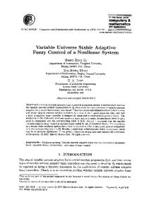
give the block diagram of a complete servomotor model. Inertias of load and motor are separated and the finite gear stiffness is taken into account in the diagram. Inserting nonlinearities of friction, amplifier current saturation, backlash and motor starting voltage completes the servomechanism model.4,12 Analytically, the DC-driven motor can be presented with equations
1 i' a = ----- ( – R a i a – Kθ' m + u ) La
(1)
1 θ'' m = ------ ( Kia – b m θ' m – T r – T fm sign ( θ' m ) ) , Jm
(2)
where ia is the current to the amplifier, θm the motor position in radians, La and Ra the inductance and resistance of the magnetizing circuit, K the gain factor of the motor, bm its damping factor, Jm the motor inertia, Tr the torque reduced from the load and Tfm the motor starting torque. These equations do not include the amplifier saturation, but in the simulations it is easy to limit the current ia. For numerical values, see appendix A. With backlash, the torque from load to motor can be written as
T v = 0 , if θ mr – θ l ≤ θ b
(3)
T v = K s ( θ mr – θ l – θ b ) sign ( θ mr – θ l ) , otherwise
(4)
where Ks is the gear stiffness factor and θl, θmr the load position and the motor position reduced to load, respectively. The gear ratio is introduced by equations
K Ra
+
1 s
1/La
u
+ -
K Saturation
1 s
1/Jm
Tfm
1 s
sign(x)
bm 1/n
1/n
Friction
position 1 s
1 s
disturbance
1/Jl
+
velocity
FIGURE 1.
Simulink block diagram for the open servomotor model.
+ +
+ -
Ks Backlash
θ θ mr = ----l. N
T r = NTv
(5)
N being the value of the gear ratio measured from the load. The friction model has three factors that have to be considered, namely static friction, kinetic friction and viscous friction. Static friction is the torque necessary to initiate motion from rest, kinetic friction is a friction component independent of the magnitude of the velocity and viscous friction is a component proportional to velocity. These components can be combined to give2
F(x) =
F C + D x' + ( F S – F C ) e
– b x'
sign ( x' ) .
(6)
In above equation, FC is the Coulomb friction parameter, FS coefficient for static friction, D the factor accounting for viscous friction and b is the parameter for static friction's range. In our model, static friction is improved by adding a constraint to friction for velocities practically equal to zero. Friction parameters are estimated from the inertia of the load. See appendix B for the implementation of friction in the simulation model. The Simulink diagram for the open servomotor system is shown in figure 1.
3.0 Fuzzy Controller Design The essential elements in designing a fuzzy controller include defining input and output variables, choosing fuzzification and defuzzification methods and above all, determining the rule-base of the controller. This is attempted first on pure heuristic basis. As the position servo is 'traditionally' controlled with a PD-controller, a PD-type fuzzy controller is chosen here too. Fuzzy controller is said to be PD-type if its inputs are error and change in error and output is the control signal. In this paper, triangular membership functions for the inputs and fuzzy singletons for the outputs are used. Minimum decomposition is chosen for fuzzy inference procedure and the center of gravity -method for defuzzification.8,9 1
NL
NM NS ZE PS PM
PL
de\e
NL
NM
NS
ZE
PS
PM
PL
NL
NX
NX
NX
NX
NS
ZE
PX
NM
NX
NX
NL
NL
NS
PS
PX
NS
NX
NL
NL
NM
PS
PS
PX
ZE
NX
NL
NL
ZE
PL
PL
PX
PS
NX
NS
NS
PM
PL
PL
PX
PM
NX
NS
PS
PL
PL
PX
PX
PL
NX
ZE
PS
PX
PX
PX
PX
0.5 0
Grade of membership
-1
-0.5
NL
0 Error
0.5
1
NM NS ZE PS PM
PL
1 0.5 0 -6
-4
-2
NX NL NM
NS
0 Change in error
ZE
2
4
6 x 10
PS
PM PL
-2
PX
1 0.5 0 -40
-20
0 Out
20
40
FIGURE 2. Membership functions for the PD-type fuzzy controller and the controller's rule-base presented as a fuzzy associative memory (FAM) -matrix.
On many references, it is stated that a quite small rule-base for the fuzzy controller should be selected in order to make the tuning procedure easier. In the nonlinear servomotor case the size of the rulebase becomes easily large, because the controller's behavior must change in a very nonlinear fashion in different situations. A rule-base of 7×7 rules proved to be simple enough to tune and good enough for accurate control. A fuzzy controller is relatively easy to tune to give approximately the wanted results. In order to meet the performance requirements, however, quite a lot experimenting and fine-tuning has to be done. Figure 2 shows the final membership functions and the rule-base of the controller. By plotting the control signal as a function of the inputs, the nonlinear properties of the fuzzy controller can easily be seen. This has been done in figure 3.
4.0 Simulation Results The goal in the tuning strategy is to obtain a fast response with no overshoot and with a negligible steady-state error. In addition, the controller is desired to compile with different size step responses. As is shown in figures 4-6, a single fixed rule-base fuzzy controller can be tuned for varying step sizes. The appropriate numerical integration method for this very nonlinear system is the Runge-Kutta fifth order method. Integration step size in Matlab is automatically varying, the tolerance was set at 0.001, minimum step size at 0.0001 and maximum step size at 0.001. 1 Simulations were run on SUN SPARCstation IPC. The fuzzy controller was implemented with sampling time of 0.01 seconds.
5.0 Other Controllers It is obvious that a traditional linear PID-controller is not an adequate solution to our servomotor control problem. This fact was clearly seen in several simulation experiments, too. Therefore, we will next try to tune a slightly better modification of the classical controller, namely the nonlinear PID-controller. Position (rad) 1 0.5
40 0 0
0.2
0.4
0.6
0.8
1
1.2
1.4
1.6
1.8
1.4
1.6
1.8
1.4
1.6
1.8
20
u
Control voltage (V)
0
40 20
-20
0 -20 0
-40
0.2
0.4
0.6
0.8
1
1.2
Amplifier current (A) 10
0.04 1
0.02 0 0
-0.02 -0.04 de
-0.06
-1 e
FIGURE 3. Control surface of the fuzzy controller, u as a function of e and de.
0 -10 0
0.2
0.4
0.6
0.8
1
1.2
FIGURE 4. Unit step response with fuzzy controller. 99 percent settling time ts is 1.12 sec and steadystate error e∞ is 3.03⋅10-4 radians.
A nonlinear PID controller is proposed by Shinskey.13 It is a controller with a continuous nonlinear function, the gain of which increases with amplitude. A modified nonlinear continuous PID-controller with filtering parameter N can be written as
TD s 1 C(s) = f( e )K P 1 + ------- + ------------------- , TI s TD ------s + 1 N
(7)
where f(|e|) is a suitable function. A function of the form
f( e ) = k + ( 1 – k ) e
(8)
with parameter k representing linearity is one possible choice, if e is restricted in the regions where f is positive.* Since there is little experience in tuning the above mentioned controllers, optimizing is one possible method to find appropriate values for the parameters of the nonlinear PID controller. Several criteria for optimizing the step response of a controller are known.7 The criterion chosen here is ITAE, Integral of Time multiplied by Absolute Error: M
J =
∫ t e(t) dt .
(9)
0
Time weighing in the loss function yields a shorter settling time. The Nelder-Mead simplex algorithm is used for optimizing the loss function. As figure 7 shows, a nonlinear PID-controller tuned for one step performs relatively well for a little larger and smaller step sizes. For large steps, however, the controller is quite sluggish and with small Position (rad)
Position (rad) 3
0.1
2 0.05 0 0
1 0.1
0.2
0.3
0.4
0.5
0.6
0.7
0.8
0.9
1
0 0
1
Control voltage (V) 50
50
0
0
-50 0
0.1
0.2
0.3
0.4
0.5
0.6
0.7
0.8
0.9
1
-50 0
1
Amplifier current (A) 10
0
0
0.1
0.2
0.3
0.4
0.5
0.6
3
4
5
2
3
4
5
4
5
Amplifier current (A)
10
-10 0
2
Control voltage (V)
0.7
0.8
0.9
FIGURE 5. Small step response. ts is 0.34 sec and e∞ is -8.93⋅10-4 rad.
1
-10 0
1
2
3
FIGURE 6. Large step response. ts is 2.36 sec and e∞ is 1.0⋅10-3 rad.
*: In 13, values of k are restricted to 0 < k ≤ 1.0, but we will need an increasing function with decreasing error and thus the largest allowed step size must be defined. One could also select a different f such that f is non-negative for all values of error.
steps there are problems with static friction, which results in significant position error until the integral part slowly corrects it. See appendix A for the nonlinear PID parameters.
6.0 Comparison of Robustness Next we will discuss the performance of the two controllers under external disturbance, load variations and motor parameter changes. Unit step is chosen here as the test reference signal. The external disturbance is modeled with a very strong, 50000 Nm step-wise torque applied to load (see figure 1). There is strong chattering in the control voltage of both controllers for a few tenths of seconds after the appearance of the disturbance. The fuzzy controller is able to hold the load position, but the nonlinear PID suffers from the disturbance. The eventual action of the integral part is so slow that it cannot be seen in figure 8. As the inertia of the load is increased, the fuzzy controller starts to give far too high control voltages, which makes its performance poor already at overload of forty percent. This is due to the strong control rules near the reference value to compensate backlash and static friction. With small increases in the load, the fuzzy controller is more accurate, while static friction affects strongly in the nonlinear PID case. Neither controller has major problems as the load is decreased. The fuzzy controller is faster, but with fuzzy control there is chattering in the control signal with very small values of load inertia. This is also due to the quite strong control signals near the reference value. 2 1
0.8
Position (rad)
Position (rad)
1.5
1
0.6
0.4
0.5 0.2
0 0
0.5
1
1.5 Time (sec)
2
2.5
3
FIGURE 7. A nonlinear PID-controller tuned for unit step.
0 0
0.5
1
1.5
2 Time (sec)
1
0.5
0.5
2
3
0 0
1
50 %
1
0.5
0.5
FIGURE 8.
1
4
2
3
2
3
60 %
1
0 0
3.5
40 %
1
1
3
FIGURE 8. A disturbance step applied at t=2 seconds. (Solid line: fuzzy controller, dashed: nonlinear PID)
20 %
0 0
2.5
2
3
0 0
1
Control results with increased load. (Solid line: fuzzy controller, dashed line: nonlinear PID)
Figure 10 shows effects of variations in the model parameters. The fuzzy controller is more accurate, but tends to become unstable with large parameter changes. The nonlinear PID does not have stability problems, but typically there is a long-lasting steady-state error until the integral part acts to correct it. One should remember that both controllers are designed to give fast responses and that this weakens their robustness. Controller tuning is always a compromise between tight performance criteria and robustness of the controller.15
7.0 Tuning Algorithm for Fuzzy Controller Finally, a new tuning algorithm for fuzzy controller is suggested. With our algorithm, it is possible to combine the desired properties of controllers tuned for several operating points to one fixed-rule-base fuzzy controller. The need of this algorithm arose from the fact that it is often easy to tune traditional controllers for one step size, but in the nonlinear case they may perform poorly for other step sizes.12,14 Our algorithm is the following: 1. Sample the step responses of the controllers tuned for different step sizes. At each sampling point, values of error, change in error and control signal are collected. 20 %
40 %
1
1
0.5
0.5
0 0
1
2
0 0
3
1
60 %
1
1
0.5
0.5
0 0
1
FIGURE 9.
2
3
2
3
90 %
2
0 0
3
1
Behavior of the controllers as the load is decreased. Backlash x 10
1
1 0.5 0 0
0.5
1
1.5
2
2.5
3
0.8
Position (rad)
Motor gain +50 % 1 0.5 0 0
0.5
1
1.5
2
2.5
3
0.6
0.4
Motor gain -25 % 1
0.2
0.5 0 0
0.5
1
1.5
2
2.5
FIGURE 10. Effects of parameter variations on control result.
3
0 0
0.2
0.4
0.6
0.8
1 1.2 Time (sec)
1.4
1.6
1.8
FIGURE 11. Responses of the fuzzy controller tuned with the optimization algorithm.
2
2. Determine the membership functions for e and ∆e. In our case, triangular MFs for inputs are used. 3. Select those rules who have sampled points in their support. Only these rules can be optimized.Variables that will be optimized are the places of output fuzzy singleton membership functions. 4. Optimize the rule-base ring by ring from the center point to the edge. In optimization, a numerical algorithm can be employed to minimize the error between fuzzy controller output and sampled output at each sampling point. Only those sampled data points that lie in the support of the rules of the corresponding rule-base ring are needed in evaluating the cost function. 5. For those rules that haven't been optimized a default value can be used. Default value may be e.g. zero or it may be computed from the control surface of one of the tuned controllers. The rule-base can often be mirrored in order to achieve same performance for negative steps. The optimization is done ring by ring in the rule-base because the control action near the equilibrium point must be more accurate than that with larger values of error. Control surface algorithm is tested in figures 12 and 11. Sampled step sizes were 0.5 and 1 radians, and 20 samples from each response were taken. The center points of the triangular membership functions for error were selected as [-1 -0.5 -0.25 0 0.25 0.5 1] and for change in error as [-0.03 -0.02 -0.01 0 0.01 0.02 0.03]. The results show that fuzzy controller can be tuned from sampled responses provided that there are enough samples and that the sampled responses are sufficiently near each other. Furthermore, for unit step the experimentally tuned controller has a little slower response but on the other hand it is more accurate than the fuzzy controller tuned with the surface optimization algorithm.
8.0 Conclusion
30 20 10 0 -10
20
u
u
We have simulated the nonlinear servomotor model, comparing fuzzy inference control and nonlinear PID control. Optimization was suggested as a possible way to determine the nonlinear PIDcontroller's parameters. Robustness experiments showed advantages and disadvantages of both controllers clearly. An approach to forming a nonlinear fuzzy controller's rule-base from training data was presented.
10 0 -10
1
2 0 -2
0 de
x 10
1
-2
30 20 10 0 -10
0 e
-1
-2
0 de
e
-1
-2
0 de
2
-2
x 10
40
u
u
e
-1
20 0 1 0 e
-1
-2
0 de
2
x 10
-2
1 0
FIGURE 12. The evolution of the control surface under the optimization algorithm.
2
-2
x 10
References [1] [2] [3] [4] [5] [6] [7] [8] [9] [10] [11] [12] [13] [14] [15]
“SIMULINK User's Guide”, The MathWorks Inc. 1992. B. Armstrong-Hélouvry, “Control of Machines with Friction”, Kluwer Academic 1991. C. Canudas de Wit, K. J. Åström, K. Braun, “Adaptive Friction Compensation in DC Motor Drives”, IEEE Int. Conf. on Robotics and Automation, San Francisco, USA, 1986. B. A. Chubb, “Modern Analytical Design of Instrument Servomechanisms”, Addison-Wesley 1967. H. Hashimoto, “Brushless Servo Motor Control Using Variable Structure Approach”, Proc. IEEE Industrial Applic. Soc. Annual Meeting, Sept. 1986. W. M. Humphrey, “Introduction to Servomechanism System Design”, Prentice-Hall 1973. T. Jussila, “Computational Issues of PID Controllers”, Ph. D. thesis, Tampere University of Technology 1992. B. Kosko, “Neural Networks and Fuzzy Systems”, Prentice-Hall 1992. C. C. Lee, “Fuzzy Logic in Control Systems: Fuzzy Logic Controller - Part I”, IEEE Trans. on Systems, Man and Cybernetics 2/1990. Y. F. Li, C. C. Lau, “Development of Fuzzy Algorithms for Servo Systems”, IEEE Int. Conf. on Robotics and Automation, Philadelphia, USA, April 24-29, 1988. J. Y. S. Luh, “Conventional Controller Design for Industrial Robots - A Tutorial”, IEEE Trans. on Systems, Man and Cybernetics, vol SMC-13, No 3, pp. 286-316. J. Riihilahti, H. N. Koivo, “Modeling and Adaptive Control of Electrical Servo”, Laboratory report, Tampere University of Technology 1990. F. G. Shinskey, “Process Control Systems, Application, Design and Tuning”, 3rd ed., McGraw-Hill 1988. N. K. Sinha, “Control Systems”, CBS College Publishing 1986. K. J. Åström, B. Wittenmark, “Computer Controlled Systems. Theory and Design”, Prentice-Hall 1991.
APPENDIX A.
APPENDIX B.
Numerical Values of the Servomotor Model
Friction model
b bm
function y = friction(u,Tr,Jl) Fc = Jl; Fs = 2*Jl; D = 0.2*Jl; b = 100; t1 = (Fc + D*abs(u))*sign(u); t2 = (Fs - Fc) * exp(-b*abs(u))*sign(u); if abs(u) > 0.001, y = t1 + t2; else y = min(abs(Tr),Fs)*sign(Tr); end
D Fc Fs Jl Jm iamax K Ks La n Ra Tfm
h N Kp Ti Td k
exponential friction factor motor damping coefficient
100 0.0007639 Nms/ rad2 viscose friction coefficient 40 Nms/rad Coulomb friction coefficient 200 Nm/rad maximal static friction 400 Nm/rad load inertia 200 kgm2/rad2 motor inertia 0.0012 kgm2/rad2 maximal amplifier current 8.5 A motor gain 0.488 Nm/A gear stiffness factor 1000000 Nm/rad inductance of magnetizing circuit 0.0004 H gear transmission 250 resistance of magnetizing circuit 1.6 Ω motor starting torque 0.1 Nm/rad backlash 0.005 rad sampling time filtering constant PID-controller gain integration time derivation time nonlinearity parameter
0.01 s 10 35.67 18.99 s 0.16 s 1.87