Fuzzy Global Attribute Oriented Induction Atanu Roy
Brendan M. Mumey
Department of Computer Science Montana State University - Bozeman Bozeman, MT, 59715
[email protected]
Department of Computer Science Montana State University - Bozeman Bozeman, MT, 59715
[email protected]
Abstract— Attribute-oriented induction is a useful technique that summarizes data of relatively-low values with higher-level concepts. In a large database, it is always beneficial to describe generalized knowledge, rather than lower levels of abstraction. In this paper we modify the concept of AOI and we apply it on a fuzzy relational database. Following the concept proposed by Chen et al. [1] to mine generalized knowledge from a relational database; we propose two techniques which can successfully handle multi-valued attributes from a fuzzy relational database. Keywords – attribute oriented induction; fuzzy relational databases; levels of abstraction; proximity functions.
I.
INTRODUCTION
Most of the transactional or warehouse databases that we handle contains huge amount of data. Performing data mining analysis on these databases is very tough because of the extensive volume of data. Thus, we need some techniques to convert the raw data into some condensed form, so that data mining analysis can be done on it [8-9]. Attribute-Oriented Induction (AOI) is one such technique which converts massive amounts of data in a relational database using data mining techniques to generalized knowledge. It is an iterative process in which similar data items are grouped together to provide the user with a more generalized view of data. In this technique, the data is compressed and presented in a more generalized relation, which conveys a concise summary of the total knowledge. Since data mining applications are computationally intensive, thus having a large dataset as its input is not advisable. AOI provides us with the tool to prune the uninteresting parts of the database. Moreover if the end user is only concerned with higher level of abstractions, it is highly inefficient to use the whole database for knowledge discovery. The pre-processing of data using AOI is done for each attribute in the database. There are some attributes (e.g. SSN, any kind of ID) in a database which does not contribute much to the global generalized knowledge. These attributes are those which have a large set of distinct values and there is (1) either no generalization operator for the relation (e.g. absence of concept hierarchy) or (2) its higher level concepts are expressed in terms of some other attributes’ hierarchy [10]. Through the process of attribute removal, these attributes are identified and are removed before AOI is applied. Separate attribute hierarchies are applied for each attribute as a part of Paper to be submitted for review on April 23, 2010. This work was supported by Department of Computer Science, Montana State University.
the attribute generalization process. The attribute hierarchy which is an input to the AOI algorithm is a supplementary piece of knowledge that is provided by the experts. The AOI algorithm uses these attribute hierarchies to generate the generalized knowledge. In the subsequent sections we will discuss a variant of this approach proposed by Chen et. al. [1] and how we generalize the concept to derive knowledge even from fuzzy relational databases. The concept of relational databases proposed by Codd in 1970 [1] is based on set theory and the theory of relation. Fuzzy set theory proposed by Zadeh [5] is a deviation from the original set theory. Buckles, et al. [4] combined the concept of relational databases and Zadeh’s fuzzy set theory to propose a database model which can handle multi-valued attributes. A fuzzy relational database essentially contradicts the first normal form which is an integral feature of a relational database. Instead of having atomic values, a fuzzy relational database can have more than one value for an attribute in a tuple. Thus a fuzzy relational database is a generalization of classical relational database. It is formally defined as a set of relations where each relation is a set of tuples. ti represents the ith tuple. It has the form (di1, di2, ..., dim), where dij represents the jth attribute of the ith tuple. In a relational database, each component, dij, of the tuple is a single component which is an element of the domain Dj, i.e., dij Dj. But in the fuzzy relational database, the above mentioned constraint is not satisfied, that is the tuple components are not confined to single elements drawn from scalar domain, instead dij Dj (dij ≠ Φ). An example of a finite scalar domain is {Audi, BMW, Porsche} and an example of a continuous scalar domain can be Price {VExpensive (45000 - 54999), ExtremelyExpensive (55000 - 200000)}, then the domain values of a particular tuple may be a single value or a sequence of values. Table 1: Snapshot from a fuzzy database Manufacturer Model EngineDisplacement Price {Audi, BMW} {Sports {4500} {50000 Car} 60000} The remainder of the paper is organized as follows. Section II provides a list of the related works. Section III defines the important terms and states the problem formally. Section IV discusses GAOI algorithm in brief. Section V is devoted to the discussion of our naïve algorithm. Section VI is devoted to experimental results. We conclude our research and put forth
our future works in Section VII & VIII. Moreover our new scaled fuzzy GAOI is put forth in Section IX. II.
RELATED WORKS
The concept of Attribute-Oriented Induction was proposed in 1991 [11] by Cai, et. al. The generation of each attribute is associated with an attribute hierarchy. The attribute hierarchies represent necessary background knowledge which controls the generalization process. Different concepts are often organized based upon levels in an attribute hierarchy. The concepts range from the single, most generalized root concept, to the most specific concepts corresponding to the specific values of attributes database [12, 13]. Much research has gone into the extension of AOI originally proposed by Cai et al. Carter et al. [14] proposed more efficient methods of AOI. Angryk et al. [6] combined fuzzy sets and AOI. They proposed an approach for AOI to handle fuzzy relational databases. Some researchers [15] applied AOI in complex databases to generalize it. But the extension we are interested in was proposed recently (2010) by Chen et al. In this approach the researchers took a fundamentally different approach from what has already been done. The researchers were able to mine multiplelevels and employ multiple minimum supports to generate interesting tuples. The approach proposed by [1] expects the input to be a relational database following Codd’s first normal form. In this work we propose two algorithms which have the ability to handle fuzzy relational databases. At first we propose a naïve algorithm which creates the output relation in a relatively short amount of time. This approach is not computationally expensive and can be used with complex fuzzy relational databases. The second approach that we propose is a computationally expensive one. But the quality of knowledge discovered is superior from its naïve counterpart. III.
BACKGROUND
In this section we define the terms that we will be using throughout the paper. Moreover we will also provide a formal statement of the problem that we have tackled in this research. For the rest of the paper we will reference the sample dataset of Appendix A. In order to save space all the attribute hierarchies are provided in Appendix B. Let A = {at1, at2, at3, …, atn} be a set of attributes for the tth tuple where ati Di (ith domain), which corresponds to a corresponding attribute hierarchy Ti. A value in the attribute hierarchy is called a node. Based on these notations we define a few important terms. A. Definitions 1) Value :A value vk, i denotes it as the kth element of Tith tree, where the sequence of nodes are numbered in some tree traversal order.
Fig 1. Attribute Hierarchy for T3 Thus if a car or a light truck has an engine displacement of 3500, then it would be represented as v8, 3. But if the displacement attribute of a vehicle is a fuzzy attribute, then it may be defined as a range. For example if the vehicle has an engine displacement between 3500 – 4250, then we would represent the data as v8, 3, v9, 3. 2) Valuesets: A valueset l = { , , , ,…, , } where r ≤ no. of attributes is a non-empty set of values, where no two values in the set belongs to the same attribute. A valueset with k values is known as a k-valueset. 3) Level: lvl(vk,i) denotes the level of the value vk,i in the attribute hierarchy Ti. For example lvl(v9,3)=2 and lvl(v3,3)= 1. 4) Cover: cov(l) of a valueset l = { , , , ,…, , } is defined as the union of all the tuples which contains either the vkn for attribute ir or any descendents of vkn in the attribute hierarchy of ir. 5) Support: sup(l) of valueset l is defined as cov(l) over the total number of tuples in the database (D). |c
| |D|
(1)
6) Minimum level support: Each level in an attribute hierarchy is has a minimum support provided by the user. Each value in the valueset will have a minimum support based on its level. The attribute which has the lowest minimum support is attributed to be the MLS(l) of the whole valueset l. 7) Frequent: A valueset l is considered to be frequent iff sup(l) ≥ MLS(l). Without loss of generality tuple t is considered to be frequent iff sup(t) ≥ MLS(t). 8) Potentially Frequent: A valueset l is considered to be potentially frequent iff sup(l) ≥ MIN(l), where MIN(l) is defined as the MLS of the lowest level of the attribute hierarchy. Without loss of generality tuple t is considered to be potentially frequent iff sup(t) ≥ MIN(t). 9) Interest: Not all tuples which are frequent contribute to the global generalized knowledge. Thus the concept of interest I(t) of a tuple t with r attributes is defined as ∑
sup v
(2) ,
A tuple with a value I(t) ≥ δ is considered interesting where δ is a user-defined constant ≥ 1. B. Problem Statement: Given a fuzzy relational database D, and a set of MLS thresholds for each attribute hierarchy, we have to find all the interesting tuples. IV.
GLOBAL ATTRIBUTE-ORIENTED INDUCTION
In this section we will briefly discuss about the Global AOI (GAOI) algorithm proposed by [1]. The GAOI algorithm is a remedy to the drawbacks of the traditional AOI algorithm. In this technique, the researchers employ multiple minimum level support concept and multiple-level mining to generate global general knowledge. The inputs to the algorithm are (1) a relational database D; (2) the attribute hierarchies of the task relevant attributes; (3) a set of MLS threshold; (4) an interest measure. The output from the algorithm is all the “interesting generalized” tuples from D. GAOI is essentially a four-step algorithm. In the first part of the algorithm the task-relevant tuples are chosen and encoded. The encoding is done in order to save memory and it also ensures an ease of calculations. The encoding process will be further discussed in the next section. In the next step, the frequent generalized tuples (FGT) are discovered. The algorithm for generation of FGT is an extension of method for mining multiple level association rules [16] and uses Liu et al.’s [17] concept of multiple minimum support. This is an iterative process where all the 1-valuesets from D are extracted. Next the potentially frequent (P1) tuples and frequent tuples (F1) are identified. The 2-valuesets are generated using F1 and P1. After the generation of 2-valuesets the higher k-valuesets (k > 2) are generated iteratively from the (k - 1)-valuesets. As discussed all the tuples generated by the FGT are not interesting to the user. Thus the output of the FGT algorithm is pruned according to interest measures of the tuple. The last step of the algorithm is to decode the interesting to original values according to the attribute hierarchies and present it to the user. V.
NAÏVE FUZZY GAOI
We start our discussion of the naïve version of the algorithm which proposes an approach to handle fuzzy data. The proposed algorithm is based on the GAOI algorithm discussed in the last section, but our algorithm has the capability to derive knowledge even from fuzzy relational tuples. The input to naïve fuzzy GAOI algorithm is (1) a fuzzy relational database; (2) a set of proximity relations and a set of attribute hierarchies; (3) a set of MLS threshold; (4) an interest
measure threshold. Table 2 contains a brief description of the algorithm with the major steps involved. Table 2: Snapshot of the Naïve Fuzzy GAOI Algorithm Algorithm: Naïve Fuzzy GAOI Input: (1) a fuzzy relational database; (2) a set of proximity relations and a set of attribute hierarchies; (3) a set of MLS threshold; (4) an interest measure threshold. Output: Interesting tuples learned from the fuzzy relational tuples Method: 1. Identify, collect and convert multi-valued attributes. 2. Encode all the task-relevant tuples. 3. Discover the frequent generalized tuples. 4. Prune the uninteresting tuples. 5. Decode and output the final set of tuples. A. Identify, collect and convert the fuzzy tuples The first step for the Naïve Fuzzy GAOI algorithm is to identify the multi-valued attributes in the database. As already discussed in the previous section, a fuzzy attribute does not conform to Codd’s 1NF [2]. Thus any attribute of a tuple which contains multi-valued leaf attributes from a particular attribute hierarchy is identified as a fuzzy tuple. When a multi-valued attribute is identified, the data has to be converted to Codd’s 1NF. We search the relevant attribute hierarchy and replace the multi-valued attributes with the lowest node in the hierarchy that has all the values as direct or indirect descendants. Example 1: In Appendix A, the “Model” attribute of the fourth tuple contains multiple leaf attribute values: “FullsizeCar, SportyCar”. Multiple values for the same attribute has to be replaced by a single value. Thus, the lowest nodes in the “Model” attribute hierarchy that has both “FullsizeCar” and “SportyCar” as a direct or an indirect offspring is the node “Car” which is illustrated in Fig. 2. In the same way the model attribute of the 16th tuple is converted from “CompactPickUp, FullsizePickUp”, into “PickUp”. The conversion of continuous data using this algorithm requires an explanation. Instead of having two distinct values, as we found in the case of the categorical attributes, continuous data is expected to be a range of values. Thus, the algorithm needs to identify the range and correctly convert the data into categorical format. This refers to fact that our algorithm needs to correctly identify the node farthest down in the tree whose range encompasses the data range. Example 2: In Appendix A, the “Price” attribute of the fourth tuple contains a range of prices “18000-24990”, instead of a distinct price. Thus the node farthest in the tree that encompasses this range is “Economic”. So, the algorithm replaces the continuous range with a discrete categorical value. Thus our algorithm can eliminate the multi-valued attributes that is expected to be present in a fuzzy relational database.
Fig. 2. Replacement of fuzzy data with precise data. B. Encode all the task-relevant tuples Next we consider the output of the intermediate database of Step 1 as the input to this step. In this step we encode every task-relevant attribute into a generalized identifier (GID). The GID is applied on the basis of attribute hierarchy traversal. A GID is an integer that contains the route information for an attribute value in the corresponding attribute hierarchy. Example 3: In the relational database, the second attribute is model. We will take a random precise value from the table and encode it. Suppose the attribute value is “FullsizeCar”. Since model is the second attribute thus
Fig 3. Attribute Hierarchy showing encoded numbers We start the encoding process with 2. In the next level we move to “car” and thus we append a 1 after 2. Next we move on to “General Car” and next to “FullsizeCar”. Thus the total route is 2112. We encode “FullsizeCar” as 2112. Next we handle fuzzy data or values from a higher level of abstraction. Suppose we encounter a multi-valued attribute “CompactCar, FullsizeCar”. By the first step of our algorithm it will get replaced by “General Car”. Since “General Car” is not a precise data, thus the encoding process is a bit different. The process until we find “General Car”, which gives us a result of “211” is same. Since all the encoded formats should have same number of letters, we append a 0 at the end to convert it to “2110”. Thus if we encounter a value like “Light Truck”, the encoded value will be “2200”. At the highest abstraction level, the encoding value is “000”. Since the attribute engine displacement has three levels of abstraction instead of four, we append a 0 at the end for the precise values of that attribute.
C. Discover the frequent generalized tuples The generation of FGT is an extension of the algorithm proposed by Chen et al [1]. In this algorithm as already discussed we find out the 1-valuesets and divide into P1 and F1. Next we generate the k-valuesets in an iterative process. The first iteration is for creating the 2-valueset which is generated by combining P1 and F1. Next the k-valuesets are created by combining the (k-1)-valuesets. The algorithm for the FGT algorithm is provided in Table 2. Table 3: FGT Algorithm FGT: For discovering the frequent generalized tuples Input: (1) The hierarchical-information encoded table. (2) The set of MLS thresholds. Output: A set of frequent general tuples G. Algorithm: FGT(T, MLS) { 1. C1 = scan(T) 2. P1 = {v| v ε C1: supp(v) ≥ MIN(v) } 3. F1 = {p| p ε P1: supp(p) ≥ MLS(lvl(v)) } 4. for(k = 2; k ≤ |attr|; k++) { 5. //|attr| = no. of task-relevant attributes 6. if(k == 2) 7. F2 = 2-valuesetsgen(F1, P1) 8. else 9. Fk = k-valuesetsgen(Fk-1) 10. } 11. G = } Example 4: Consider T as shown in Table 3. Let us assume that the MLS for different levels MLS(1) = 35%, MLS(2) = 25%, MLS(3) = 15%. Thus MIN for the table would be 15%. Since the database has 20 tuples, thus any 1valueset having support count of 3 or more will be considered potentially frequent. Table 4: Snapshot of 1-valset table sup
val
Cover
freq
pfreq
0.45
1100
1 3 4 6 13 14 15 16 18
Y
Y
0.25
1110
1 13 14 15 18
Y
Y
0.15
1111
1 15 18
Y
Y
0.05
1112
13
N
N
0.05
1113
14
N
N
0.20
1120
3 4 6 16
N
Y
… 0.50
… 2200
… 2 5 8 11 12 14 16 17 19 20
… Y
… Y
0.25
2210
2 8 11 12 14
Y
Y
0.15
2211
8 11 12
Y
Y
0.10
2212
2 14
N
N
Property 1: One of the most important concepts proposed by [1] is the concept of “Level Sorted Order”. A valueset l = { , , … , } satisfies the property if MLS(lvl(v1)) ≤ MLS(lvl(v2)) ≤ … ≤ MLS(lvl(vk)). For example, a valueset having the value 1200, 3210, 4000, 2132 is level sorted only if the values are ordered in 2132, 3210, 1200, 4000. Lemma 1: “Level Closure Property” [1] states that if a kvalueset is level sorted and is frequent, then all of its level sorted (k-1)-valuesets are frequent. Based on the level closure property, the 2-valuesetgen function takes two arguments F1 and P1. The algorithm is as follows Table 5: 2-valsetgen algorithm. 2-valuesetsgen: Generation of 2-valuesets. Input: (1)The frequent and potentially frequent 1-valuesets Output: All frequent 2-valuesets Algorithm: 2-valuesetsgen (F1, P1) { 1. for each value v ε F1 do 2. for each value p ε P1 do 3. if(sup(p) ≥ MLS(lvl(v)) and attr(p) != attr(v)){ 4. cov(v, p) = cov(v) ∩ cov(p) 5. sup(v, p) = |cov(v, p)|/ |D| 6. if(sup(v, p) ≥ MLS(lvl(v))) 7. insert (v, p) in F2 8. } } Example 5: Suppose we have v = 1110 which has a support of 25% and p = 4220 has a support of 15%. If we try to create a 2-valueset from them, it will fail since sup(4220) < MLS(lvl(1110)) = 25%. But 1110 will create a frequent 2valueset with 3100 which has a support of 30% since sup(3100) > MLS(lvl(1110)) = 25% and cov(1110, 3100) = {1 13 14 15 18} which has a support of > MLS(lvl(1110)) = 25%. Once the 2-valueset table is created, we are only left with creating the rest of the valuesets up to k-valueset. This process can achieved with the help of a single algorithm which creates k-valueset from (k-1)-valuesets. In this algorithm two valuesets from the Fk-1 table is checked to see whether the first k-2 values of the two valuesets match. And if they match and the (k-1)th values belong to different attributes, we calculate the support of the intersection of the cover of both. If the support is more than the MLS threshold of the valueset, we include the value in the Fk table. Example 6: Let F3 be {, }. Since u.val1 = v.val1 = 4211 and u.val2 = v.val2 = 3310 and attr(2230) = 2 != attr(1300) = 1, thus we calculate the intersection of their covers. {(5, 17, 19) ∩ (2, 5, 17, 19)} = {{(5, 17, 19)}. sup(cov{}) ≥ MLS(lvl(4211)) . Thus we insert in F4.
The last step of FGT algorithm unions all the k-valuesets (k > 1), and dumps the generalized tuples into G. For those valuesets where k < |attrno| we insert “any” to convert the tuple into a |attrno|-valueset tuple. Table 6: k-valsetgen algorithm. K-valuesetsgen: Generation of k-valuesets. Input: (1)k-1 valueset Output: All frequent k-valuesets Algorithm: //attr(x) returns the attribute no. of x k-valuesetsgen (Fk-1) { 1. for(k=3; k≤|attrno|; k++){ 2. for each value v ε Fk-1 do 3. for each value u ε Fk-1 where u.ID > v.ID do 4. if(v.val1 = u.val1 & … & v.valk-2 = u.valk-2 & attr(vk-1) != attr(uk-1)){ 5. cov(v, u) = cov(v) ∩ cov(u) 6. sup(v, u) = |cov(v, u)|/ |D| 7. if(sup(v, u) ≥ MLS(lvl(u.val1))) 8. insert (v, u) in Fk 9. } 10. } } Example 7: For the tuple in F3 {(2100, 4100, 1100)} we insert an “any” at the end and thus eventually it gets converted to {(2100, 4100, 1100, 3000)}. D. Prune the uninteresting tuples In this step we prune the un-interesting tuples before presenting it to the user. We use (2) to compute interest measure of a tuple in G. If the tuple fails to cross the userdefined interest threshold (δ), we delete the tuple from the output relation. Example 8: For the tuple presented in example 7, we will calculate the interest. Since the cover of the tuple is {1 3 4 6 13 15 18}, its interest measure is 35%/(50% x 45% x 45% x 100%) = 3.46 and δ = 3. Since I(g) > δ, thus we preserve this tuple and present this to the user. E. Decode and output the final set of tuples The last part of the algorithm deals with decoding the result using the attribute hierarchy. Example 9: If we are to continue with the previous example, the final tuple would look like {Asia, Car, any, Low Price} VI.
EXPERIMENTS & RESULTS
In order to evaluate the performance of our algorithm, we conducted a number of experiments primarily using the dataset from Appendix A on the following system: •
Dell OPTIPLEX GX620
•
• •
Pentium 4 CPU , 3.4 GHz , FSB 800 MHz, 1 core 2 GB of RAM , 533 MHz OS – Windows XP SP3 , 32 bit
All algorithms were implemented using Java programming with the help of JDBC driver for the database connection to My SQL Server 5.0.77 – 3.el5. There are four attributes (Manufacturer, Model, Engine Displacement, Price) and 20 tuples in the database. Throughout our experiments we keep the number the MLS of the levels as MLS(1) = 35%, MLS(2) = 25% and MLS(3) = 15%. Moreover in the experiments described below, we have compared our naïve fuzzy GAOI approach with a grabfirst approach. “Grab first” can be described as an approach where if we encounter a multi-valued attribute, we grab the first descriptor and discard the others to convert the tuple into Codd’s first normal form. Thus this approach converts the fuzzy database into a relational database without changing the tuple count. We present the results of our experiments. A. RunTime Test: In this performance evaluation, we test the average run time of our algorithm against the grab-first algorithm. We calculate the run time against the number of attributes. In the 2 attribute scenario we use “Manufacturer” and “Model”, whereas in the 3 attribute scenario we use “Manufacturer”, “Model” and “Price”. The results are presented in Fig. 5. This performance test clearly shows the fact that as the number of attributes increase, so is the difference between the two approaches increase. Since, in this expermiment the naïve fuzzy algorithms has to identify more fuzzy tuples and thus have to convert them to higher abstraction levels, the time difference between the two increases.
160 140 120 100 80 60 40 20 0
grab‐first
Naïve fuzzy GAOI
B. Quantity of Knowledge: Next we test the grab-first algorithm and naïve fuzzy algorithm with respect to the number of interesting tuples they generate. This test quantifies the amount of knowledge that we are losing due to the over-generalization of the naïve fuzzy algorithm. We test using different interest measures and check for the number of interesting tuples presented to the user. 300
Naïve fuzzy GAOI grab‐first
250 200 150 100 50 0 1
2
3
4
5
6
7
8
9
Fig 5. Interest measure vs no. of generalized tuples As expected due to the higher levels of abstraction, which naïve fuzzy GAOI algorithm generates for fuzzy tuples, it is losing on the number of generalized tuples considerably. VII. CONCLUSIONS In this research we have successfully shown that our approach can derive generalized knowledge from fuzzy relational databases. Our concept is based on multiple-level mining techniques, multiple minimum level support concepts and Zadeh’s fuzzy set theory concepts. The results show that the proposed method is efficient and can be scaled for fuzzy relational databases. VIII. FUTURE WORK
1
2
Fig. 4. No. of attribute vs Run Time
3
There are a lot of possible directions for future work. One such direction can be to calculate the possibility of the occurrence of a particular value in a multi-valued attribute and calculate real support instead of having an integer support. We call this algorithm “Scaled Fuzzy GAOI”. Since we have not yet tested this approach, thus we propose this approach in our future work section.
Sports Car Sports Car Sporty Car Compact Van Fullsize Van Compact PickUp Fullsize PickUp IX.
Table 7: α-Proximity table for attribute model Sporty Compact Fullsize Compact Car Van Van PickUp
Fullsize Pick Up
1
0.8
0
0
0
0
0.8
1
0
0
0
0
0
0
1
0.8
0.5
0.5
0
0
0.8
1
0.5
0.5
0
0
0.5
0.5
1
0.8
0
0
0.5
0.5
0.8
1
SCALED FUZZY GAOI
In the scaled fuzzy GAOI approach, the approach towards handling fuzzy data changes drastically from its naïve counterpart. In the naïve approach whenever we encounter a fuzzy data, we move a certain level up in our attribute hierarchy. The elegance of the solution is to handle fuzzy data without using a computationally expensive framework. But on the other hand, in the naïve approach we were overgeneralizing the problem and missing out on the quality of the knowledge produced. A. Background Knowledge The original characteristics of fuzzy proximity relations as proposed by Shenoi et al. [18] were reflexive and symmetric. But, to introduce the idea of transitivity via sequence of similarities, the researchers [19] used Tamura chains [20]. Thus the α-proximity relations in fuzzy relational databases have the following characteristics. If P is a proximity relation on domain Dj and the values of α ε [0, 1], then two elements x, z ε Dj are α-similar (denoted by xPαz) iff P(x, z) ≥ α and are said to be αproximate or there exists a sequence y1, y2, …, ym ε Dj : xPαy1Pαy2Pα… Pαym Pαz. To discuss the proximity relations, let us use a modified version of the Model attribute hierarchy as represented in Appendix B. The proximity table is provided in the Appendix C. From table 5, we can conclude that the partition tree will be as follows B. Algorithm The input to the scaled fuzzy GAOI algorithm includes (1) a fuzzy relational database; (2) a set of proximity relations and a set of attribute hierarchies; (3) a set of MLS threshold; (4) an interest measure threshold; and (5) a fuzzy proximity table for every multi-valued attribute. The algorithm starts its run scanning over the fuzzy relational database. It first searches for the distinct occurrences of the task-relevant attributes and calculate the count and cover of each. Next the algorithm scans the
intermediate table and identifies the multi-valued attributes. Our solution is based upon partial vote propagation approach proposed by Angryk and Petry [4]. In this approach we consider a single database tuple as one vote. Now fractions of vote are assigned to the fuzzy data values to represent each of the originally inserted values.
Fig 6. Partition tree of the attribute Model The naïve way of splitting the vote is to divide the vote equally among all the inserted descriptors. This approach fails to capture the real-life dependencies which are represented by the fuzzy proximity table. Instead we use the partial vote propagation approach proposed by [4]. In this approach the researchers does a recursive preorder traversal of the partition tree. The tree is searched from the root until the particular descriptor is reached in the tree. Example 10: An example of this can be a tuple which is of the form {, , , }. The attributes in this tuple follow the standard pattern that we followed throughout our discussion. The attribute model is the multivalued attribute in this tuple. The output of the algorithm provides us with the similarity levels is as follows
Table 8: Subsets of similarities according to α-proximity tables and partition tree
[3]
Output {SportsCar, CompactVan, FullsizeVan} | 0.0
Comments Stored
[4]
{SportsCar} | 0.5
Stored
{SportsCar} | 0.8
Updated
{SportsCar} | 1.0
Updated
{CompactVan, FullsizeVan} | 0.5
Stored
{CompactVan, FullsizeVan} | 0.8
Updated
{CompactVan} | 1.0
Stored
{FullsizeVanVan} | 1.0
Stored
[7]
[8]
Next we apply summarization values to each individual descriptor. Since “SportsCar” was reported twice, thus its summarization value is (1.0 + 0.0) = 1.0 Similarly the summarization values of the other two descriptors are as follows: CompactVan {1.0 + 0.8 + 0.0} = 1.8 FullsizeVan {1.0 + 0.8 + 0.0} = 1.8 Now we calculate the partial vote for each by normalizing the values of each. SportsCar (1.0/ (1 +1.8 + 1.8)) = 0.22 CompactVan (1.8/ (1 +1.8 + 1.8)) = 0.39 FullsizeVan (1.8/ (1 +1.8 + 1.8)) = 0.39 Once we calculate the partial vote of each of the descriptor we multiply the support of tuple with the partial vote of each of the values and create that many tuples in the next intermediate database. Thus instead of having integer supports, we will be left with fractional supports for each tuple that has been created. From this intermediate database 1-valuesets will be calculated and the rest of process will be followed as we did for our naïve fuzzy approach Example 11: For the tuple from the previous example if we have a support count of 4, we will create 3 tuples in the intermediate database with fractional support as illustrated in Table 7. Table 9: Snapshot of intermediate database Engine Manufact Model Displac Price urer ement
Support
SportsCar
2700
25230
0.88
Chevrolet
ComapctVan
2700
25230
1.56
Chevrolet
FullsizeVan
2700
25230
1.56
[1]
[2]
[9]
[10] [11]
[12]
[13]
[14]
[15]
[16]
[17]
[18]
Chevrolet
X.
[5] [6]
REFERENCES
Y. L. Chen, Y. Y. Wu, and R. I. Chang, “From data to global generalized knowledge”, Journal of Knowledge and Information Systems. 2010 in press. F.E.Codd, "A relational model of data for large shared data banks", Communications of the ACM, 13(6), 1970, pp. 377-387.
[19]
[20]
De S. K., Biswas R, and Roy A. R. (2001), “On extended fuzzy relational database model with proximity relations”, Fuzzy Sets and Systems, 117 (2), pp. 195-201. Buckles B.P. and Petry F.E. (1982), “A fuzzy representation of data for relational databases”, Fuzzy Sets and Systems 7(3) pp. 213 – 226. L.A. Zadeh, Fuzzy sets, Inform. and Control 8 (1965) 338-353. R. Angryk, F. Petry, Knowledge discovery in Fuzzy Databases Using Attribute-Oriented Induction, in: T.Y. Lin, S. Ohsuga, C.J. Liau, X. Hu (Eds.), Foundations and Novel Approaches in Data Mining, Series: Studies in Computational Intelligence, Vol. 9, SpringerVerlag, 2006, X, 376 p. 60 illus., pp. 169-196. J. Han and Y. Fu. Exploration of the Power of Attribute-Oriented Induction in Data Mining. In U. M. Fayyad, G. Piatetsky-Shapiro, P. Smyth, and R. Uthurusamy, editors, Advances in Knowledge Discovery and Data Mining. AAAI Press/MIT Press, M. Goebel and L. Gruenwald, A survey of data mining and knowledge discovery survey tools. ACM SIGKDD Explorations Newsletter 1(1), (1999), pp. 20-33 A. Feelders, H. Daniels and M. Holsheimer, Methodological and practical aspects of data mining, Information & Management 37, 2000, pp. 271 – 281. J. Han and M. Kamber, Data Mining: Concepts and Techniques, 2001 Morgan Kaufmann Publishers, USA. Y. Cai, N. Cercone, and J. Han, Attribute-oriented induction in relational databases.In G. Piatetsky-Shapiro& W. J. Frawley (Eds.), Knowledge discovery in databases, 1991 (pp. 2 13-228). Cambridge, MA: The MIT Press. J. Han, Y. Cai, and N. Cercone. Knowledge discovery in databases: an at,tribute-oriented approach. In Proceedings of the 18th International Conference on Very Large Data Bases, pages 547-559, Vancouver, Canada, 23-27, August 1992. Y. L. Chen, and C. C. Shen, "Mining Generalized Knowledge from Ordered Data through Attribute-Oriented Induction Techniques", European Journal of Operational Research, 2005, Vol. 166 No. 1, pp. 221-245. Carter, C.L. and Hamilton, H.J. (1998), "Efficient Attribute-Oriented Generalization for Knowledge Discovery from Large Databases", IEEE Transactions on Knowledge and Data Engineering, Vol. 10 No. 2, pp. 193-208. Knorr, E.M. and Ng, R.T. 1996. "Extraction of Spatial Proximity Patterns by Concept Generalization." In Proc. 2nd Int. Conf. on Knowledge Discovery and Data Mining (KDD). Han, J. and Fu, Y. (1999), "Mining Multiple-Level Association Rules in Large Databases", IEEE Transactions on Knowledge and Data Engineering, Vol. 11 No. 5, pp. 798-805. Liu, B., Hsu, W. and Ma, Y. (1999), "Mining Association Rules with Multiple Minimum Supports", Proceedings of the fifth ACM SIGKDD international conference on Knowledge discovery and data mining, pp. 337-341. S. Shenoi, A. Melton, Proximity relations in fuzzy relational database model. International Journal of Fuzzy Sets and Systems, 1989, 31(3), pp. 285-296. S. Shenoi, A. Melton, Fuzzy relations and fuzzy relational databases, Intenational Journal of Computers and Mathematics with Applications 1991, 21 (11/12), pp. 129-138. S. Tamiura, S. Higuchi, K. Tanaka, Pattern classification based on fuzzy relations, IEEE Transaction on Systems, Man, and Cybernatics 1971, 1(1), pp. 61-66.
XI. ID 1 2 3 4 5 6 7 8 9 10 11 12 13 14 15 16 17 18 19 20
Manufacturer Kia
Chevrolet Chrysler Toyota Nissan Hyundai Honda Chrysler Nissan BMW Porsche Fiat Chevrolet Porsche Ferrari Ford Chevrolet Daewoo Kia Mazda Hyundai BMW Dodge Kia Mazda Chrysler Kia Dodge Novabus Chevrolet
APPENDIX A: FUZZY DATABASE TABLE
Model CompactCar SportsCar FullsizeVan CompactCar FullsizeCar SportyCar CompactSUV CompactPickUp Compact Van FullsizeCar SportsCar SportyCar CompactCar CompactVan SportsCar SportsCar SportyCar CompactVan FullsizeVan CompactVan FullsizeVan FullsizeCar FullsizeVan CompactCar SportsCar FullsizePickUp CompactPickUp FullsizePickUp CompactSUV CompactCar SportsCar FullsizeCar CompactSUV FullsizeSUV
Engine Displacement 1500 - 1600 3500 - 4250 1600 - 2000 4001 - 6000 3200 - 3500 2500 - 3200 4500 2700 4000 6000 2500 2700 - 3050 1600 1600 1600 3200 3200 - 4500 1300 1500 - 4000 4700
XII. APPENDIX B: ATTRIBUTE HIERARCHIES
Price 9000 - 12250 26900 14950 18000-24990 22000 - 28635 24000 52500 - 60000 25230 54000 - 59100 186925 25000 25230 - 36000 23980 20343 9000 - 12250 15535 28635 9998 - 15000 27335 - 36000 32905
XIII. APPENDIX C: PROXIMITY RELATION FOR MODIFIED MODEL ATTRIBUTE Attribute Hierarchies for all the attributes. Sports Car Sports Car Sporty Car Compact Van Fullsize Van Compact PickUp Fullsize PickUp
Sporty Car
Compact Van
Fullsize Van
Compact PickUp
Fullsize Pick Up
1
0.8
0
0
0
0
0.8
1
0
0
0
0
0
0
1
0.8
0.5
0.5
0
0
0.8
1
0.5
0.5
0
0
0.5
0.5
1
0.8
0
0
0.5
0.5
0.8
1