This characteristic enables the search for an entire set of Pareto optimal solutions, at ... In mathematical notation, a multi-objective optimization problem can be ...
Fuzzy Logic Controlled Multi-Objective Differential Evolution Feng Xue* *
Arthur C. Sandersonξ Piero P. Bonissone* Robert J. Gravesξ
General Electric Global Research, One Research Circle, Niskayuna, NY 12309, USA ξ Rensselaer Polytechnic Institute, 110 8th St, Troy, NY 12180, USA
Abstract- In recent years, multi-objective evolutionary algorithms (MOEA) have generated a large research interest. MOEA’s attraction stems from their ability to find a set of Pareto solutions rather than any single, aggregated optimal solution for a multi-objective problem. As for single-objective evolutionary algorithms (SOEA), multi-objective evolutionary algorithms also require parameter tuning to achieve desirable performance. In the literature we can find Fuzzy Logic Controllers (FLC’s) applied to online parameter control for SOEA. In this paper, we propose to use a FLC to dynamically adjust the parameters of a particular Multi-Objective Differential Evolution (MODE) algorithm. The fuzzy logic controlled multi-objective differential evolution (FLC-MODE) is applied to a suite of benchmark functions. Its results are compared to those obtained by using MODE with constant parameter settings. We show that the FLC-MODE obtains better results in 80% of the testing examples. Given that the benchmarks were synthetic test functions, we designed the FLC using only our understanding of the working mechanism of the MODE, without incorporating any additional problem-specific knowledge. When addressing real-world applications, we expect the FLC to be an excellent way for representing and leveraging their associated heuristic knowledge.
I. INTRODUCTION In real engineering applications, most optimization problems are defined over multiple criteria. The ideal solution for such problems is one that optimizes all criteria simultaneously. Usually, such ideal solutions can never be obtained in practical applications, since many of these criteria are conflicting. Optimal performance according to one objective, if such an optimum exists, often implies unacceptably low performance in one or more of the other objective dimensions, creating the need for compromise. In recent years, multi-objective evolutionary algorithms (MOEA) have attracted the interest of many researchers [1]. Evolutionary algorithms (EA’s) inherently explore a set of possible solutions simultaneously. This characteristic enables the search for an entire set of Pareto optimal solutions, at least approximately, in a single run of the algorithm, instead of having to perform a series of separate runs as in the case of the traditional mathematical programming techniques. Additionally, evolutionary algorithms are less susceptible to problem dependent characteristics, such as the shape of the Pareto front (convex, concave, or even discontinuous), and the mathematical properties of the search space, whereas these issues sometimes prevent us from using mathematical programming techniques due to tractability problems. In recent years, particular after Goldberg [2] proposed the Pareto-based fitness assignment, there have been many research works on this topic, such as the Multi-Objective Genetic Algorithm (MOGA) [3], the Non-dominated Sorting Genetic Algorithm (NSGA) [4][5], the Niched Pareto Genetic Algorithm (NPGA) [6], the Strength Pareto Evolutionary Algorithm (SPEA) [7].
In the literature of single-objective evolutionary algorithms, we can find many analyses on the selection of the “best” parameters for evolutionary algorithms to improve their performance. Although several techniques for EA’s parameter setting have been proposed in the literature [8], the interaction between parameter settings and EA’s performance is still considered to be a complex relationship that is not completely understood [9-10]. Fuzzy reasoning and control schemes are particularly suited for complex or ill-defined environments. So their application to the dynamic control of EA parameters is a natural one. Lee and Takagi [11] proposed a FLC to control the crossover rate, mutation rate, and population size of a genetic algorithm. Herrera and Lozano [12] presented a detailed review of a variety of approaches for adapting the parameters of GA using FLC’s. Although the FLC has the advantages of flexible control surface, constructing and tuning such a FLC to control a complex dynamic system such EA is generally not easy. Although a few research efforts have been devoted to the fuzzy logic control of evolutionary algorithms for single objective [9-10], we are not aware of similar efforts to provide on-line adaptation of MOEA parameters in order to improve their performance. In this paper, we propose the use of FLC to dynamically control the parameters of a particular multi-objective evolutionary algorithm Multi-Objective Differential Evolution (MODE), which is proposed in our previous research work [13-14]. Using a traditional set of benchmark functions, we compare the performance of the fuzzy logic controlled MODE (FLC-MODE) with that of the MODE with a set of offline-tuned constant parameters. The paper is organized as follows: the general multiobjective optimization problem is described in section II; the major characteristics of MODE and criteria for comparison are described in section III; a fuzzy logic controller for MODE is presented in section IV; in section V, experiments are conducted and the corresponding results are summarized; section VI shows the conclusion and potential future work. II. MULTI-OBJECTIVE OPTIMIZATION PROBLEM In mathematical notation, a multi-objective optimization problem can be loosely posed as (without loss of any generality, minimization of all objectives is assumed): z 1 ( x ) z ( x ) 2 min Z ( x ) = , M z k ( x ) x∈χ
(1)
where χ = {x | h ( x ) = 0, g ( x ) ≤ 0} , and x is a decision variable of dimension n . The mappings Z, h, and g are defined as Z : ℜn → ℜk , h : ℜn → ℜm 1 , g : ℜn → ℜm 2 , where
k is the number of objectives, m 1 and m 2 are the number of equality and inequality constraints, respectively. In practical applications usually we deal with conflicting objectives, so there is no solution that can minimize all of k objectives simultaneously. As a result, multi-objective optimization problems tend to be characterized by a family of alternatives that must be considered equivalent in the absence of information concerning the relevance of each objective relative to the others. These alternatives are referred to as Pareto optimal solutions (as shown in Fig. 1), and have all the same relevance as non-inferior solutions in the decision space. The corresponding mapped points in objective space are usually referred to as non-dominated solutions. A Pareto optimal solution is defined as follows:
is the factor to scale the perturbation, pi and pi are randomly selected mutually distinct individuals in the parent population, and pi′ is the offspring. The basic idea of DE is to adapt the search step along the evolutionary process. At the beginning of evolution, the perturbation is large since parent individuals are far away to each other. As the evolutionary process proceeds to the final stage, the population converges to a small region and the perturbation becomes small. As a result, the adaptive search step allows the evolution algorithm to perform global search with a large search step at the beginning of evolutionary process and refine the population with a small search step at the end. B. Continuous multi-objective differential evolution
Definition: The vector Z ( xˆ ) is said to dominate another vector Z ( x ) , denoted by Z ( xˆ ) p Z ( x ) , if and only if zi ( xˆ ) ≤ zi ( x ) for all i ∈ {1, 2,L , k } and z j ( xˆ ) < z j ( x ) for some j ∈ {1, 2,L , k } . A solution x∗ ∈ Ω is said to be Pareto optimal solution for MOOP if and only if there does not exist x ∈ Ω that satisfies Z ( x ) p Z ( x∗ ) .
In this section, we briefly highlight the idea of the MODE proposed in our previous research [13-14]. In single-objective problems, the best individual used in the reproduction operator can easily be identified by choosing the individual with highest fitness value. However, in a multi-objective domain, the purpose of evolutionary algorithms is to identify a set of solutions, the so-called Pareto optimal solutions. In the MODE, a Pareto-based approach is introduced to implement the selection of the best individual for the reproduction operation of an individual. At each generation of the MODE, the non-dominated solutions (Pareto optimal solutions) in the population are identified. To apply the reproduction operation to an individual, pi , we need to examine whether the individual is dominated or not. If this is a dominated individual, a set of non-dominated individuals, Di , that dominates this individual can be identified. A “best” solution, pbest , is chosen randomly from the set Di . The vector defined between pbest and pi becomes the differential vector for the reproduction operation. If the individual is already a non-dominated individual, the pbest will be the individual itself. In this case, the differential vector becomes 0 and only perturbation vectors play effect. The perturbation vectors are defined by randomly chosen individual pairs from the parent population. Once the differential vector and the perturbation vectors are defined, the reproduction operation can be formulated in the similar way as in the singleobjective DE. This approach is illustrated in the objective space for a bi-objective problem in Fig 2. The fitness value of an individual is assigned based on the rank assignment technique introduced by Goldberg [2] and penalized by the within-rank population density around the individual. The individuals within each non-dominated front that reside in the least crowded region in that front are assigned a higher fitness value. A crowding distance metric introduced by Deb [4] is used to evaluate the population density. This distance metric for a particular individual is obtained by calculating the summation of normalized distances along each objective between the individual and the surrounding individuals within the same non-dominated front. In the MODE, there is another parameter σ crowd to specify how close the solution is to its surrounding solutions in objective space, in order to reduce its fitness to a very small value. This strategy prevents very similar individuals from entering next generation, which might lead to premature convergence.
x1
z1 χ Decision space
Z :χ →Q
Q Criterion space
x2
z2
Fig. 1: Illustrative example of a multi-objective minimization problem with two objectives, z 1 and z 2 , that are plotted in the criterion space mapped from the decision space. The bold curve indicates the Pareto front. In this case, the Pareto front is convex.
III. MULTI-OBJECTIVE DIFFERENTIAL EVOLUTION A. Differential evolution
Differential Evolution (DE) is a type of evolutionary algorithm proposed by Storn and Price [15] for singleobjective optimization problems defined over a continuous domain. DE is similar to ( µ, λ ) evolution strategy, in which mutation plays the key role. There are several variants of the original differential evolution. The particular, the one described below follows Joshi and Sanderson’s approach [1617]. The main operators that control the evolutionary process are the reproduction and selection operators. The algorithm follows the general procedure of an evolutionary algorithm: an initial population is created by random selection and evaluated; then the algorithm enters a loop of generating offspring, evaluating offspring, and selecting to create the next generation. In DE, for a particular individual pi in the parent population, the following reproduction operator is used to create its offspring: K
(
pi′ = γ ⋅ pbest + (1 − γ ) pi + F ⋅ ∑ piak − pibk k =1
)
(2)
where pbest is the best individual in the parent population, γ ∈ [ 0,1] represents greediness of the operator, and K is the number of differentials used to generate the perturbation, F
k a
k b
z2
pi pbest
pi′ pj
Di z1
p′j
Fig. 2: In order to realize the reproduction operator of a dominated individual in current generation, those individuals in the first rank that dominate this individual are identified and the differential vector is defined; a nondominated individual employs only the perturbation part of the reproduction operator shown in Eq. (2).
C. Performance measure of MOEA
A comprehensive review of comparisons of quantitative MOEA performance measures, evaluated on a common basis, can be found in [18-19]. There is no general agreement on the criteria for evaluating MOEA performance. However, commonly used criteria include: (1) the distance of the computed Pareto set to the theoretical Pareto set; (2) the uniform spread of solutions across the Pareto front. In fact, the performance measure of the MOEA itself has multiple criteria. Indeed, we do not have an effective way to completely calibrate the quality of a set of solutions in a multiple objective space in terms of only one or two quantitative metrics. In this paper, a distance measure is used to evaluate the performance of the FLC-MODE compared to the regular MODE. The distance measurement can be formulated as follows: let Z be the computed Pareto set and Z be the theoretical Pareto set in the objective space. Then, the average distance of the computed Pareto set to real Pareto set can defined as: D :=
1 Z
∑ min { z − z
z ∈Z
,z ∈ Z
}
(3)
where ⋅ defines the 2-norm of a vector, and ⋅ represents the cardinality of a set. IV.
FUZZY LOGIC CONTROLLED MODE
There are several parameters in MODE: the population size, N , the reproduction probability, pr , and the crowd niche size, σ crowd . In the reproduction operator, there are also some parameters to control, those are the greediness, γ ∈ [ 0,1] , the number of differentials used to generate perturbation, K , and the perturbation scaling factor, F . The parameters that have major impacts on the MODE’s performance are: population size, reproduction probability, the greediness, and perturbation factor. It is hard to design a fuzzy logic controller to control all of these parameters dynamically during the evolutionary process. It is also difficult to interpret the consequent impacts by changing these parameters simultaneously. Although it is possible to design and tune fuzzy logic controller using certain global search techniques to capture all those parameters as inputs, it would not be helpful in understanding the relationship between MODE parameter setting and its performance. In this work, the population size and the generations were fixed
for a valid comparison to the MODE without FLC. In addition, we know from prior experience that the reproduction probability cannot change too much during the evolutionary process. Population size is proportional to the computational resources required if we have a fixed number of generations. Usually, we can obtain better Pareto front by increasing population size. For more complex problems, it is common to resort to the use of offline archives to extend the sampling of the Pareto surface beyond the population size. However, in this study we wanted to fix the total number of trials (population size and generation number) and explore the benefits exclusively due to the online-tuning of the FLC. Therefore, we focused on the greediness and perturbation factor of the reproduction operator. These two parameters control the exploitation and exploration of the evolutionary algorithm, respectively. Higher greediness values entail stronger exploitation; larger perturbation factors imply more exploration. The cooperating effects of these two parameters play important roles in guiding the MODE’s search process. We considered two aspects to describe the state of the evolutionary process: population diversity (PD) and generation percentage (GP) already performed. These two aspects are the state variables used as inputs for the fuzzy logic controller that dynamically controls the greediness and perturbation factor associated with the reproduction operator of MODE. To evaluate the population diversity for singleobjective EA, researchers have typically used genotypic Hamming distances or phenotypic Euclidean distances [910]. In MOEA, we cannot use these metrics, since the goal is to find a set of Pareto optimal solutions rather than any single solution. Neither genotypic nor phenotypic distances between two Pareto solutions would reflect the convergence state of the population. Thus, the metric of population diversity in the multi-objective domain needs to take the Pareto optimal concept into consideration. We define population diversity as the ratio of the number of current Pareto-optimal solutions in the population to the overall population size, which is defined as: PD = P N
(4) where P is the number of the currently non-dominated solutions, and N is the population size. The currently nondominated solutions form the Paretoknown front, but not necessarily the Paretotrue front. An early high percentage of points in the Paretoknown front would be an indication of premature convergence. Thus, the range for PD is between [0, 1]. When PD approaches 1, the population diversity is very low, indicating convergence of the population, and when it is close to 0, the diversity is very high. The percentage of generation, PG, is simply calculated as (5) PG = G G max
where G is the number of generations already performed, and the G max is the pre-defined maximal generations. The range of GD is also automatically between [0, 1].
Fig. 3: Term sets for FLC inputs and outputs
The fuzzy membership function of the terms for the inputs and outputs of the FLC are shown in Fig 3. The outputs of the FLC control the change of greediness and perturbation factor. Scale factors for outputs are chosen as [-0.5, 0.5] such that changes to the parameters are within 50% of the current parameters. The linguistic terms are listed in Table I. Although the two inputs of FLC are automatically clamped into [0, 1], the greediness and perturbation factor derived from the outputs of FLC can be anything. From a practical point of view, this is not desirable. Thus, some limits are set as the intervals of these two factors. The greediness factor is limited within [0.05, 1.0] though it can vary within [0, 1.0]. The perturbation factor is limited to [0.1, 3.0] though it can be any real number. TABLE I LINGUISTIC TERMS OF INPUTS AND OUTPUTS. VERY LOW, LOW, MEDIUM, HIGH, VERY HIGH ARE ABBREVIATED AS VL, L, M, H, VH; NEGATIVE HIGH, NEGATIVE MEDIUM, NO CHANGE, POSITIVE MEDIUM, POSITIVE HIGH ARE ABBREVIATED AS NH, NM, ZE, PM, PH, RESPECTIVELY Member fun 1 2 3 4 5
PD VL L M H VH
GD VL L M H VH
Outputs NH NM ZE PM PH
The tuning of the parameters of the FLC can utilize a highlevel GA as appeared in the literature [11, 20]. In this exploratory stage of our research, however, the FLC is manually designed and tuned based on our experience. This is partially due to the low level maturity of the MOEA performance measurements.
then tested against a suite of benchmark functions proposed in [18]. These benchmark functions are carefully designed to represent different families of difficulties to multi-objective evolutionary algorithms. This test set consists of six functions, one of which is discrete and represents a deceptive problem. In this paper, only the five continuous functions are used as the test bed. These test functions are briefly described below, following [18]. For all test functions, the objective f2 = h ⋅ g , and function h and g are defined in each test function. The dimension of decision space is m = 30 , and the interval for each dimension is x i ∈ [0,1], i = 1L m for all of the test functions except function T 4 , where m = 10 and x 1 ∈ [ 0,1], x i ∈ [ −5, 5], i = 2 Lm . These test functions are list as in Table IV. TABLE IV. FORMULATION OF THE FIVE TEST FUNCTIONS
T1
i =2
h ( f1, g) = 1 −
T2
VL ZE ZE NM NB NB
L ZE ZE ZE NM NB
M PM ZE ZE ZE NM
H PB PM ZE ZE ZE
VH PB PB PM ZE ZE
TABLE III. RULE-BASE FOR CONTROLLING PERTURBATION CHANGE (∆P) PD\PG VL L M H VH
VL PM PM PB PB PB
L ZE PM PB PB PB
M NM ZE PM PB PB
H NB NM ZE ZE ZE
VH NB NB NB NB NM
At the early stage of the evolutionary process, it is useful to reduce greediness and increase the perturbation factor to explore the search space as much as possible. As the process evolves, exploration needs to be reduced gradually, while increasing our emphasis on exploitation. With a small percentage of generations left, most emphasis should be placed on exploitation to refine the Pareto solutions. The rule bases that reflect this concept are shown in Table II and III. Their structures resemble that of a typical fuzzy PI, with the switching line shown by the ZE diagonals (with a one-cell offset in Table III). V. EXPERIMENTAL RESULTS The FLC above described is applied to control the parameters associated with the MODE. This FLC-MODE is
( f1 / g ) ; m
f1(x 1 ) = x 1; g(x 2 L x m ) = 1 + 9 ⋅ ∑ x i / (m − 1); i =2
h ( f1, g) = 1 − ( f1 / g ) ; 2
T3
m
f1(x 1 ) = x 1; g(x 2 L x m ) = 1 + 9 ⋅ ∑ x i / (m − 1); i =2
h ( f1, g) = 1 − f1 / g − ( f1 / g ) sin (10π f1 ) ;
T4
f1(x 1 ) = x 1; m
g(x 2 L x m ) = 1 + 10 ⋅ (m − 1) + ∑ ( x i2 − 10 ⋅ cos ( 4π x i ) ); i =2
TABLE II RULE-BASE FOR CONTROLLING GREEDINESS CHANGE (∆G) PD\PG VL L M H VH
m
f1(x 1 ) = x 1; g(x 2 L x m ) = 1 + 9 ⋅ ∑ x i / (m − 1);
h ( f1, g) = 1 − f1 / g ;
T5
f1(x 1 ) = 1 − exp( −4x 1 ) ⋅ sin 6 (6π x 1 ); m g(x 2 L x m ) = 1 + 9 ⋅ ∑ x i (m − 1) i =2
0.25
; h( f1, g) = 1 − ( f1 / g ) ; 2
Test function T 1 has a convex Pareto-optimal front, while T 2 has the non-convex counterpart of the function T 1 . Test function T 3 represents the discreteness features, whose Pareto-optimal front consists of several disjointed continuous convex parts. Function T 4 contains 219 local Pareto-optimal fronts. This function is very hard for MOEA to find the global Pareto-optimal front. Function T 5 includes two difficulties caused by the non-uniformity of the search space: the Pareto-optimal solutions are non-uniformly distributed along the Pareto-optimal front; the density of solutions is least near the global Pareto-optimal and highest away from it. The MODE is performed with a population size N = 100, reproduction probability pr = 0.3 , maximal generations G max = 250 , crowd distance σ crowd = 0.001 , number of differentials K = 2 , greediness γ = 0.7 and perturbation factor F = 0.5 . All parameters for FLC-MODE are set as the same as those set for MODE except for greediness and perturbation factor. The FLC-MODE dynamically controls the greediness and perturbation factor during the evolutionary process with the initial values set as γ = 0.7 and F = 0.5 . Also, the FLC is fired every 5 generations. To evaluate the performance of the FLC-MODE and MODE, 30 runs are performed for each of these five test
functions using both FLC-MODE and MODE. We calculate the distance of the computed Pareto-optimal front obtained each run to the true Pareto-optimal front using Eq. (3). The mean distance and the variance of the 30 runs for each function are summarized in Table V. TABLE V
MEAN DISTANCE THE VARIANCE FOR EACH OF THE TEST FUNCTION OBTAINED USING FLC-MODE AND MODE MODE
Function T1 T2 T3 T4 T5
Mean 0.0058 0.0055 0.02156 0.63895 0.02623
Variance 2.7907E-07 3.1446E-07 4.3944E-07 0.5002 8.6126E-04
FLC-MODE Mean 0.0039 0.0038 0.0189 1.0307 0.0089
Variance 4.6700E-08 3.7138E-08 1.2209E-06 0.5285 2.6375E-06
The histograms of the distances obtained for each of the test functions using both FLC-MODE and MODE are also plotted in Figure 4-8. The experimental results show that there is an improvement by using FLC-MODE for test functions T 1 , T 2 , T 3 , and T 5 . For all these four benchmarks, the FLC-MODE generates better Pareto front with smaller distance to the true Pareto front. We can easily draw this conclusion by looking at results in Table V and the histograms. We also conducted Mann-Whitney hypothesis test to compare the distances obtained from FLC-MODE and MODE for each of the benchmarks. The above conclusion is also supported by the statistical tests with very small p-values (