Fuzzy Logic Decision Rules in Two Input-Single Output Linear Time-varying Systems Control Radu-Emil Precup and Stefan Preitl “Politehnica” University of Timisoara, Department of Automation and Ind. Inf. Bd. V. Parvan 2, RO-300223 Timisoara, Romania Phone: +40-256-4032-29, -30, -24, -26, Fax: +40-256-403214 E-mail:
[email protected],
[email protected]
Abstract: The paper presents new Takagi-Sugeno fuzzy models for a class of plants characterized by Two Input-Single Output systems providing the fuzzy logic decision on the local model choice. In addition, it is provided a development method for controllers selected by Takagi-Sugeno-based decision rules to control these plants. The models and the development method are applied to speed control of electrical drives with variable inertia. Keywords: Linear time-varying systems, Takagi-Sugeno fuzzy models, inference rules, input space, parallel distributed compensation, variable inertia.
1
Introduction
Fuzzy logic represents a powerful tool in modelling and control of complex systems. Depending on the structure of the inference rules, fuzzy systems can be divided in several classes characterized by the following rule-based fuzzy models [1]: - linguistic fuzzy models; - fuzzy relational models; - Takagi-Sugeno (TS) fuzzy models; the linguistic fuzzy models and the fuzzy relational models are known as Mamdani fuzzy models. There can be proved equivalences between the fuzzy relational models and the linguistic fuzzy models with singleton consequents. Mutual transformations between the three mentioned categories of fuzzy models are presented in [2]. There can be distinguished three types of fuzzy systems in another classification based on the structure of the rule consequents [3]: - type-I fuzzy systems, with fuzzy sets (linguistic terms) in the consequence, characterized by Mamdani fuzzy models;
-
type-II fuzzy systems, representing a simplified version of type-I fuzzy systems by considering singleton type membership functions in the linguistic terms of the consequents; - type-III fuzzy systems, with a crisp function of the inputs in the consequent, characterized by TS fuzzy models; the type-II fuzzy systems are also a special case of type-III fuzzy systems. The Mamdani fuzzy models [4] have been used in controlling various classes of plants [5] due to their advantages when the linguistic fuzzy models have been involved: - there is no need for sophisticated mathematical models; - the experts’ knowledge and experience can be included relatively easy in the model structure. The main feature of TS fuzzy models [6] can be arranged under the form of the following steps that highlight their operating mode: - firstly, the input space is decomposed into subspaces; - then, within each subspace (i.e., fuzzy regions in the input space), the system model can be approximated by simpler models, in particular linear ones; - it is possible to use conventional controller development techniques for controlling these relatively simple local models; - finally, the global fuzzy model in the state-space is derived by blending the subsystems’ models in terms of the weighted average of rule contributions. The presented favourable features determine the TS fuzzy models to be nowadays the most encountered in fuzzy control systems (FCSs). Nevertheless, the following drawbacks of TS fuzzy models must be pointed out: - the behaviour of the global TS fuzzy model can significantly divert from the expected behaviour obtained by the merge of the local models [1]; - the stability analysis of TS fuzzy modelled systems is difficult because of the complex aggregation of the local models in the inference engine. The mentioned drawbacks become difficult to handle when there are developed fuzzy controllers to cope with complex plants such as the linear time-varying (LTV) ones. LTV systems are used in practice because most real-world systems are timevarying as a result of system parameters modification as function of time. LTV systems may also be a result of linearizing nonlinear systems in the vicinity of a set of operating points or of a trajectory. Several techniques are employed in the analysis and development of control systems (CSs) meant for LTV systems. These techniques mainly deal with the eigenstructure assignment [7] … [10]. The first aim of the paper is to express a class of TS models for Two Input-Single Output (TISO) LTV plants, which enable the fuzzy logic decision on the local model choice. Based on these models, the second aim of the paper is to propose a development method for a class of controllers selected by TS-based decision rules to control TISO LTV plants.
The paper is organized as follows. Section 2 is dedicated to the formulation of the TS fuzzy models for TISO LTV systems and of the related concepts. Then, in section 3 the development method for the controllers selected by TS-based decision rules controlling the TS fuzzy models is discussed. In section 4 the TS fuzzy models and the development method are applied by offering a fuzzy control solution for the speed control of electrical drives with variable inertia. The conclusions and future research directions are given in the end of the paper.
2
Version of Decision Making Based on TakagiSugeno Fuzzy Models
In this paper there is used the following Takagi-Sugeno fuzzy model to represent a TISO LTV system as controlled plant:
R l : IF {z1 (t ) is F1l AND z 2 (t ) is F2l AND ! AND z n (t ) is Fnl } THEN { y ( s ) = H Pu ,l ( s )u ( s ) + H Pv ,l ( s )v( s )}, l = 1! m .
(1)
The TS fuzzy model (1) represents a continuous-time model which includes both the inference rules as part of the rule base and the local analytic models of the TISO LTV system. The significance of all elements in (1) is as follows: - m – the number of inference rules; - Rl – the lth inference rule, l = 1 … m; - n – the number of measurable plant (system) variables from the point of view of the modifications in the plant parameters; - zi(t) – the measurable plant variables, i = 1 … n, in particular these ones can be state variables, and:
z (t ) = [ z1 (t ) z 2 (t ) ! z n (t )]T ; -
-
(2)
Fi l – the linguistic terms (fuzzy sets) associated to the measurable variable
zi(t) and to the rule Rl; u(s), v(s) and y(s) – the Laplace transforms of the plant input (the control signal) u(t), of the disturbance input v(t) and of the controlled output y(t), respectively; H Pu ,l ( s) – the local transfer function (t.f.) of the plant with respect to the control signal:
H Pu ,l ( s ) = y ( s ) / u ( s ) -
v (t ) =0 ,
l = 1! m ;
(3)
H Pv ,l ( s) – the local t.f. of the plant with respect to the disturbance input: H Pv ,l ( s ) = y ( s ) / v( s )
u (t ) =0 ,
l = 1! m .
(4)
The final controlled output, y(s), is inferred by taking the weighted average of all local models appearing in (1).
Since the model in (1) characterizes the properties of the controlled plant in a local region of the input space, it is referred to as fuzzy dynamic local model [11].
µ l (t ) = µ l ( z (t )), l = 1! m
Let
(5)
be the membership degrees corresponding to the normalized membership functions μl of the inferred fuzzy set Fl, where:
Fl =
n
"F
i
i =1
l
, l = 1! m , and
(6)
m
∑ µ (t ) = 1 .
(7)
l
l =1
By using the product inference method in (6) and the weighted average method for defuzzification, the TS fuzzy model (1) can be expressed in terms of the fuzzy dynamic global model (8):
y ( s ) = H Pu ( s )u ( s ) + H Pv ( s )v( s ), where H Pu ( s ) =
m
∑ µ (t ) H l
l =1
u P ,l
( s ), H Pv ( s ) =
m
∑ µ (t ) H l
v P ,l
(s) .
(8)
l =1
The TS fuzzy model (8) of the plant represents the model of a TISO LTV system since the inferred t.f.s, H Pu (s ) and H Pv (s ) , have time-varying coefficients. The development of the controllers selected by TS-based decision rules meant for controlling the plants described by the TS fuzzy model (8) is discussed as follows.
3
Development Method for Controllers Selected by Takagi-Sugeno-based Decision Rules
The TS fuzzy models (1) and (8) are very useful in comparison with other conventional techniques in nonlinear control. This is the case of piecewise linearization (see [12] and [13] in the case of hybrid systems), where the plant is linearized in the vicinity of a nominal operating point, and there are applied linear control techniques to the controller development. But this approach divides the input space into crisp subspaces, and the result is in a non-smooth connection of the linear subsystems to build the closed-loop system model. In contrary, the TS fuzzy models (1) and (8) are based on the division of the input space into fuzzy regions (subspaces) [14], and use linear local models in each subspace. The fuzzy sets Fi l and the inference method permit the smooth connection of the local models to build the fuzzy dynamic global model of the closed-loop system.
For controlling the TISO LTV plant (8) there are proposed controllers selected by TS-based decision rules with the following model:
R l : IF {z1 (t ) is F1l AND z 2 (t ) is F2l AND ! AND z n (t ) is Fnl } THEN {u ( s ) = H C ,l ( s)e( s)}, l = 1! m ,
(9)
where the new elements with respect to (1) represent: e(s) – the Laplace transform of the control error e(t) defined as:
e(t ) = r (t ) − y (t ) ,
(10)
with r(t) – the reference input, and H C ,l ( s ) – the t.f.s of the local crisp but fuzzifiable controllers, l = 1 … m. It should be noted firstly that for the sake of simplicity the number of inference rules, m, is the same for both the plant (1) and the controllers (9). Since the structure in (9) corresponds to a TS fuzzy model, it is justified to consider that the set of local controllers (9) represent a TS fuzzy controller. Secondly, the local controllers in (9) are developed for the local analytic models in (1). This approach applied here in the development of the TS fuzzy controller, to develop a local controller for each rule of the TS fuzzy model of the plant, is called parallel distributed compensation [15]. By performing the feedback connection of the plant (1) and of the TS fuzzy controller (9) in terms of the structure presented in Fig.1, the closed-loop system can be described by the following fuzzy dynamic local model:
R l : {IF z1 (t ) is F1l AND z 2 (t ) is F2l AND ! AND z n (t ) is Fnl } THEN { y ( s ) = H r ,l ( s )r ( s ) + H v ,l ( s )v( s)}, l = 1! m .
(11)
Fig.1. Control system structure with controllers selected by TS-based decision rules.
The two t.f.s in the TS fuzzy model (11) represent: H r ,l ( s ) and H v ,l ( s) – the local t.f. of the closed-loop system with respect to the reference input r(t) and with respect to the disturbance input v(t), respectively, l = 1 … m. In the conditions (5) … (7), by accepting the same inference method and defuzzification method as in the previous section, the fuzzy dynamic global model of the closed-loop system can be expressed in terms of (12):
y ( s ) = H r ( s) r ( s ) + H v ( s )v( s ), where H r ( s) =
m
∑ µ (t ) H l
l =1
r ,l
( s ), H v ( s ) =
m
∑ µ (t ) H l
l =1
v ,l
(s) ,
(12)
and the inferred t.f.s, Hr(s) and Hv(s), have time-varying coefficients. It must be highlighted that the TS fuzzy model (12) as TISO LTV system is used only for the analysis of the closed-loop system, in particular for the stability analysis, by applying methods specific to LTV systems [7] … [10] which require numerical techniques for the calculation of Hr(s) and Hv(s). For the controller development there are used the models (1) and (9). The development method of the controllers selected by TS-based decision rules consists of the following development steps: - step 1: based on the knowledge and experience concerning the controlled plant operation, determine the number of inference rules m for controlling the plant and the partition of the input space in fuzzy regions, assign the linguistic terms Fi l to the measurable plant variables zi(t), i = 1 … n, and -
-
-
define the membership functions corresponding to Fi l , l = 1 … m; step 2: for each inference rule Rl, l = 1 … m, derive the linear local models of the plant, characterized by the t.f.s H Pu ,l ( s) and H Pv ,l ( s) ; step 3: develop a conventional controller with the t.f. HC.l(s) for each of the local models of the plant by a linear control development technique such that the m closed-loop local systems, with the t.f.s H r ,l ( s ) and H v ,l ( s) , l = 1 … m, have the required CS performance; step 4: perform the stability test of the fuzzy dynamic global model of the closed-loop system (12); if the system proves to be unstable, increase the number of inference rules and / or the number of measurable plant variables, and jump to the step 1; if the system proves to be stable, jump to the step 5; step 5: validate the TS fuzzy controller by the digital simulation of the CS behaviour for simulation scenarios that take into consideration the significant operating points / trajectories of the controlled plant.
The step 4 requires the largest computational effort that could raise questions on the use of the development method. For the stability analysis and test of the TS fuzzy model (12) Lyapunov stability theory is recommended, which requires the definition of a piecewise smooth quadratic Lyapunov function [16]. Since the closed-loop system (12) can be considered as a variable structure one with possible discontinuous right-hand side, the Lyapunov stability theory holds [17].
4
Fuzzy Control Solution for Electrical Drives with Variable Inertia
A typical application for electrical drives with variable inertia is in the field of rolling mills [18], [19] and of winding mechanisms, where the problem of output coupling is also set. The control of such systems represents a challenging task due to the following difficulties:
-
the existence of output coupling between several subsystems requires the development of CSs with reference input compensation; the presence of possible oscillations due to the elasticity of the shaft; the nonlinearities of the controlled plant including backlash and stick-slip; the modification of the inertia during the plant operation determine timevarying parameters of the controlled plant.
The simplified functional diagram and the informational diagram of an electrical drive with DC motor variable inertia appearing in applications where a strip is winded on a drum are shown in Fig.2 and Fig.3, respectively, and the characteristic variables and parameters have the significance presented in [20].
Fig.2. Schematic functional diagram of electrical drive with variable inertia.
As it can be observed in Fig.3, the controlled plant is strongly nonlinear. On the other hand, the variance of the drum radius, rt, determines the variable inertia Je, resulting in a time-varying system. Some control aspects and control structures regarding the control of this plant are presented in [19] and [20]. It is considered here the conventional control structure presented in Fig.1.
Fig.3. Informational block diagram of electrical drive with DC motor and variable inertia.
For the development of the controllers dedicated to controlling the accepted plant, in the development step 1 it can be used only one plant variable, rt. For obtaining a bumpless transfer from one local controller to another at the same time with ensuring a relatively simple implementation, the authors recommend that the membership functions of the linguistic terms Fi l should have triangular type and m should not exceed 5 or 7.
Details regarding the development step 3 dedicated to the development of the local controllers are presented as follows. For the considered controlled plant, after linearization in the vicinity of some significant operating points the model can be brought to a simplified form characterized by the following local t.f.s:
H Pu ,l ( s ) = k P /[ s (1 + sT Σ )], l = 1! m ,
(13)
where the parameters kP (the controlled plant gain) and TΣ (the small time constant or the time constant corresponding to the sum of parasitic time constants) are time-varying by means of the time-varying Je. Note that for the sake of simplicity the index l in the controlled plant parameters was omitted. There can be used several versions of local t.f.s H Pv ,l ( s ) depending on the types of disturbance inputs v(t) applied to the controlled plant. For the local plants (13) the use of PI controllers having the t.f.s HC,l(s):
H C ,l ( s ) = k c (1 + sT c ) / s, l = 1! m ,
(14)
where kc is the controller gain and Tc is the integral time constant, can ensure very good CS performance when the controllers are tuned in terms of the Extended Symmetrical Optimum (ESO) method [21]. The ESO method is characterized by the fact that the controller devlopment design is reduced to the choice of only one design parameter, β, and the tuning conditions are (15):
k c = 1 /( β β T Σ2 k P ), Tc = βT Σ ,
(15)
where the index l was also omitted. By the choice of the parameter β within the recommended domain β ∈ (4, 20), the CS performance indices (σ1 – overshoot, tˆr = t r / T Σ – normalized rise time, tˆs = t s / T Σ – normalized settling time defined in the unit step modification of the reference input, φm) can be accordingly modified and a compromise between these performance indices can be reached by using the diagrams presented in Fig.4.
Fig.4. Control system performance indices versus β.
The local CS performance can be improved by adding a first- or second-order reference filter [21]. This is the way the control structure obtains the features specific to control structures with 2 DOF controllers. In the case of implementation, the problem of bumpless transfer from one local crisp controller to another is solved in a crisp manner exemplified here for two local controllers of digital PI-type, the “old” one with the parameters {q1, q0}, and the “new” one with the parameters {q1*, q0*}:
u k = u k −1 + q1 e k + q 0 e k −1 , u k = u k −1 + q1* e k + q 0* e k* −1 .
(16)
It is necessary to compute previously “past values” which are necessary to the new controller. As it can be observed in (16), ek-1* represent these new initial conditions (the past values). Conclusions The paper develops continuous-time TS fuzzy models dedicated to TISO LTV systems. All dynamic fuzzy models share the same fuzzy sets corresponding to the input variables. The models of the plants ensure the fuzzy logic decision on the local model choice. The paper offers a development method for controllers selected by TS-based decision rules by using the parallel distributed compensation. The method is expressed in terms of useful development steps, which are applied to fuzzy control of electrical drives with variable inertia. For the considered application the local controllers are developed by the ESO method. Further research will focus on two directions: the development of computer-aided stability analysis methods (this is not a simple task because the closed-loop system poles are not, as expected, the union of the local systems poles), and the development of discrete-time and hybrid TS fuzzy models for the considered class of plants. References [1] R. Babuška and H. B. Verbruggen: An Overview of Fuzzy Modeling for Control, Control Engineering Practice, vol. 4, pp. 1593–1606, 1995. [2] L. T. Koczy: Fuzzy If … Then Rule Models and Their Transformation Into One Another, IEEE Trans. Systems, Man, and Cybernetics – Part A, vol. 26, pp. 621 – 637, 1996. [3] M. Sugeno: On Stability of Fuzzy Systems Expressed by Fuzzy Rules with Singleton Consequents, IEEE Trans. Fuzzy Sys., vol. 7, pp. 201–224, 1999. [4] E. H. Mamdani S. Assilian: An Experiment in Linguistic Synthesis with a Fuzzy Logic Controller, Int. J. Man-Machine Studies, vol. 7, pp. 1–13, 1975. [5] K. M. Passsino and S. Yurkovich: Fuzzy Control, Addison-Wesley, Menlo Park, CA, 1998. [6] T. Takagi and M. Sugeno: Fuzzy Identification of Systems and Its Application to Modeling and Control, IEEE Trans. Systems, Man, and Cybernetics, vol. SMC-15, pp. 116–132, 1985.
[7] J. W. Choi and Y. B. Seo: LQR Design with Eigenstructure Assignment, IEEE Trans. Aerospace and Electronic Systems, vol. 35, pp. 700–708, 1999. [8] J. W. Choi, H. C. Lee and J. J. Zhu: Decoupling and Tracking Control Using Eigenstructure Assignment for Linear Time-varying Systems, Int. J. Control, vol. 74, pp. 453–464, 2001. [9] F. L. Neerhoff and P. van der Kloet: On the Factorization of the System Operator of Scalar Linear Time-varying Systems, Proc. of the ProRISC / IEEE Workshop on Semiconductors, Circuits, Systems and Signal Processing, Veldhoven, The Netherlands, pp. 516–519, 2001. [10] P. van der Kloet and F. L. Neerhoff: Dynamic Eigenvalues for Scalar Linear Time-varying Systems, Proc. of 15th Int. Symp. on Mathematical Theory of Net. and Sys. MTNS 2002, Notre Dame, IN, CD-ROM, 14423, 8 pp., 2002. [11] S. G. Cao, N. W. Rees and G. Feng: Stability Analysis and Design for a Class of Continuous-time Fuzzy Control Systems, Int. J. Control, vol. 64, pp. 1069– 1087, 1996. [12] M. Johansson and A. Rantzer: Computation of Piecewise Quadratic Lyapunov Functions for Hybrid Systems, IEEE Trans. Automatic Control, vol. 43, pp. 555–559, 1998. [13] R. A. De Carlo, M. S. Branicky, S. Pettersson and B. Lennartson: Perspectives and Results on the Stability and Stabilizability of Hybrid Systems, Proceedings of the IEEE, vol. 8, pp. 1069–1082, 2000. [14] R. Palm, D. Driankov and H. Hellendoorn: Model Based Fuzzy Control, Springer-Verlag, Berlin, Heidelberg, New York, 1997. [15] H. O. Wang, K. Tanaka and M. F. Griffin: An Approach to Fuzzy Control of Nonlinear Systems: Stability and Design Issues, IEEE Trans. Fuzzy Systems, vol. 4, pp. 14–23, 1996. [16] M. Johansson, A. Rantzer and K. -E. Arzen: Piecewise Quadratic Stability of Fuzzy Systems, IEEE Trans. Fuzzy Systems, vol. 7, pp. 713–722, 1999. [17] V. I. Utkin: Sliding Modes in Optimization and Control, Springer-Verlag, Berlin, Heidelberg, New York, 1992. [18] V. B. Ginzburg: Steel-Rolling Technology, Marcel Dekker, New York, 1989. [19] M. J. Grimble and G. Hearns: Advanced Control for Hot Rolling Mills, in: Advances in Control: Highlights of ECC’99 (P. -M. Frank (Ed.)), SpringerVerlag, London, pp. 135–170, 1999. [20] S. Preitl, R. -E. Precup, S. Solyom and L. Kovacs: Development of Conventional and Fuzzy Controllers for Output Coupled Drive Systems with Variable Inertia, Prep. of 9th IFAC/IFORS/IMACS/IFIP Symp. on Large Scale Syst.: Theory and App. LSS 2001, Bucharest, Romania, pp. 267–274, 2001. [21] S. Preitl and R. -E. Precup: An Extension of Tuning Relations After Symmetrical Optimum Method for PI and PID Controllers, Automatica, vol. 35, pp. 1731–1736, 1999.