Fuzzy models for learning assessment Igor Ya. Subbotin1, Michael Gr. Voskoglou2 1
Department of Mathematics and Natural Sciences, College of Letters and Sciences, National University, Los Angeles, California, USA E-mail:
[email protected] 2 Department of Mathematical Sciences, School of Technological Applications, Graduate Technological Educational Institute (T. E. I.) of Western Greece, Patras, Greece E-mail:
[email protected] Abstract
The concept of learning is fundamental for the study of human cognitive action. In the current paper a Trapezoidal Fuzzy Assessment Model (TFAM) is developed for learning assessment. The TRAMF is a new variation of a special form of the commonly used in Fuzzy Mathematics Center of Gravity (COD) defuzzification technique that we have applied in earlier papers as an assessment method in various human activities. The TFAM’s new idea is the replacement of the rectangles appearing in the graph of the COG method by isosceles trapezoids sharing common parts, thus covering the ambiguous cases of students’ scores being at the limits between two successive grades (e.g. between A and B). A classroom application is also presented in which the outcomes of the COG and TRAFM methods are compared with those of other traditional assessment methods (calculation of means and GPA index) and explanations are provided for the differences appeared among these outcomes. Keywords: Learning assessment, GPA index, Fuzzy sets, Centre of gravity (COG) defuzzification technique, Trapezoidal Fuzzy Assessment Model (TFAM).
1. Introduction The concept of learning is fundamental for the study of human cognitive action. But while everyone knows empirically what learning is, the understanding of its nature has proved to be complicated. This happens because it is very difficult for someone to understand the way in which the human mind works, and therefore to describe the mechanisms of the acquisition of knowledge by the individual. The problem is getting even harder by taking into consideration the fact that these mechanisms, although they appear to have some common general characteristics, they actually differ in their details from person to person. There are many theories and models developed by psychologists and education researchers for the description of the mechanisms of learning. Voss [22] argued that learning basically consists of successive problem solving activities, in which the input information is represented of existing knowledge, with the solution occurring when the input is appropriately interpreted. According to Voss [22] and many other researchers the process of learning involves the following stages: Representation of the input data, interpretation of this data in order to produce the new knowledge, generalization of the new knowledge to a variety of situations and categorization of the knowledge. More explicitly the representation of the stimulus input is relied upon the individual’s ability to use contents of his/her memory in order to find information that will facilitate a solution development. Learning consists of developing an appropriate number of interpretations and generalizing them to a variety of situations. When the knowledge becomes substantial, much of the process involves categorization, i.e. the input information is interpreted in terms of the classes of the
existing knowledge. Thus the individual becomes able to relate the new information to his (her) knowledge structures that have been variously described as schemata, or scripts, or frames. Voskoglou ([12] and [16 , section 2.3]) developed a stochastic model to describe mathematically the process of learning in the classroom by introducing a finite Markov chain on the stages of the Voss’s framework for learning [22] Further, applying principles of the theory of absorbing Markov chains [2, Chapter III] on the resulting structure he has obtained a measure for assessing the individuals learning skills [12] and he has also calculated the probability for a student to pass successfully through all the states of the learning process in the classroom [12,15]. However, the knowledge that students have about various concepts is usually imperfect, characterized by a different degree of depth. Also, from the teacher’s point of view there exists in many cases vagueness about the degree of his/her students’ success in each stage of the learning process. All the above gave us the impulsion in earlier papers to introduce principles of fuzzy logic for a more realistic representation of the process of learning. Thus, Voskoglou presented a fuzzy model for the description of the process of leaning [13] and used the corresponding system’s total uncertainty to measure the student’s learning skills [14]. Later he also used these ideas in other sectors of mathematical education, like mathematical modelling [18], problem solving [19], etc. On the other hand, Subbotin et al. [4] introduced the idea of applying the Center of Gravity (COG) defuzzification technique to learning assessment. Later this idea found interesting continuations and generalizations in the articles [5, 6, 8, 17, 20, 21] , etc. More details about our older researches on fuzzy logic applications are presented in section 2. Our target in this paper is the expansion of an introduced in [10] Trapezoidal Fuzzy Model for learning assessment (TFAM). Accordingly, the rest of the paper is organized as follows: In section 2 we give a brief account of our older research concerning the use of fuzzy logic in the learning process. A particular emphasis is given in this section to the description of a special form of the COG technique, which is actually the basis for the development of the TFAM. In section 3 we describe in detail the TFAM., while in section 4 we present a classroom application illustrating our results in practice. In this application, apart from the fuzzy, we also use traditional methods for learning assessment (calculation of means, GPA index) and we compare their outcomes with those of the COG and the TFAM methods. For general facts on fuzzy sets and logic we refer to the book [3]. 2. Fuzzy models for the learning process: Our previous researches In 1999 Voskoglou developed a fuzzy model for the description of the learning process [13], and later he used the total uncertainty of the corresponding fuzzy system for assessing the students’ skills in learning mathematics [14]. In Voskoglou’s model the major stages of the Voss’s framework for learning [22] are represented as fuzzy subsets of a set of linguistic labels characterizing the students’ performance and the process of learning is qualitatively studied through the calculation of the possibilities (i.e. their relative membership degrees with respect to the maximum one) of all students’ profiles. Subbotin et al. [4] based on Voskoglou’s fuzzy model for learning [13] adapted properly the widely used in Fuzzy Mathematics Center of Gravity (COG) defuzzification technique (e.g. see [11]) to provide an alternative measure for the learning assessment. Since then, both the authors of the present paper, either collaborating or independently to each other, utilized the COG method for assessing various other students’ competencies (e.g. [5], [8], [17], [20], etc), for testing the effectiveness of a CBR system [6] and for assessing the players’ performance in the game of Bridge [21]. According to the COG technique the defuzzification of a fuzzy situation’s data is succeeded through the calculation of the coordinates of the COG of the level’s area contained between the graph of the membership function associated with this situation and the OX axis. In order to be able to design the graph of the membership function we correspond to each x U an interval of values from a prefixed numerical distribution, which actually means that we replace U with a set of real intervals. A brief description of the special form of the COG method applied for the learning assessment [4] is the following: Let U = {A, B, C, D, F} be a set of linguistic labels (grades) characterizing the learners’ performance, where A stands for excellent performance, B for very good, C for good, D for mediocre
(satisfactory) and F for unsatisfactory performance respectively. Obviously, the above characterizations are fuzzy depending on the modeler’s personal criteria, which however must be compatible to the common logic, in order to model the learning situation in a worthy of credit way. For example, these criteria can be formed by marking the students’ performance in the corresponding written or oral test within a scale from 0 to 100 and by assigning to their scores the above characterizations as follows: A = 85-100, B = 84-75, C = 74-60, D =59-50 and F = less than 50. Assume now that we want to assess the general performance of a group, say G, of n students, where n is an integer, n 2. For this, we represent G as a fuzzy subset of U. In fact, if nA, nB. nC, nD and nF denote the number of students that demonstrated excellent, very good, good, mediocre and unsatisfactory performance respectively, we define the membership function m: U [0, 1] in terms of the frequencies, i.e. by m(x)= nx , for each x in U. Then G can be written as n
a fuzzy subset of U in the form: G = {(x, nx ): x U}. n Next we replace U with a set of real intervals as follows: F [0, 1), D [1, 2), C [2, 3), B [3, 4], A [4, 5]. Consequently, we have that y1 = m(x) = m(F) for all x in [0,1), y2 = m(x) = m(D) for all x in [1,2), y3 = m(x) = m(C) for all x in [2, 3), y4 = m(x) = m(B) for all x in [3, 4) and y5 = m(x) = m(A) for all x in [4,5). Since the membership values of the elements of U in G have been defined 5
in terms of the corresponding frequencies, we obviously have that
y = m(A) + m(B) + m(C) + i 1
i
m(D) + m(F) = 1 (1). We are now in position to construct the graph of the membership function y = m(x), which has the form of the bar graph shown in Figure 1. From Figure 1 one can easily observe that the level’s area, say S, contained between the bar graph of y = m(x) and the OX axis is equal to the sum of the areas of five rectangles Si, i =1, 2, 3, 4, 5. The one side of each one of these rectangles has length 1 unit and lies on the OX axis.
Figure 1: Bar graphical data representation It is well known (e.g. see [23]) that the coordinates (xc, yc) of the COG, say Fc , of the level’s area S are calculated by the formulas:
xdxdy ydxdy S
dxdy S
,
S
dxdy
(2).
S
Taking into account the situation presented by Figure 1 and equation (1) it is straightforward to check that in our case formulas (2) can be transformed to the form:
1 y1 3 y2 5 y3 7 y4 9 y5 , 2 1 2 2 2 2 2 yc y1 y2 y3 y4 y5 2 (3)
xc
In fact,
dxdy is the area of S which in our case is equal to S 5
5
i 1 Si
S
i 1 0
5
and
yi
i
5
i 1
i 1
xdxdy xdxdy dy xdx yi
Also
5
yi
i
n yi
i
5
i 1
xdx yi [
1
i 1
S
i 1 0
i 1
i 1 0
5
i 1
i
n
1
1 5 x2 i 1 5 ] i 1 yi [i 2 (i 1) 2 ] (2i 1) yi 2 i 1 2 2 i 1
n
ydxdy = ydxdy ydy dx = ydy 2 y i 1 Fi
n n n n n y = F D C B A
i 1
2
i
Now, using elementary algebraic inequalities it is easy to check that there is a unique minimum for yc corresponding to COG Fm ( 5 , 1 ) (an analogous process for TFAM is described in detail in section 3, 2 10
paragraph 5). Further, the ideal case is when y1=y2=y3=y4=0 and y5=1. Then from formulas (3) we get that xc = 9 and yc = 1 . Therefore the COG in this case is the point Fi ( 9 , 1 ). On the other hand 2
2
2
2
the worst case is when y1=1 and y2=y3=y4= y5=0. Then from formulas (3) we find that the COG is the point Fw ( 1 , 1 ). Therefore the COG Fc of the level’s section F lies in the area of the triangle 2
2
FwFm Fi. Then by elementary geometric observations (the analogous observations are described in detail for TFAM in section 3, paragraphs 5 and 6) one can obtain the following criterion: Between two student groups the group with the bigger xc performs better. If the two groups have the same xc 2.5, then the group with the bigger yc performs better. If the two groups have the same xc < 2.5, then the group with the lower yc performs better. Recently Subbotin and Bilotskii [7] developed a new variation of the COG method for learning assessment, which they called Triangular Fuzzy Model (TFR). The main idea of TFR is to replace the rectangles appearing in the graph of the COG method (Figure 1) by isosceles triangles sharing common parts, so that to cover the ambiguous cases of students scores being at the limits between two successive grades. An improved version of the TFR was applied by Subbotin and Voskoglou [9], for assessing students’ critical thinking skills. 3. The trapezoidal fuzzy assessment model (TFAM) The TFAM is a new variation of the presented in the previous section COG method. The novelty of this approach is in the replacement of the rectangles appearing in the graph of the membership function of the COG method (Figure 1) by isosceles trapezoids sharing common parts, so that to cover the ambiguous cases of students scores being at the limits between two successive grades. TFAM was introduced by Subbotin in [10]. Here we shall present an enhanced version of the TFAM. In the TFAM’s scheme (Figure 2) we have five trapezoids, corresponding to the students’ grades F, D, C, B and A respectively defined in the previous section. Without loss of generality and for making our calculations easier we consider isosceles trapezoids with bases of length 10 units lying on the OX axis. The height of each trapezoid is equal to the percentage of students who achieved the corresponding grade, while the parallel to its base side is equal to 4 units. We allow for any two adjacent trapezoids to have 30% of their bases (3 units) belonging to both of them. In this way we cover the ambiguous cases of students’ scores being at the limits between two successive grades. It is a very common approach to divide the interval of the specific grades in three parts and to assign the corresponding grade using + and - . For example, 75 – 77 = B-, 78 – 81 = B, 82 – 84 = B+. However, this consideration does not reflect the common situation, where the teacher is not sure about the grading of the students whose performance could be assessed as marginal between and close to two adjacent grades; for example, something like 84 - 85 being between B+ and A-.The TFAM fits this situation.
Figure 2: The TRAFM’s scheme . A student group can be represented, as in the COG method, as a fuzzy set in U, whose membership function y=m(x) has as graph the line OB1C1H1B2C2H2B3C3H3B4C4H4B5C5D5 of Figure 2, which is the union of the line segments OB1, B1C1, C1H1,…….., B5C5, C5D5. However, in case of the TRAFM the analytic form of y = m(x) is not needed for calculating the COG of the resulting area. In fact, since the marginal cases of the students scores are considered as common parts for any pair of the adjacent trapezoids, it is logical to count these parts twice; e.g. placing the ambiguous cases B+ and A- in both regions B and A. In other words, the COG method, which calculates the coordinates of the COG of the area between the graph of the membership function and the OX axis, thus considering the areas of the “common” triangles A2H1D1, A3H2D2, A4H3D3 and A5H4D4 only once, is not the proper one to be applied in the above situation. Instead, in this case we represent each one of the five trapezoids of Figure 2 by its COG Fi, i=1, 2, 3, 4, 5 and we consider the entire area, i.e. the sum of the areas of the five trapezoids, as the system of these points-centers. More explicitly, the steps of the whole construction of the TRAFM are the following: 1. Let yi, i=1, 2, 3, 4, 5 be the percentages of the students whose performance was 5
characterized by the grades E, D, C, B, and A respectively; then
y =1 (100%). i 1
i
2. We consider the isosceles trapezoids with heights being equal to yi, i=1, 2, 3, 4, 5, in the way that has been illustrated in Figure 2. 3. We calculate the coordinates ( xc , yc ) of the COG Fi, i=1, 2, 3, 4, 5, of each trapezoid as follows: It is well known that the COG of a trapezoid lies along the line segment joining the i
i
midpoints of its parallel sides a and b at a distance d from the longer side b given by d= where h is its height (e.g. see [24])..Therefore in our case we have yc = i
=
h(2a b) , 3(a b)
yi (2* 4 10) 3 yi . Also, 3*(4 10) 7
since the abscissa of the COG of each trapezoid is equal to the abscissa of the midpoint of its base, it is easy to observe that xci=7i-2. 4. We consider the system of the COG’s Fi, i=1, 2, 3, 4, 5 and we calculate the coordinates (Xc, Yc) of the COG Fc of the whole area S considered in Figure 2 by the following formulas, derived from the commonly used in such cases definition (e.g. see [25]):
Xc =
1 5 Si xci S i 1
, Yc =
1 5 Si yci S i 1
(4).
In formulas (4) Si, i= 1, 2, 3, 4, 5 denote the areas of the corresponding trapezoids. Thus, Si= 5 5 (4 10) yi =7yi and S = S i = 7 yi = 7. Therefore, from formulas (4) we finally get that 2 i 1 i 1 5 5 1 Xc = 7 yi (7i 2) (7 iyi ) 2 7 i 1 i 1
(5) 1 5 3 3 5 Yc= 7 yi ( yi ) yi 2 7 i 1 7 7 i 1
.
5. We determine the area where the COG Fc lies as follows: For i, j=1, 2, 3, 4, 5, we have that 0 (yi -yj)2=yi2+yj2-2yiyj, therefore yi2+yj2 2yiyj, with the equality holding if, and only if, yi=yj. Therefore 5
1=( yi )2= i 1
5
5
5
5
y + 2 y y y + +2 ( y 2
i 1
2
i
i , j 1, i j
i
j
i
i 1
i , j 1, i j
2
i
holding if, and only if, y1 = y2 = y3 = y4 = y5 = gives that Xc = 7(
1 5
+
2 5
+
3 5
+
4 5
+
5 5
3 ). 35
1 . 5
5
5 yi 2 or i 1
5
y i 1
i
2
1 5
(6), with the equality
In the case of equality the first of formulas (5)
) – 2 = 15. Further, combining the inequality (6) with the
second of formulas (5) one finds that Yc the COG Fm(15,
y j2 ) =
3 35
Therefore the unique minimum for Yc corresponds to
The ideal case is when y1=y2=y3= y4=0 and y5=1. Then from formulas (5) we
get that Xc = 33 and Yc = 3 .Therefore the COG in this case is the point Fi (33, 3 ). On the other hand, 7
7
the worst case is when y1=1 and y2= y3 = y4= y5=0. Then from formulas (3), we find that the COG is the point Fw(5, 3 ). Therefore the area where the COG Fc lies is the area of the triangle Fw Fm Fi (see 7
Figure 3).
Figure 3: The area where the COG lies 6. We formulate our criterion for comparing the performances of two (or more) different student groups’ as follows: From elementary geometric observations (see Figure 3) it follows that for two student groups the group having the greater Xc performs better. Further, if the two groups have the same Xc ≥15, then the group having the COG which is situated closer to Fi is the group with the greater Yc. Also, if the two groups have the same Xc