Quadratic Programming Models for Fuzzy Regression - CiteSeerX

International Conference on Mathematical and Statistical Modeling in Honor of Enrique Castillo. June 28-30, 2006

Quadratic Programming Models for Fuzzy Regression Sergio Donoso∗ UTEM Santiago of Chile - Chile.

Nicol´ as Mar´ın and M. Amparo Vila Department of Computer Science and A. I. University of Granada - 18071 - Granada - Spain.

Abstract Fuzzy regression models has been traditionally considered as a problem of linear programming. We introduce new models founded on quadratic programming with the aim of overcoming the limitations of linear programming, and that allow to define a great amplitude of wide variety. We verify the existence of multicollinearity in fuzzy regression and we propose a model based on Ridge regression in order to address this problem.

Key Words: Fuzzy lineal regression; quadratic programming; Fuzzy Ridge regression.

1

Introduction

Regression analysis tries to model the relationship among one dependent variable and one or more independent variables. During the regression analysis, an estimate is computed from the available data though, in general, it is very difficult to obtain an exact relation. Probabilistic regression assumes the existence of a crisp aleatory term in order to compute the relation. In contrast, fuzzy regression (first proposed by Tanaka et al. [15]) considers the use of fuzzy numbers. The use of fuzzy numbers improves the modeling of problems where the output variable (numerical and continuous) is affected by imprecision. Even in absence of imprecision, if the amount of available data is small, we have to be cautious in the use of probabilistic regression. Fuzzy regression is also a practical alternative if our problem does not fulfill the suppositions of probabilistic regression (as, for example, that the coefficient of the regression relation must be constant). ∗

Correspondence to: Sergio Donoso. UTEM, Santiago of Chile, [email protected]

2

S. Donoso, N. Mar´ın and M.A. Vila

Fuzzy regression analysis (with crisp input variables and fuzzy output variable) can be categorized in two alternative groups: • Proposals based on the use of possibility concepts [10, 11, 12, 16, 13, 9]. • Proposals based on the minimization of central values, mainly through the use of the least squares method[6, 8]. Possibilistic regression is frequently carried out by means of the use of linear programming. Nevertheless, implemented in such a way, this method does not consider the optimization of the central tendency and usually derives a high number of crisp estimates. In this work we introduce a proposal where both approaches of fuzzy regression analysis are integrated. As we will see, the use of quadratic programming makes possible to reconcile the minimization of estimated deviations of the central tendency with the minimization of estimated deviations in the membership functions’ spreads. Finally, we show that the use of quadratic programming can improve the management of multicollinearity among input variables. To address this problem, we propose a new version of Fuzzy Ridge Regression.

2

Fuzzy linear regression

Let X be a data matrix of m variables X1 , ..., Xm , with n observations each one (all of them real numbers), and Yi (i = 1, .., n) be a fuzzy set characterized by a LR membership function µYi (x), with center yi , left spread pi , and right spread qi (Yi = (yi , pi , qi )). The problem of fuzzy regression is to find fuzzy coefficients Aj = (aj , cLj , cRj ) such that the following model holds: Yi =

m X

Aj Xij

(2.1)

j=1

The model formulated by Tanaka et al. [15] considers that the (fuzzy) coefficients which have to be estimated are affected by imprecision. This

3

Quadratic Fuzzy Regression

model intends to minimize the imprecision by the following optimization criterion [14]: n X m X M in (cLi + cRi )|Xij |

(2.2)

i=1 j=1

subject to usual condition that, at a given level of possibility (h), the h-cut of the estimated value Yei contains the h-cut of the empiric value Yi . This restriction can be expressed by means of the following formulation[1]: m X

aj Xij + (1 − h)

m X

j

j

m X

m X

j

aj Xij − (1 − h)

cRj |Xij | ≥ yi + (1 − h)qi

f or i = 1, ..., n

(2.3)

cLj |Xij | ≤ yi − (1 − h)pi

f or i = 1, ..., n

(2.4)

j

cRj , cLj ≥ 0

f or j = 1, ..., m

(2.5)

where h is a degree of possibility for the estimate, such that µ(Yi ) ≥ h

f or i = 1, ..., n

(2.6)

The aforementioned formulation arises from the application of Zadeh’s Extension Principle[17] and has been proved by Tanaka[15]. Our first approximation to the use of quadratic programming in fuzzy regression analysis is based on the model proposed by Tanaka and Lee[14]. The idea is to substitute the usual objective function (equation (2.2)) by an extended formulation with quadratic functions. If we want to minimize the extensions, and that we use non symmetrical triangular membership functions, and we want to consider the mnimization of the deviation with respect to the central tendency, we have the objective function

4


J = k1

n X 0 0 0 0 0 (yi − a Xi )2 + k2 (cL X XcL + cR X XcR )

(2.7)

i=1

where k1 and k2 are weights that perform a very important role: they allow to give more importance to the central tendency (k1 > k2 ) or to the reduction of estimate’s uncertainty (k1 < k2 ) in the process. The model with objective function (2.7) and restrictions (2.3)-(2.5) will be called Extended Tanaka Model (ETM) in this paper, and with the parameters ET M (k1 , k2 ). Let us now focus not in the minimization of the uncertainty of the estimated results but on the quadratic deviation with respect to the empiric data. That is, we will contrast the estimated spreads with respect to the spreads of output data (pi and qi ). According to this new criterion, the objective function represents the quadratic error for both the central tendency and each one of the spreads: P 0 J = k1 ni=1 (yi − a Xi )2 + n n X X 0 0 0 0 2 +k2 ( (yi − pi − (a − cL )Xi ) + (yi + qi − (a + cR )Xi )2 ) i=1

(2.8)

i=1

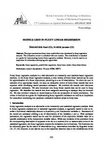
The model with objective function (2.8) and restrictions (2.3)-(2.5) will be called Quadratic Possibilistic Model (QPM) in this paper, and with the parameters QP M (k1 , k2 ). The following proposition guarantees that this last model does not depend on the data unit. One of the main criticisms to possibilistic regression analysis is that the number of available data increases, the length of estimated spreads also increases. In this context, we propose a new model, called Quadratic Non-Possibilistic (QNP), which considers the objective function (2.8) and which incorporates the only restriction (2.5). Example: these data are taken from [14] where X goes from 1 to 8. First, we have applied the model of Kim[7] and Chang[2] with X varying from 1 to 22. The results of this analysis are depicted in Fig. 1. As can be

5


observed, when X=15, the three curves converge (ai = ai − cLi = ai + cRi ). With values higher than 15 the relationship among extreme points in the estimated membership functions reverses, so that the left extreme is higher than the right extreme (which is an inconsistent result). 700

Estimated fuzzy valuies

600 500 400

p

300

c q

200 100

484

441

400

361

324

289

256

225

196

81

169

64

144

49

121

36

100

25

2

9

4

1

16

1

0 3

4

5

6

7

8

9 10 11 12 13 14 15 16 17 18 19 20 21 22

variable X

Figure 1: Predictions with methods of Kim [7] and Chang [2]

600

400

p c

300

q 200 100

144 169 196 225 256 289 324 361 400 441 484

0 1 4 9 16 25 36 49 64 81 100 121

Estimated fuzzy valuies

500

1 2 3 4 5 6 7 8 9 10 11 12 13 14 15 16 17 18 19 20 21 22 variable X

Figure 2: Predictions with method QNP

6


The same experimentation with Model QNP is depicted in Figure 2. Model QNP forces the estimate’s structure to be the same for both the central tendency and the fuzzy extremes. This fact, which can be seen as a restriction in the behavior of the spreads, guarantees that the inconsistencies of the previous example do not appear. This predictive capability of the proposed model overcomes the limitation analyzed by Kim et. al [7], where the capability of prediction is restricted only to probabilistic models.

3

Fuzzy Ridge regression

The approach based on quadratic programming analyzed in previous sections has the additional advantage of allowing the management of multicollinearity. With this approach, we can set regression methods which deal with the problem of multicollinearity among input variables, as for example, fuzzy ridge regression. In the seminal paper of fuzzy regression, Tanaka et al. [15] stated about their concrete example “the fact that A4 and A5 are negative depends on the strong correlations between variables X4 and X5 ”. Actually, the correlation between X1 and X5 is 0.95, much higher than any other value of correlation in Y and Xi , which indicates a very high multicollinearity. It can be assumed that the same distortion effect that affects probabilistic regression can be found in fuzzy regression. The most popular probabilistic regression techniques used to face multicollinearity are the regression of principal components and the Ridge regression. Recently, papers about fuzzy Ridge regression has appeared in the literature which use an approach closely related to the support vector machine proposed by Vapnik[4, 5]. In the area of probabilistic regression, Ridge regression can be seen as a correction of the matrix X‘X. This matrix, in presence of multicollinearity, has values close to zero. It can be proven that the expected value for estimations a 0 a is E(ae0 e a) = a a + σ 2 0

X ³ cte ´ i

λi

(3.1)

7


where λi are the eigenvalues values of X’X and ”cte” is a constant. If these values are close to 0, the expected value for a 0 a increases a lot, producing coefficients with high absolute value and with the opposite sign, as the comment of Tanaka et al. suggests. The introduction of a small positive value in the diagonal of X’X moves the least value of λi far from zero, and, thus, the expected value for a 0 a decreases. The Ridge regression can be seen as the addition of a new factor to the objective function. This factor depends on a parameter λ, called Rigde parameter. Ridge regression minimizes the conventional criterion of least squares in the following way [3]: aridge = min a

hX i

(yi −

X

Xij ai )2 + λ

j

X

a2j

i (3.2)

j

The Ridge solutions are not equivariant under changes in the scale of the inputs. The model of Fuzzy Ridge regression (FRR) is introduced with the following objective function: P P 0 0 0 k1 ni=1 (yi − a Xi )2 + k2 ( ni=1 (yi − pi − (a − cL )Xi )2 + +

n m X X 0 0 (yi + qi − (a + cR )Xi )2 ) + λ( (a2j + c2Lj + c2Rj )) i=1

(3.3)

j=1

There exist many proposals to chose λ. Many of them suggest varying the parameter in a certain interval, checking the behavior of the coefficients, and chosing λ when the estimates stay stable. A more general approach can be proposed, where the λ Ridge parameter depends on each variable (λi with i = 1, .., m). In this case, the objective function is as follows P P 0 0 0 k1 ni=1 (yi − a Xi )2 + k2 ( ni=1 (yi − pi − (a − cL )Xi )2 +

+

m n X X 0 0 λi (a2i + c2Li + c2Ri )) (yi + qi − (a + cR )Xi )2 ) + ( i=1

i=1

(3.4)

8 3.1


An example

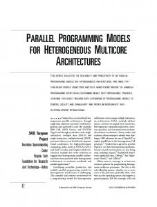
The example, similar to the one used for Tanaka [15]to illustrate the problem of multicollinearity, will be used here to experiment with the previously defined Fuzzy Ridge regression model. We will use the method QPM, with k1 = 1 and k2 = 1 for our calculus. Figure 3 depicts the trajectory of the coefficients’ centers, when the λi parameters are function of the diagonal of the matrix X’X (from 0 to 1 with increments of 0.1).

2500

Estimated central coefficients

2000 1500

a1

1000

a2

500

a3

0

a4

-500

a5 a6

-1000 -1500 -2000

0

0,1

0,2

0,3

0,4

0,5

0,6

0,7

0,8

0,9

1

Ridge parameter

Figure 3: Central coefficients, ai , as λi increases

According to the example of Tanaka et al. (Y is the price of a house), all the coefficients must be positive (maybe with the exception of the number of Japanese rooms) because as the value of the variable increases the value of the house must also increase. The regression analysis, either of least squares or our fuzzy regression, initially produces some negative coefficients. However, three coefficients, which initially have negative values, reach positive values. If we suppose that the λ coefficients are constant, varying from 0 to 55, we have the trajectory for the coefficients’ centers depicted in figure 4. As can be observed, one of the coefficient remains negative while the other two

9


become positive.

2500


2000

a1

1500

a2 1000

a3 a4

500

a5 0

a6

-500

-1000

0

5

10

15

20

25

30

35

40

45

50

Ridge parameter

Figure 4: Ridge central coefficients, ai , as λ increases

In any case, the availability of more reliable coefficients permits a better knowledge of the function we are looking for, and, consequently, better conditions for the use with predictive aims. In order to end this section, let us compare our model with the model of Hong and Hwang[4, 5]. These authors do a dual estimation of the coefficients, with the relation: βdual = Y 0 (XX 0 + Iλ)−1 X

(3.5)

where I is the identity matrix of range n and λ is a constant, the Ridge coefficient, whose values increase in value from 0. If we take the same data, and make λ increase from 0 to 1.5 (with increments of 0.1) we obtain the results depicted in figure 5. These results must be contrasted with those of figure 4, where the ridge parameter is also constant. As can be observed, central coefficients have a similar behavior in both graphics: there is a positive coefficient which converges to (approximately) 1300 and a negative coefficient which converges

10



3400

2400

a1 a2

1400

a3 a4 a5

400

a6 -600

-1600 0

0.1 0.2

0.3

0.4

0.5

0.6

0.7

0.8

0.9

1

1.1

1.2

1.3

1.4

1.5

ridge parameter

Figure 5: Dual ridge central coefficients of Hong and Hwang, Betadual as λ increases

to (approximately) -600. The other coefficients are close to zero. However, the main difference is in the central coefficient a1 . With the method of Hong and Hwang, this coefficient has a high value when λ = 0 and is -600 when λ = 0.1. This fact does not occurs with our method.

4

Conclusions

In this paper we have tried to validate the use of quadratic programming (quadratic objective functions) in order to obtain a good fitness in fuzzy linear regression. To accomplish this task, we have adapted one existing model (ETM) and have proposed two new models (QPM and QNP). Method QPM is a good choice when possibilistic restrictions are important in the problem. If we do not want to pay special attention to the possibilistic restriccions, QNP is an appropriate alternative. We have proposed a special version of Fuzzy Ridge Regression based


11

on our previous study on quadratic methods in order to cope with the multicollinearity problem.

References [1] A. B´ardossy. Note on fuzzy regression. Fuzzy Sets and Systems, 37:65– 75, 1990. [2] Yun-His O. Chang. Hybrid fuzzy lest-squares regression analysis and its reliability measures. Fuzzy Sets and Systems, 119:225–246, 2001. [3] T. Hastre, R. Tibshirani, and J. Friedman. The element of Statistical Learning. Data Mining, Inference, and Prediction. 2001. [4] D. H. Hong and C. Hwang. Ridge regression procedure for fuzzy models using triangular fuzzy numbers. Fuzziness and Knowledge-Based Systems, 12:2:145–159, 2004. [5] D. H. Hong, C. Hwang, and C. Ahn. Ridge estimation for regression models with crisp input and gaussian fuzzy output. Fuzzy Sets and Systems, 142:2:307–319, 2004. [6] C. Kao and C.L. Chyu. Least-squares estimates in fuzzy regression analysis. European Journal of Operational Research, 148:426–435, 2003. [7] B. Kim and R.R. Bishu. Evaluation of fuzzy linear regression models by comparing membership functions. Fuzzy Sets and Systems, 100:342– 353, 1998. [8] K. J. Kim, H. Moskowitz, and M. Koksalan. Fuzzy versus statistical linear regression. European Journal of operational Research, 92:417– 434, 1996. [9] E. C. Ozelkan and L. Duckstein. Multi-objective fuzzy regression: a general framework. Computers and Operations Research, 27:635–652, 2000. [10] G. Peters. Fuzzy linear regression with fuzzy intervals. Fuzzy Sets and Systems, 63:45–53, 1994.

12


[11] D. T. Redden and W. H. Woodall. Properties of certain fuzzy linear regression methods. Fuzzy Sets and Systems, 64:361–375, 1994. [12] K. Sugihara, H. Ishii, and H. Tanaka. Conjoint analysis based on rough approximation by dominance relations using interval. International Journal of Aproximate Reasoning, 1:221–242, 1987. [13] H. Tanaka and J. Wataka. Possibilistic linear systems and their applications to the linear regresion model. Fuzzy Sets and Systems, 27:275– 289, 1988. [14] Hideo Tanaka and Haekwan Lee. Interval regression analysis by quadratic programming approach. IEEE Trans. on Fuzzy Systems, 6(4), 1998. [15] Hideo Tanaka, S. Uejima, and K. Asai. Linear regression analysis with fuzzy model. IEEE Trans. on Systems, Man, and Cybernetics, 12(6):903–907, 1982. [16] F-M. Tseng and L. Lin. A quadratic interval logit model for forescasting bankruptcy. omega. The International Journal of Management Science, In press. [17] L. A. Zadeh. The concept of a linguistic variable and its application to aprox´ımate reasoning i, ii, iii. Information Sciences, 8-9:199–251, 301–357, 43–80, 1999.