to perform machine learning tasks such as classification and clustering. ... the construction method we propose builds fuzzy prototypes: the fuzzy logic framework ...
M.-J. Lesot, M. Rifqi et B. Bouchon-Meunier. Fuzzy prototypes: From a cognitive view to a machine learning principle. In H. Bustince, F. Herrera and J. Montero editors, Fuzzy Sets and Their Extensions: Representation, Aggregation and Models, (pp. 431-452). Springer. 2007.
Fuzzy prototypes: From a cognitive view to a machine learning principle Marie-Jeanne Lesot1 , Maria Rifqi1 , and Bernadette Bouchon-Meunier1 Universit´e Pierre et Marie Curie-Paris6, CNRS, UMR 7606, LIP6, 8, rue du Capitaine Scott, Paris, F-75015, France {marie-jeanne.lesot,maria.rifqi,bernadette.bouchon-meunier}@lip6.fr Abstract. Cognitive psychology works have shown that the cognitive representation of categories is based on a typicality notion: all objects of a category do not have the same representativeness, some are more characteristic or more typical than others, and better exemplify their category. Categories are then defined in terms of prototypes, i.e. in terms of their most typical elements. Furthermore, these works showed that an object is all the more typical of its category as it shares many features with the other members of the category and few features with the members of other categories. In this paper, we propose to profit from these principles in a machine learning framework: a formalization of the previous cognitive notions is presented, leading to a prototype building method that makes it possible to characterize data sets taking into account both common and discriminative features. Algorithms exploiting these prototypes to perform tasks such as classification or clustering are then presented. The formalization is based on the computation of typicality degrees that measure the representativeness of each data point. These typicality degrees are then exploited to define fuzzy prototypes: in adequacy with human-like description of categories, we consider a prototype as an intrinsically imprecise notion. The fuzzy logic framework makes it possible to model sets with unsharp boundaries or vague and approximate concepts, and appears most appropriate to model prototypes. We then exploit the computed typicality degrees and the built fuzzy prototypes to perform machine learning tasks such as classification and clustering. We present several algorithms, justifying in each case the chosen parameters. We illustrate the results obtained on several data sets corresponding both to crisp and fuzzy data.
1 Introduction Prototypes are elements representing categories, structuring and summarizing them, underlining their most important characteristics and their specificity as opposed to other categories. From a cognitive point of view, they are the basis for the categorization task, process that aims at considering as equivalent objects that are distinct but similar: cognitive science works [31,32] showed
2
Marie-Jeanne Lesot, Maria Rifqi, and Bernadette Bouchon-Meunier
that natural categories are organized around the notion of prototype and the related notion of typicality. In this paper, we propose to transpose the cognitive view of prototypes to a machine learning principle to extract knowledge from data. More precisely, we propose to characterize data sets through the construction of prototypes that realize the cognitive approach. The core of our motivation is the fact that, through this notion of prototype, a data subset (a category for instance) is characterized both from an internal and an external point of view: the prototype underlines both what is common to the subset members and what is specific to them in opposition to the other data. Using these two complementary components leads to context-dependent representatives that are more relevant than classic representatives that actually exploit only the internal view. Furthermore, the method makes it possible to determine the extent to which the prototype should be a central or a discriminative element, i.e. it allows to rule the relative importance of common and discriminative features, leading to a flexible prototype building method. Another concern of our approach is the adequacy with human-like descriptions that are usually based on imprecise linguistic expressions. To that aim, the construction method we propose builds fuzzy prototypes: the fuzzy logic framework makes it possible to model sets with unsharp boundaries or vague and approximate concepts, as occur in this framework. The paper is organized as follows: in Section 2, the cognitive definitions of typicality and prototypes are introduced. In Section 3, these principles are formalized to a prototype building method that makes it possible to characterize numerical data sets. These prototypes are then exploited both for supervised and unsupervised learning: Section 4 presents prototype-based classification methods and Section 5 describes a typicality-based clustering algorithm.
2 Cognitive definition of prototype The cognitive definition of prototype was first proposed in the 70’s [27] and popularized by E. Rosch [31,32], in the context of the study of cognitive concept organization. Previously, a crisp relationship between objects and categories was assumed, based on the existence of necessary and sufficient properties to determine membership: according to this model, an object belongs to a category if it possesses the properties, interpreted as necessary and sufficient conditions; otherwise, it is not a member of the category. Now in the case of natural categories, it is often the case that no feature is common to all the category members: as modeled in the family resemblance model of Wittgenstein [36], each object shares different common features with other members of the category, but no globally shared feature can be identified. The prototype view of concept organization [27,31,32] models categories as organized around a center, the prototype, that is described by means of properties that are characteristic, typical of the category members. Indeed, all
Fuzzy prototypes: From a cognitive view to a machine learning principle
3
objects in a category are not equivalent: some are better examples and more characteristic of the category than others. For instance, in the case of the mammal category, the dog is considered as a better example than a platypus. Thus, objects are spread over a scale, or a gradient of typicality; the prototype is then related to the individuals that maximize this gradient. Rosch and her colleagues [31,32] studied this typicality notion and showed it depends on two complementary components: an object is all the more typical of its category as it shares many features with the other members of the category and few features with the members of other categories. This can for instance be illustrated by platypuses and whales in the case of mammals: platypuses are atypical mainly because they have too few features in common with other mammals, whereas whales are atypical mainly because they have too many common features with members of the fish category. Due to this typicality definition, prototypes underline both the common features of the category members and their discriminative features as opposed to other categories: they characterize the category both internally and in opposition to other categories.
3 Realization of the prototype view 3.1 Principle To construct a fuzzy prototype in agreement with the previous cognitive prototype view, we consider that the degree of typicality of an object depends positively on its total resemblance to others objects of its class (internal resemblance) and on its total dissimilarity to objects of other classes (external dissimilarity). This makes it possible to consider both the common features of the category members, and their distinctive features as opposed to other categories. More precisely, the fuzzy prototype construction principle consists in three steps [29]: Step 1 Compute the internal resemblance degree of an object with the other members of its category and its external dissimilarity degree with the members of the outside categories. Step 2 Aggregate the internal resemblance and the external dissimilarity degrees to obtain the typicality degree of the considered object. Step 3 Aggregate the objects that are typical ”enough”, i.e. with a typicality degree higher than a predefined threshold to obtain the fuzzy prototype. Internal resemblance and external dissimilarity Step 1, that is illustrated on figure 1, requires the choice of a resemblance measure and a dissimilarity measure to compare the objects. These measures depend on the data nature and are detailed in Sections 3.3 and 3.4 in the case
4
Marie-Jeanne Lesot, Maria Rifqi, and Bernadette Bouchon-Meunier
(a)
(b)
Fig. 1. (a) Computation of the internal resemblance, as the resemblance to the other members of the category, (b) computation of the external dissimilarity, as the dissimilarity to members of the other categories.
of fuzzy and crisp data. Formally, denoting them r and d respectively, and denoting x an object belonging to a category C, x internal resemblance with respect to C, R(x, C), and its external dissimilarity, D(x, C), are computed as R(x, C) = avg(r(x, y), y ∈ C) D(x, C) = avg(d(x, y), y 6∈ C) (1) i.e. as the average resemblance to other members of the category and the average dissimilarity to members of other categories. The average operator can be replaced with other operators [29]. Figure 2 illustrates these definitions in the case of the iris data base, using only one attribute (petal length) for visualization sake: the histograms represent the data distribution, ∗, + and ◦ respectively depict the three classes; the y-axis shows for each point its internal resemblance and external dissimilarity. As expected, it can be seen that the points maximizing internal resemblance are, for each class, the central points, underlining the common features of the category members. On the contrary, the points maximizing the external dissimilarity are extreme points, at least for the two extreme classes: points in the middle class (+ class) get low external dissimilarity values, as they are too close to the other groups and correspond to an average behavior. Thus external dissimilarity underlines the specificity of the classes, for instance indicating that high petal length is characteristic for the ◦ class: it highlights the discriminative features of each category (or the absence of any, for the + class), and makes it possible to build caricatures of the classes. Therefore combining both information to a typicality degree makes it possible to build representatives that simultaneously underline the common features of the category members, as well as their discriminative features as opposed to other categories.
Fuzzy prototypes: From a cognitive view to a machine learning principle 1
1
0.9
0.9
0.8
0.8
0.7
0.7
0.6
0.6
0.5
0.5
0.4
0.4
0.3
0.3
0.2
0.2
0.1
0
5
0.1
1
2
3
4
5
6
7
0
(a)
1
2
3
4
5
6
7
(b)
Fig. 2. (a) Internal resemblance, (b) external dissimilarity, for the iris data set, considering only the petal length attribute [23].
Aggregation to a typicality degree Step 2 requires the choice of an aggregation operator to express the dependence of typicality on internal resemblance and external dissimilarity, that is formally written T (x, C) = ϕ(R(x, C), D(x, C)) (2) where ϕ denotes the aggregation operator. It makes it possible to rule the semantics of typicality and thus that of the prototypes, determining the extent to which the prototype should be a central or a discriminative element [23]. Figure 3 illustrates the typicality degrees obtained from the internal resemblance and external dissimilarity of figure 2 for four operators: the minimum (see fig. 3a) is a conjunctive operator that requires both R and D to be high for a point to be typical, leading to rather small typicality degrees on average. On the contrary, for the maximum (see fig. 3b), as any disjunctive operator, if either R or D is high, a point is considered as typical. This leads to higher values but to non-convex distributions, reflecting a double semantics for typicality: central points as well as extreme points are typical, but for different reasons. Trade-off operators, such as the weighted mean (fig. 3c), offer a compensation property: low R values can be compensated for by high D. This is illustrated by the leftmost point on fig. 3c, whose typicality is higher than with the min operator, because its external dissimilarity compensates for its internal resemblance. The weights used in the weighted mean determine the extent to which compensation can take place, and rule the relative importance of internal resemblance and external dissimilarity, leading to more or less discriminative prototypes, underlying more the common or the distinctive features of the categories. Lastly, variable behavior operators, such as the mica operator [17] (see fig. 3d) or the symmetric sum [33], are conjunctive, disjunctive or trade-off operators, depending on the values to be aggregated. They offer a reinforcement property: if both R and D are high, they reinforce each other to give an
6
Marie-Jeanne Lesot, Maria Rifqi, and Bernadette Bouchon-Meunier 1
1
0.9
0.9
0.8
0.8
0.7
0.7
0.6
0.6
0.5
0.5
0.4
0.4
0.3
0.3
0.2
0.2
0.1
0
0.1
1
2
3
4
5
6
7
0
1
2
3
(a) 1
1
0.9
0.9
0.8
0.8
0.7
0.7
0.6
0.6
0.5
0.5
0.4
0.4
0.3
0.3
0.2
0.2
0.1
0
4
5
6
7
5
6
7
(b)
0.1
1
2
3
4
5
(c)
6
7
0
1
2
3
4
(d)
Fig. 3. Typicality degrees obtained from the internal resemblance and the external dissimilarity shown on fig. 2 using different aggregation operators: (a) T = min(R, D), (b) T = max(R, D), (c) T = 0.6R + 0.4D, (d) T =mica(R,D) [17].
even higher typicality (see class ∗), if both are low, they penalize each other to give an even smaller value (see the leftmost point of the ◦ class). Therefore, the aggregation operator determines the semantics of typicality, and rules the relative influence played by internal resemblance and external dissimilarity. Aggregation to a prototype Lastly step 3 builds the prototype of a category itself, as the aggregation of the most typical objects of the category: the prototype for category C is defined in a general form as p(C) = ψ({x/T (x, C) > τ }) (3) where τ is the typicality threshold and ψ the aggregation operator. The latter can still depend on the typicality degrees associated to the selected points, taking for instance the form of a weighted mean. Its actual definition depends on the data nature, it is detailed in Sections 3.3 and 3.4 in the case of fuzzy and crisp data. Remarks It is to be underlined that prototype can be built either from the typicality degrees of objects, as presented above, but also in an attribute per attribute
Fuzzy prototypes: From a cognitive view to a machine learning principle
7
approach: the global approach makes it possible to take into account attribute correlation, but it can also be interesting to enhance the typical values of the different properties used to describe the objects, without considering an object as an indivisible whole. This means, all the values of a property are considered simultaneously, without taking into account the objects they describe. For instance, if the objects are represented by means of a color, a size and a weight, the fuzzy prototype of the category of these objects is the union of typical values for the color, the size and the weight. It means that instead of computing internal resemblance, external dissimilarity and typicality degrees for each object, these quantities are computed for each attribute value. This approach is in particular applied in the case of fuzzy data, as described in Section 3.3. 3.2 Related works There exist many works to summarize data sets, or build significant representatives. A first approach, taking the average as starting point, consists in defining more sophisticated variants to overcome the average’s drawbacks, in particular its sensitivity to outliers (see for instance [11]). Among these variants, one can mention the Most Typical Value [11] or the representatives proposed in [26] or [37]. In all these cases, the obtained value is computed as a weighted mean, the difference comes from the ways the weights are defined. Besides, a second approach, more concerned with interpretability, does not reduce the representative to a single precise value but builds so-called linguistic summaries [16,15]. The latter identify significant trends in the data and represent them in the form “Q B’s are A” where Q is a linguistic quantifier and A and B are fuzzy sets; for example, “most important experts are young”. Yet, both approaches build internal representatives that take into account the common characteristics of the data, but not their specificity. More precisely, they focus only on the data to be summarized, and do not depend on their context, which prevents them from identifying their particularity. On the contrary, the cognitive view highlights the discriminative features: the data are also characterized in opposition to the other categories. Furthermore, the proposed realization of the cognitive approach described in Section 3.1 makes it possible to rule the relative importance common and discriminative features play and the trade-off between them through the choice of the aggregation operator, leading to a flexible method. As illustrated in Section 4 and 5, the choice of the aggregation operator depends on the considered use of the prototype. 3.3 Fuzzy data case In this section, we consider the case of fuzzy data, i.e. data whose attributes take as values fuzzy sets: formally, denoting F (R) the set of fuzzy subsets defined on the real line, the input space is F (R)p where p denotes the number of
8
Marie-Jeanne Lesot, Maria Rifqi, and Bernadette Bouchon-Meunier
attributes. We describe the instantiation of the previous prototype construction method, discussing comparison measures for such data and aggregation operators to construct the prototypes from the most typical values. We then present an application in a medical domain, to mammographies. Comparison measures In the case of fuzzy data, the framework used to compute the internal resemblance as well as the external dissimilarity is the one defined in [4] generalizing the Tversky’s ”contrast model” [35]. In this framework a measure of resemblance comparing two fuzzy sets A and B is a function of three arguments: M (A ∩ B) (the common features), M (A − B) and M (B − A) (the distinctive features), where M is fuzzy set measure [9] like the fuzzy cardinality for instance. More formally [4]: Definition 1 A measure of resemblance r is – non decreasing in M (A ∩ B), non increasing in M (A − B) and M (B − A) – reflexive: ∀A, r(A, A) = 1 – symmetrical: ∀A, B, r(A, B) = r(B, A) An example of measure of resemblance, proposed by [8], generalizing the Jacccard measure to fuzzy sets, is the following: r(A, B) = M (A ∩ B)/M (A ∪ B) forM such that : M (A ∪ B) = M (A ∩ B) + M (A − B) + M (B − A). We also refer to this framework to choose a dissmilarity measure: Definition 2 A measure of dissimilarity d is: – independent of M (A ∩ B) and non decreasing in M (A − B) and M (B − A) – minimal: ∀A, d(A, A) = 0 An example of measure of dissimilarity, based on the generalized Minkowski’s distance, is the following: d(A, B) =
�
1 Z
�Z
��1/n |fA (x) − fB (x)|n dx
where Z is a normalizing factor, n an integer and fX denotes the membership function of the fuzzy set X. It is to be noticed that a dissimilarity measure is not necessarily deduced from a resemblance measure and vice versa because the purpose is to have different information when comparing two objects, the dissimilarity measure focusing on distinctive features.
Fuzzy prototypes: From a cognitive view to a machine learning principle
9
Aggregation into a fuzzy prototype In the last step of the fuzzy prototype construction, fuzzy values of an attribute that are typical ”enough” have to be aggregated in order to obtain a typical value for the considered attribute. An aggregation operator must be chosen among numerous existing operators, deeply studied by several authors like Mizumoto [24], [25], Detyniecki [7] or Calvo and her colleagues [5]. Application to mammography Nowadays, mammography is the primary diagnostic procedure for the early detection of breast cancer. Microcalcification1 clusters are an important element in the detection of breast cancer. This kind of finding is the direct expression of pathologies which may be benign or malignant. The description of microcalcifications is not an easy task, even for an expert. If some of them are easy to detect and to identify, some others are more ambiguous. The texture of the image, the small size of objects to be detected (less than one millimeter), the various aspects they have, the radiological noise, are parameters which impact the detection and the characterization tasks. More generally, mammographic images present two kinds of ambiguity: imprecision and uncertainty. The imprecision on the contour of an object comes from the fuzzy aspect of the borders: the expert can define approximately the contour but certainly not with a high spatial precision. The uncertainty comes from the microcalcification superimpositions: because objects are built from the superimpositions of several 3D structures on a single image, we may have a doubt about the contour position. The first step consists in finding automatically the contours of microcalcifications. This segmentation is also realized thanks to a fuzzy representation of imprecision and uncertainty (more details can be found in [28]). Each microcalcification is then described by means of 5 fuzzy attributes computed from its fuzzy contour. These attributes enable us to describe more precisely: • •
the shape (3 attributes): elongation (minimal diameter/maximal diameter), compactness1, compactness2. the dimension (2 attributes): surface, perimeter.
Figure 4 shows an example of the membership functions of the values taken by a detected microcalcification. One can notice that the membership functions are not ”standard” in the sense that they are not triangular or trapezoidal (as it is often the case in the literature) and this is because of the automatic generation of fuzzy values (we will not go into details here, interested readers may refer to [3]). Experts have categorized microcalcifications into 2 classes: round microcalcifications and not round ones, because this property is important to qualify 1
The microcalcifications are small depositions of radiologically very opaque materials which can be seen on mammography exams as small bright spots.
10
Marie-Jeanne Lesot, Maria Rifqi, and Bernadette Bouchon-Meunier 1.2
1.2 1 Membership degree
Membership degree
1 0.8 0.6 0.4 0.2
0.6 0.4 0.2
0
0 0
10
20
30
40 50 Surface
60
70
80
140 160 180 200 220 240 260 280 300 Elongation
1.2
1.2
1
1 Membership degree
Membership degree
0.8
0.8 0.6 0.4 0.2
0.8 0.6 0.4 0.2
0
0 100
120
140 160 180 200 Compactness1
220
10
20 30 Perimeter
40
240
0
2
4
6 8 10 Compactness2
12
14
1.2
Membership degree
1 0.8 0.6 0.4 0.2 0 0
50
Fig. 4. Description of a microcalcification by means of fuzzy values of its 5 attributes.
the malignancy of the microcalcifications. The aim is then to build the fuzzy prototypes of the classes round and not round. Figure 5 gives the obtained fuzzy prototypes with the internal resemblance and external dissimilarity computed using as aggregator the median (replacing the average in equation (1) by the median). The typicality degrees are obtained by the probabilistic tconorm (ϕ(x, y) = x + y − x · y in equation (2)). Lastly, the fuzzy values with maximal typicality degree are aggregated through the max-union operator to define the fuzzy prototype value of the corresponding attribute. It can be seen that on the attributes elongation, compactness1 or compactness2, the typical values of the two classes round and not round, are quite different: the intersection between them is low. This can be interpreted in the following way: a round microcalcification typically has an elongation approximately between 100 and 150 whereas a not round microcalcification typically has an elongation approximately between 150 and 200, etc. For the attributes surface and perimeter, contrary to the previous attributes, the typical values
Fuzzy prototypes: From a cognitive view to a machine learning principle ROUND
NOT ROUND
1.2
1.2 1 Membership degree
Membership degree
1 0.8 0.6 0.4 0.2
20 30 Surface
40
50
0
1.2
1.2
1
1 Membership degree
Membership degree
10
0.8 0.6 0.4 0.2
10
20 30 Surface
40
50
0.8 0.6 0.4 0.2
0
0 100
150
200 Elongation
250
300
100
1.2
150
200 Elongation
250
300
1.2 1 Membership degree
1 Membership degree
0.4
0 0
0.8 0.6 0.4 0.2
0.8 0.6 0.4 0.2
0
0 50
100 150 Compactness1
200
250
50
1.2
100 150 Compactness1
200
250
15
20
1.2 1 Membership degree
1 Membership degree
0.6
0.2
0
0.8 0.6 0.4 0.2
0.8 0.6 0.4 0.2
0
0 0
5
10 Compactness2
15
20
0
1.2
5
10 Compactness2
1.2 1 Membership degree
1 Membership degree
0.8
0.8 0.6 0.4 0.2
0.8 0.6 0.4 0.2
0
0 0
5
10
15 20 Perimeter
25
30
0
5
10
15 20 Perimeter
25
Fig. 5. Prototypes of the classes round and not round.
30
11
12
Marie-Jeanne Lesot, Maria Rifqi, and Bernadette Bouchon-Meunier
of the two classes are superimposed, it means that these attributes are not typical. 3.4 Crisp data case In this section, we consider the case of crisp numerical data, i.e. data represented as real vectors: the input space is Rp , where p denotes the number of attributes. We describe the comparison measures that can be considered in this case, and the aggregation operator that builds prototypes from the most typical data; lastly we illustrate the results obtained on a real data set. Comparison measures Contrary to the previous fuzzy data, for crisp data, the relative position of two data cannot be characterized by their common and distinct elements respectively represented as their intersection and their set differences: the information is reduced, and depends on a single quantity, expressed as a distance or a scalar product of the two vectors. Thus dissimilarity is simply defined as a normalized distance [19] � � � � δ(x, y) − dm ,1 ,0 (4) d(x, y) = max min dM − dm where δ is a distance, for instance chosen among the Euclidean, the weighted Euclidean, the Mahalanobis or the Manhattan distances, depending on the desired properties (e.g. robustness, derivability). The parameters dm and dM are the normalization parameters, that can for instance be chosen as dm = 0 and dM the maximum observed distance. More generally, dm can be interpreted as a tolerance threshold, indicating the distance below which the dissimilarity is considered as 0, i.e. no distinction is made between the two data points; dM corresponds to a saturation threshold, indicating the distance from which the two points are considered as totally dissimilar. Regarding resemblance measures, two definitions can be considered. They can first be deduced from scalar products as the latter are related to the angle between the two vectors to be compared and are maximal when the two vectors are identical; they must be normalized too to define a resemblance measure. Besides, similarity can be defined as a decreasing function of dissimilarity, as for instance r(x, y) = 1 − d(x, y)
or
r(x, y) =
1 1 + d(x, y)γ
(5)
where γ is a user-defined parameter. Indeed, if dissimilarity is total, resemblance is 0 and reciprocally. The Cauchy function on the right expresses a nonlinear dependency between resemblance and dissimilarity, and in particular makes it possible to rule the discrimination power of the measure [30,19].
Fuzzy prototypes: From a cognitive view to a machine learning principle
13
It is to be noticed that, as in the case of fuzzy data, the resemblance measure is not necessarily the complement to 1 of the dissimilarity measure: the normalization parameters defining dissimilarity can be different from those used to define the dissimilarity from which the resemblance is deduced. Indeed, resemblance is used to compare data points belonging to the same category, whereas dissimilarity compares points from different categories. Thus it is expected that they apply to different distance scales, requiring different normalization schemes. Aggregation into a fuzzy prototype After the typicality degrees have been computed, the prototype is defined as the aggregation of the most typical data. In the case of numerical data, one can for instance define the prototype as the weighted average of the data, using the typicality degrees as weights. Yet this reduces the prototype to a single precise value, which is not in adequacy with human-like description of categories: considering for instance data describing the height of persons from different countries, one would rather say that ”the typical French person is around 1.70m tall” instead of ”the typical French person is 1.6834m tall” (fictitious value): the prototype is not described with a single numerical value, but with a linguistic expression, ”around 1.70m”, which is imprecise. This is better modeled in the fuzzy set framework, that makes it possible to represent such unclear boundaries. Therefore we propose to aggregate the most typical data in a fuzzy set [23]. To that aim, two thresholds are defined, respectively indicating the minimum typicality degree required to belong to the prototype kernel and its support; in-between, a linear interpolation is performed. In our experiments, the thresholds are set to high values (respectively 0.9 and 0.7), because the prototype aim is to characterize the data set, and extract its most representative components, and not to describe it as a whole. Application to student characterization As an example, we consider a data set describing results obtained by 150 students to two exams [23]. It was decomposed into 5 categories by the fuzzy cmeans [10,2]: the central group corresponds to students having average results for both exams, the 4 peripheral clusters correspond to the 4 combinations success/failure for the two exams. Prototypes are built to characterize these 5 categories. The comparison measures are based on normalized Euclidean distances (with different normalization factors for the dissimilarity and the resemblance). The typicality degrees are derived from internal resemblance and external dissimilarity using the symmetric sum operator [33]. Lastly the prototype is derived from the most typical data points using the method described in the previous paragraph.
14
Marie-Jeanne Lesot, Maria Rifqi, and Bernadette Bouchon-Meunier 1
20 0.9
18 16
0.8
14
0.7
12
0.6
10 0.5
8 6
0.4
4
0.3
2
0.2
0 0
5
10
15
20
0.1
Fig. 6. Level lines of the 5 fuzzy prototypes characterizing students described by their results on two exams [23].
Figure 6 represents the level lines of the obtained prototypes and shows they provide much richer information than a single numerical value: they model the unclear boundaries of the prototypes. They also underline the difference between the central group and the peripheral ones: no point totally belongs to the prototype of the central group, because it has no real specificity as opposed to the other categories, as it corresponds to an average behavior. In all cases, the fuzzy prototypes characterize the subgroups, capturing their semantics: they are approximately centered around the group means but take into account the discriminative features of the clusters and underline their specificity. For instance, for the lower left cluster, the student having twice the mark 0 totally belongs to the prototype, which corresponds to the group interpretation as students having failed at both exams and underline its specificity. It is to be noticed that this results from the chosen aggregation operator (symmetric sum [33]) that gives a high influence for external dissimilarity: it can be the case that such an extreme case should have a lower membership degree, which can be obtained changing the aggregation operator.
4 Extension to supervised learning: classification In this section, we exploit the previous formalization of the typicality degrees as well as the fuzzy prototype notion to perform a supervised learning task of classification. It is true that the major interest of a prototype comes from its power of description thanks to its synthetic view of the database. But, as Zadeh underlined [38], a fuzzy prototype can be seen as a schema for generating a set of objects. Thus, in a classification task, when a new object has to be classified, it can be compared to each fuzzy prototype and classified in the
Fuzzy prototypes: From a cognitive view to a machine learning principle
15
Table 1. Classification results for the 3 typicality-based methods and for the instance-based learning algorithm (IBL) (in percentage of good classification). round/not round elongated/not elongated mall/not small
Method 1 Method 2 Method 3 75.00 79.63 82.41 79.41 80.88 79.41 92.45 93.71 91.82
IBL 79.63 73.53 91.82
class of the nearest prototype (a sort of nearest neighbor algorithm where the considered neighbors are only the prototypes of the classes). Another approach consists in taking into account the degrees of typicality without considering the fuzzy prototypes, it means that the last step of our construction processed is missed. The difference of our approach with an instance-based learning algorithm [1] is that our methods are not lazy: the information learned during the typicality degree computation is taken into account in the classification task, more precisely in the class setting step, either by considering the nearest prototypes or by weighting the comparison by the typicality degrees. We proposed three classification methods based on typicality or on prototype notions: •
•
•
The first one is the one described above giving the class of the nearest prototype of the object to be classified. The prototype is constructed with the fuzzy value maximizing the typicality degree. The second one is like the first one, but the fuzzy prototype is obtained aggregating by the union (the maximum) of the values with a high typicality degree whereas the first one considers only one value. In the third one, a new object is compared to each object of the learning database. The comparison is the aggregation of the attribute by attribute comparisons weighted by the degree of typicality of the attribute value of the object in the learning database. Then, the class given to the unknown object is the class of the most similar object in the learning database. It is also possible to consider the k most similar objects but the realized experiments consider only the closest object relatively to the weighted similarity.
We tested these 3 methods on the microcalcifications database presented in Section 3.3 in 3 different classification problems: to classify the microcalcifications in round/not round, elongated/not elongated and small/not small. Table 1 gives the highest good classification rates obtained by each method and compares them with instance-based algorithm (IBL) with 10 neighbors. It shows that our method classifies better than IBL, highlighting the gain provided by the typicality-based approaches.
16
Marie-Jeanne Lesot, Maria Rifqi, and Bernadette Bouchon-Meunier
5 Extension to unsupervised learning: clustering In this section, we further exploit the notion of prototype as a machine learning principle, considering the unsupervised learning case and more precisely the clustering task. 5.1 Motivation Clustering [14] aims at decomposing a data set into subgroups, or clusters, that are both homogeneous and distinct: the fact that the subgroups are homogeneous (their compactness) implies that points assigned to the same cluster indeed resemble one another, which justifies their grouping. The fact that they are distinct (their separability) implies that points assigned to different subgroups are dissimilar one from another, which justifies their non-grouping and the individual existence of each cluster. Thus the cluster decomposition provides a simplified representation of the data set, that summarizes it and highlights its underlying structure. Now these compactness and separability properties can be matched with the properties on which typicality degrees rely, namely internal resemblance and external dissimilarity: a cluster is compact if all its members resemble one another, which is equivalent to their having a high internal resemblance. Likewise, clusters are separable, if all their members are dissimilar from other clusters members, i.e. if they have a high external dissimilarity. Thus a cluster decomposition has a high quality if all points have a high typicality degree for the cluster they are assigned to. This is illustrated using the artificial two-dimensional data set shown on figure 7a. Figures 7b and 7d present two data decompositions into 2 subgroups, respectively depicted with + and ⊳. Figures 7c and 7e show their associated typicality degree distribution: for each point, represented by its identification number as indicated on figure 7a, its typicality degrees for the two clusters are indicated, the plain line corresponding to the + cluster, the dashed one to the ⊳ cluster. It can be seen that typicality degrees take significantly higher values for the data partition of figure 7d than for the partition of figure 7b that is counter-intuitive and does not correspond to the expected decomposition: the most satisfying decomposition is the one for which each point is more typical of the cluster it belongs to. Thus we propose to exploit the typicality degree framework to perform clustering: the typicality-based clustering algorithm (TBC) [20] looks for a decomposition such that each point is most typical of the cluster it is assigned to, and aims at maximizing the typicality degrees. 5.2 Typicality-based clustering algorithm Following the motivations described above, the typicality-based clustering algorithm consists in alternating two steps:
Fuzzy prototypes: From a cognitive view to a machine learning principle
17
2 2
1
0
1
2 4
3
8 5
10
9
1 0.8
1
12
11
0.6 0 0.4
−1
−2 −2
6
7
−1
13
0
14
1
−1
0.2
−2 −2
2
−1
0
(a)
1
0 0
2
5
(b) 2
10
(c) 1 0.8
1
0.6 0 0.4 −1
−2 −2
0.2
−1
0
(d)
1
2
0 0
5
10
(e)
Fig. 7. Motivation of the typicality-based clustering algorithm. (a) Considered data set and data point numbering. (b) Counter-intuitive decomposition into 2 clusters, respectively depicted with + and ⊳, (c) associated typicality degrees with respect to the 2 clusters, for all data points represented by their identification number; the plain line indicates the typicality degree with respect to the + cluster, the dashed one for the ⊳ cluster. (d) Decomposition into the 2 expected clusters and (e) associated typicality degrees.
1. Assuming a data partition, compute typicality degrees with respect to the clusters, 2. Assuming typicality degrees, modify the data partition so that each point becomes more typical of the cluster it is assigned to. This means, one reduces to the supervised case considering the candidate categories provided by the data decomposition, and one then evaluates these candidates using the computed typicality degrees. According to empirical tests, this alternated process converges very rapidly to a stable partition, that corresponds to the desired partition [20]. Among the expected advantages of this approach are robustness to outliers and ability to avoid cluster overlapping areas: both outliers and points located in overlapping areas can be identified easily, as they have low typicality degrees (respectively because of low internal resemblance and low external dissimilarity), leading to clusters that are indeed compact and separable. Moreover, after the algorithm has converged, the final typicality degree distribution can be exploited to build fuzzy prototypes characterizing the obtained clusters, offering an interpretable representation of the clusters. Regarding the typicality computation step, two differences are to be underlined as compared to the supervised case described in Section 3. First, in the supervised learning framework, typicality is only considered for the cate-
18
Marie-Jeanne Lesot, Maria Rifqi, and Bernadette Bouchon-Meunier
gory a point belongs to, and equals 0 for the other categories. In the clustering case, clusters are to be identified, and different assignments must be considered, thus typicality degrees are computed for all points and all clusters. The candidate partition is only used to determine which points must be taken into account for the computation of internal resemblance and external dissimilarity: for instance, for a given point, when its typicality with respect to cluster C is computed, internal resemblance is based on points assigned to C according to the candidate partition. A second difference between supervised and unsupervised learning regards the choice of the aggregation operator defining typicality degrees from internal resemblance and external dissimilarity: it cannot be chosen as freely in both cases. Indeed, in the supervised case, on may be interested in discriminative prototypes (e.g. in classification tasks), thus a high importance may be given to external dissimilarity. In clustering, both internal resemblance and external dissimilarity must be influential, otherwise, outliers may be considered as highly typical of any cluster, distorting the clustering results. This means the aggregation operator must be a conjunctive operator or a variable behavior operator [20]. 5.3 Experimental results In order to illustrate the properties of the typicality-based clustering algorithm (TBC), its results on the artificial two-dimensional data set shown on figure 8a are presented. The latter is made of 3 Gaussian clusters and a small outlying group in the upper left corner. Typicality-based clustering algorithm Figures 8b and 8c represent the level lines of the obtained typicality degree distribution and the associated fuzzy prototypes, when 3 clusters are searched for. Each symbol depicts a different cluster, the stars represent points assigned to the fictitious cluster that represents outliers and points in overlapping areas (more precisely, this cluster groups points with low typicality degrees [20]). Figure 8b shows that the expected clusters are identified, as well as the outliers. These results show the method indeed takes into account both internal resemblance and external dissimilarity. The effect of these two components can also be seen in the typicality distribution: on the one hand, the distributions are approximately centered around the group center, due to the internal resemblance constraint. On the other hand, the distribution of the upper cluster for instance is more spread on the x-axis than on the y-axis: the overlap with the two other clusters leads to reduced typicality degrees, due to the external dissimilarity constraint. The associated fuzzy prototypes shown on figure 8c provide relevant summaries of the clusters: they have small support, and characterize the clusters. Indeed, they are concentrated on the central part of the clusters, but also
Fuzzy prototypes: From a cognitive view to a machine learning principle 1
19 1
5
5
0.9
5
0.9
4
4
0.8
4
0.8
3
3
2
2
1
1
0.7
0.7
3
0.6
0.6
2 0.5
0.5
1
0.4
0.4
0
0
0.3
0
0.3
−1
−1
0.2
−1
0.2
−2
−2
−2
0
2
4
6
0.1
−2
0
(a)
2
4
0
6
0.1
−2 −2
0
2
(b)
4
6
1
1
5
0.9
5
0.9
4
0.8
4
0.8
0.7
3
0.7
3
0.6
2
0
(c)
0.6
2 0.5
1
0.4
0.5
1
0.4
0
0.3
0
0.3
−1
0.2
−1
0.2
0.1
−2 −2
0
2
4
(d)
6
0
0.1
−2 −2
0
2
4
6
0
(e)
Fig. 8. (a) Considered data set, (b-e) Level lines of several distributions: (b) typicality degrees, (c) fuzzy prototypes, (d) FCM membership degrees, (e) PCM possibilistic coefficients.
underline their distinctive features, i.e. the particularities of each cluster as compared to the others: for the rightmost cluster for instance, the prototype is more spread in the bottom right region, indicating such values are specific for this cluster, which constitutes a relevant characterization as opposed to the 2 other clusters. Comparison with fuzzy c-means and possibilistic c-means So as to compare the results with classic clustering algorithms, figures 8d and 8e respectively show the level lines of the fuzzy sets built by the fuzzy c-means (FCM) algorithm [10,2] and the distribution of coefficients obtained with the possibilistic c-means (PCM) [18], both with c = 3. Outliers have a bigger influence for FCM than for TBC, and tend to attract all three clusters in the upper left direction. This sensitivity of FCM is well-known and can be corrected using variants such as the noise clustering algorithm [6]. Apart from the outliers assigned to the upper cluster, the FCM partition is identical to that of TBC. The main difference between TBC and FCM concerns the obtained fuzzy sets: the FCM ones are much more spread and less specific than the typicality or the prototype distributions, they cover the whole input space. Indeed, FCM do not aim at characterizing the clusters, but at describing them as a whole, representing all data points: FCM fuzzy sets aim at modeling ambiguous assignments, i.e. the fact that a point can belong to several groups simultaneously. The associated distribution thus corresponds to membership degrees that indicate the extent to which a point belongs to
20
Marie-Jeanne Lesot, Maria Rifqi, and Bernadette Bouchon-Meunier
each cluster. Fuzzy prototypes only represent the most typical points, they correspond to fuzzy sets that characterize each cluster, indicating the extent to which a point belongs to the representative description of the cluster. The PCM coefficients (see fig. 8e) correspond to a third semantics. It can be observed that their distributions are spherical for all 3 clusters: the underlying functions are indeed decreasing functions of the distance to the cluster center. This implies they are to be interpreted as internal resemblances, not taking into account any external dissimilarity component. Thus, contrary to FCM, PCM are not sensitive to outliers, the latter are indeed identified as such and not assigned to any of the three clusters. Yet due this weight definition PCM suffer from convergence problems: they sometime fail to detect the expected clusters and identify several times the same cluster [13]. To avoid this effect, Timm and Kruse [34] introduce in the PCM cost function a cluster repulsion term, so as to force clusters apart. The proposed typicality-based approach can be seen as another solution to this problem: the external dissimilarity component also leads to a cluster repulsion effect. The latter is incorporated in the coefficient definition itself and not only in the cluster center expression, enriching the coefficient semantics. 5.4 Algorithm extensions The previous typicality-based clustering mechanism can be extended to adapt to specific data or cluster constraints, we briefly mention here two extensions. TBC does not depend on the data points themselves, but only on their comparison through resemblance and dissimilarity measures: contrary to FCM or PCM, it does not require the computation of data means and in the course of the optimization process, clusters are only represented by the set of their members, and not cluster centers. This implies that the algorithm is independent of the data nature, and makes it possible to extend it to other distances [21]: on the one hand, non-Euclidean distances can be used, in particular to identify non-convex clusters; on the other hand, non-vectorial data, such as sequences, trees or graphs can be handled. Another extension concerns the use of typicality degrees in a GustafsonKessel manner: the Gustafson-Kessel algorithm [12] is a variant of FCM that makes it possible to identify ellipsoidal clusters, whereas FCM restrict to spherical clusters, through the automatic extraction of the cluster covariance matrices: contrary to the previous methods, the appropriate distance function is not determined at the beginning of the algorithm, but is automatically learned from the data. The Gustafson-Kessel-like typicality-based clustering algorithm [22] modifies the optimization scheme presented in Section 5.2 to estimate cluster centers and cluster covariance matrices, using as weights the typicality degrees. As TBC, it is robust with respect to outliers and able to avoid overlapping areas between clusters, leading to both compact and separable clusters [22].
Fuzzy prototypes: From a cognitive view to a machine learning principle
21
6 Conclusion In this paper, we considered the cognitive definition of prototype and typicality and proposed to extend them to machine learning and data mining tasks. First, these notions make it possible to characterize data categories, underlining both the common features of the category members and their discriminative features, i.e. the category specificity, leading to an interpretable data summarization; they can be applied both to crisp and fuzzy data. Furthermore, these notions can be extended to extract knowledge from the data, both in supervised and unsupervised learning frameworks, to perform classification and clustering. Perspectives of this work include the extension of the typicality notion to other machine learning tasks, and in particular to feature selection: when applied attribute by attribute, typicality makes it possible to identify properties that have no typical values for categories, and are thus not relevant for the category description. This approach has the advantage of defining local feature selection, insofar as attribute relevance is not defined for the whole data set, but locally for each category (or each cluster in unsupervised learning). Links with other feature selection methods, and particular entropybased approaches are to be studied in details.
References 1.D. W. Aha, D. Kibler, and M. K. Albert. Instance-based learning algorithms. Machine Learning, 6:37–66, 1991. 2.J. Bezdek. Fuzzy mathematics in pattern classification. PhD thesis, Applied Mathematical Center, Cornell University, 1973. 3.S. Bothorel, B. Bouchon-Meunier, and S. Muller. Fuzzy logic-based approach for semiological analysis of microcalcification in mammographic images. International Journ. of Intelligent Systems, 12:814–843, 1997. 4.B. Bouchon-Meunier, M. Rifqi, and S. Bothorel. Towards general measures of comparison of objects. Fuzzy Sets and Systems, 84(2):143–153, 1996. 5.T. Calvo, A. Kolesarova, M. Komornikova, and R. Mesiar. Aggregation operators: properties, classes and construction methods. In Aggregation operators: new trends and applications, pages 3–104. Physica-Verlag, 2002. 6.R. Dav´e. Characterization and detection of noise in clustering. Pattern Recognition Letters, 12:657–664, 1991. 7.M. Detyniecki. Mathematical Aggregation Operators and their Application to Video Querying. PhD thesis, University of Pierre and Marie Curie, 2000. 8.D. Dubois and H. Prade. Fuzzy Sets and Systems, Theory and Applications. Academic Press, New York, 1980. 9.D. Dubois and H. Prade. A unifying view of comparison indices in a fuzzy settheoretic framework. In R. R. Yager, editor, Fuzzy set and possibility theory, pages 3–13. Pergamon Press, 1982. 10.J.C. Dunn. A fuzzy relative of the isodata process and its use in detecting compact well-separated clusters. Journ. of Cybernetics, 3:32–57, 1973.
22
Marie-Jeanne Lesot, Maria Rifqi, and Bernadette Bouchon-Meunier
11.M. Friedman, M. Ming, and A. Kandel. On the theory of typicality. Int. Journ. of Uncertainty, Fuzziness and Knowledge-Based Systems, 3(2):127–142, 1995. 12.E. Gustafson and W. Kessel. Fuzzy clustering with a fuzzy covariance matrix. In Proc. of IEEE CDC, pages 761–766, 1979. 13.F. H¨ oppner, F. Klawonn, R. Kruse, and T. Runkler. Fuzzy Cluster Analysis, Methods for classification, data analysis and image recognition. Wiley, 2000. 14.A. Jain, M. Murty, and P. Flynn. Data clustering: a review. ACM Computing survey, 31(3):264–323, 1999. 15.J. Kacprzyk and R. Yager. Linguistic summaries of data using fuzzy logic. Int. Journ. of General Systems, 30:133–154, 2001. 16.J. Kacprzyk, R. Yager, and S. Zadrozny. A fuzzy logic based approach to linguistic summaries of databases. Int. Journ. of Applied Mathematics and Computer Science, 10:813–834, 2000. 17.A. Kelman and R. Yager. On the application of a class of mica operators. Int. Journ. of Uncertainty, Fuzziness and Knowledge-Based Systems, 7:113– 126, 1995. 18.R. Krishnapuram and J. Keller. A possibilistic approach to clustering. IEEE Transactions on fuzzy systems, 1:98–110, 1993. 19.M.-J. Lesot. Similarity, typicality and fuzzy prototypes for numerical data. In 6th European Congress on Systems Science, Workshop ”Similarity and resemblance”, 2005. 20.M.-J. Lesot. Typicality-based clustering. Int. Journ. of Information Technology and Intelligent Computing, 2006. 21.M.-J. Lesot and R. Kruse. Data summarisation by typicality-based clustering for vectorial data and nonvectorial data. In Proc. of the IEEE Int. Conf. on Fuzzy Systems, Fuzz-IEEE’06, pages 3011–3018, 2006. 22.M.-J. Lesot and R. Kruse. Gustafson-Kessel-like clustering algorithm based on typicality degrees. In Proc. of IPMU’06, 2006. 23.M.-J. Lesot, L. Mouillet, and B. Bouchon-Meunier. Fuzzy prototypes based on typicality degrees. In B. Reusch, editor, Proc. of the 8th Fuzzy Days 2004, Advances in Soft Computing, pages 125–138. Springer, 2005. 24.M. Mizumoto. Pictorial representations of fuzzy connectives, part I: Cases of tnorms, t-conorms and averaging operators. Fuzzy Sets and Systems, 31(2):217– 242, 1989. 25.M. Mizumoto. Pictorial representations of fuzzy connectives, part II: Cases of compensatory operators and self-dual operators. Fuzzy Sets and Systems, 32(1):45–79, 1989. 26.N. Pal, K. Pal, and J. Bezdek. A mixed c-means clustering model. In Proc. of the IEEE Int. Conf. on Fuzzy Systems, Fuzz-IEEE’97, pages 11–21, 1997. 27.M.I. Posner and S.W. Keele. On the genesis of abstract ideas. Journ. of Experimental Psychology, 77:353–363, 1968. 28.A. Rick, S. Bothorel, B. Bouchon-Meunier, S. Muller, and M. Rifqi. Fuzzy techniques in mammographic image processing. In Etienne Kerre and Mike Nachtegael, editors, Fuzzy Techniques in Image Processing, Studies in Fuzziness and Soft Computing, pages 308–336. Springer Verlag, 2000. 29.M. Rifqi. Constructing prototypes from large databases. In Proc. of IPMU’96, pages 301–306, 1996. 30.M. Rifqi, V. Berger, and B. Bouchon-Meunier. Discrimination power of measures of comparison. Fuzzy sets and systems, 110:189–196, 2000.
Fuzzy prototypes: From a cognitive view to a machine learning principle
23
31.E. Rosch. Principles of categorization. In E. Rosch and B. Lloyd, editors, Cognition and categorization, pages 27–48. Lawrence Erlbaum associates, 1978. 32.E. Rosch and C. Mervis. Family resemblance: studies of the internal structure of categories. Cognitive psychology, 7:573–605, 1975. 33.W. Silvert. Symmetric summation: a class of operations on fuzzy sets. IEEE Transactions on Systems, Man and Cybernetics, 9:659–667, 1979. 34.H. Timm and R. Kruse. A modification to improve possibilistic fuzzy cluster analysis. In Proc. of the IEEE Int. Conf. on Fuzzy Systems, Fuzz-IEEE’02, 2002. 35.A. Tversky. Features of similarity. Psychological Review, 84:327–352, 1977. 36.L. Wittgenstein. Philosophical investigations. Macmillan, 1953. 37.R. Yager. A human directed approach for data summarization. In Proc. of the IEEE Int. Conf. on Fuzzy Systems, Fuzz-IEEE’06, pages 3604–3609, 2006. 38.L. A. Zadeh. A note on prototype theory and fuzzy sets. Cognition, 12:291–297, 1982.