Fuzzy route control of dynamic model of fourwheeled mobile robot István Kecskés*, Péter Odry** *Appl-DSP, Palić, Serbia ** Subotica Tech, Subotica, Serbia
[email protected],
[email protected] Abstract — The dynamic model calculates the forces and electric activities that appear during the movement of the robot. The article [1] demonstrates a full kinematic model of a four-wheeled robot car which we have expanded with a minimal dynamic model in this work. Fuzzy route control was applied, because it was more customizable than the simple PID control. In the foreseen task, the robot must reach a target point by some predefined specific requirements. We performed a comparison between the P route controller solution in article [2] and our Fuzzy controller for a case. Fuzzy logic, one of the most suitable soft computing methods which can represent the knowledge base of the routing requirement [3]. We developed fitness function evaluation of driving, for which the kinematic and dynamic characteristics are required.
I. INTRODUCTION The kinematic and dynamic modeling is essential for effective development of robots, especially if controllers are under research. The kinematic model describes the movement while the dynamic model shows the forces, torque effects on the robot body and engine and electrical activity of the motor. These characteristics are important for the development of suitable controllers [4, 5, 6, 7]. Any robot structure may be in focus, one of the most important tasks is the appropriate moves of robot in the space. For this it is always important to consider the number of degrees of freedom, in which the object can move. The number of drives that can be assigned to a robot will determine its degrees of freedom. If we equip a robot with as many drives, as its number of degrees of freedom, then it can achieve all the possible directions for movement. In many cases there is no need to assign each drive for every freedom, because the robot works equally well with less drives. For example, it is the case with this car which we are studying in this paper. This vehicle has three degrees of freedom, but is only equipped with two drives. In many cases gravity is counted as an additional drive. Once the robot has been built it can achieve a number of regulation options. The goal can be to reach a certain point, trajectory tracking, tracking a moving target, tracking a line, turning into a predetermined direction (angle), etc. In addition, you can choose one from the number of controllers. II.
BICYCLE MODEL OF CAR-LIKE ROBOT
A. Kinematic Model The theoretical description and Simulink implementation of the kinematic model has been given in [1] in more details. The example, parameters of kinematic
model that were used for comparison can be found in Table I.
Figure 1. Theoretical scheme of bicycle/car [1]
The scheme of theoretical kinematic model of a bicycle can be seen in Fig. 1. TABLE I.
EXAMPLE PARAMETERS OF KINEMATIC MODEL
Parameter wheelbase (shaft distance) Limits of steering angles
Symbol
L[m] γ MIN , γ MAX [rad ]
Example value 0.2 -0.5, +0.5
B. Dynamic Model Besides the kinematic model we developed a minimal dynamic model of the bicycle which is described in this paper. The whole control loop system can be seen in Fig. 2, which also includes the main subject of research: route controller. The minimal dynamic model means for us that it can neglect the inertial and friction effect of the wheels, furthermore the dynamic reaction of steering and turning. Thus the following main part in the dynamic model remains: 1. DC motor, which drives the rear wheel or wheels of the robot-car. The gear with its losses is installed in the motor model. This modeling was published in [4, 5].
Figure 2. Block Diagram of Full Kinematics and Dynamics model with Route Controllers
2. The inertial load of robot body ( J R ) which are transformed to inertial load on axis of motor (1). The friction between robot wheels and ground ( BR ) are neglected.
Ek = JR =
mv Jω = ⇒ 2 2 2
mr rG
2
2
2
v J = m = mr 2 ω
(1)
3. A motor and gear possess internal inertia and viscous friction ( J M . , BM , J G , BG ). These can be calculated from the datasheet of the used motor and gear. From all these loads the resultant total load acting on the motor axis can be calculated (2).
J = JM + JG + JR B = B M + BG + B R
(2)
4. The task of the PID controller (motor controller) is to control the motor in such a way that the robot’s real velocity reaches the instantaneous desired velocity. The desired velocity was determined by the mentioned route controller. In this paper we are not dealing with the description and parameterization of this motor controller. In the example case PID is configured for good working. Earlier we were dealing with motor controllers in [4, 5]. Table II summarizes all the parameters of the dynamic model for the example case.
TABLE II.
EXAMPLE PARAMETERS OF DYNAMIC MODEL
Parameter robot weight
m[kg ]
1,2
radius of drive (rear) wheel
r[m ]
0,07
gear ratio
rG
50
DC motor parameters gear parameters PID motor controller supply voltage
Symbol
(P, I, D)
U MAX [V ]
Example value
Faulhaber 2232012SR [8] Faulhaber 26A [9] (10,100,0) 12
C. Driving Of Robot Model We chose the example drive where the robot has to reach a target point while studying the P and Fuzzy route controller. Fig. 2 shows these route controllers and their connection in the system. This is a feedback system to ensure that the vehicle is heading for the specified target, according to the conditions specified in the fuzzy controller. It compares x and y outputs of the bicycle’s kinematic model with the xD and yD (desired) target coordinates. The results of subtraction are xE and yE (error) which shows how far away the robot is from the goal (3)
xE = xD − x,
yE = yD − y
(3)
The controller needs to know what the distance is between the currently located vehicle and the target, therefore the distance in (4), should be calculated. We also need to know the deviation between the angle of the robot’s direction and the proper angle which leads to the goal. Formulae (5) and (6) can be written with the help of diagram in Fig. 3. These formulae are also used for P controller in the [2].
Figure 3. Presentation of angular deviation (
d=
xE + y E 2
ϕ)
2
yE xE
(4)
α = tan−1
(5)
ϕ = θ −α
(6)
Figure 5. Distance input (d) of Fuzzy controller
III. BUILDING FUZZY ROUTE CONTROLLER The Fuzzy controller includes two inputs as can be seen in Fig. 4: d as distance and phi as the angle of direction error. Outputs are v as velocity and gamma as angle of steering wheel, with which the model is controlled. These outputs will be the inputs of the dynamic and kinematic model. We chose trimf as a membership function for easy use and implementation. Other parameters were left as default values, because there was no purpose to study and optimize them in more detail. Two Membership Functions were created for the two types of ratings determined for the distance (Fig. 5): close to the goal (small), or away from the goal (big). The two membership functions are set up in form as shown, so that the small value can influence the output activated for 1 meter distance. This is necessary to have a more gradual decrease of speed during approaching the target. We determined with rules that if the distance is small, then the speed is reduced.
The second input is the phi angle with the following value domain [-π, +π] radian. This is the angle, which shows how much the deviation is between the target and the orientation of the car. There are three values: right, left, or straight. Relative to the target car thus indicating whether it is in the right, left or straight. The following rules are set up which also can be seen in Fig. 7: • If the robot-car stands in left direction, the speed is reduced and it turns to the right. • If the robot-car stands in right direction, the speed is reduced and it turns to the left • If the robot-car stands in the target’s direction, then it moves forward with high-speed. The output speed (v) can be slow or fast (Fig. 6). Based on the rules laid down the car's speed will take values in the given [-0.2 1] m/s range.
Figure 6. Velocity output (v) of Fuzzy Controller
Figure 4. Structure of Fuzzy controller in Matlab’s FIS editor
The second output is the gamma, which is adjusted to the second input phi described with three membership functions: go left (goleft), go straight (straight) or go right (goright). Its limit is consistent with the boundaries of the
steering wheel defined in model with variables γ MIN , γ MAX . In this example it is [-0.5 +0.5] radian. Fig. 7 shows the rules set up for the Fuzzy controller.
are not derived from the book; the author probably set them empirically. The simulations are performed with both route controllers with the same environment. Table III contains the simulation parameters. TABLE III. Parameter
Figure 7. Rules of Fuzzy controller
Fig. 8, 9 shows the Fuzzy’s surface of the output in terms of speed (Fig. 8) and in terms of steering (Fig. 9). In the three-dimensional coordinate system the surface displays all the possible values of output which depend on two inputs: phi and d. The speed in phi angle point of view is the maximum value, when the car is moving towards the goal line. The speed is less when the vehicle turns more to the left or right from the goal. The rule of speed in terms of distance: greater distance results in higher speed.
EXAMPLE PARAMETERS OF SIMULATION Symbol
Example value
Start position
x START , y START [m]
0, 0
Target position
x DES , y DES [m] t[sec]
-4, 2
Running time
13
In Fig. 10 and Fig. 11 the behaviors and results of both studied controllers can be compared.
Figure 10. XY graph of path (P and FZZ). Starting point in [0,0], target point in [-4,2]
Figure 8. Fuzzy surface of speed control
Figure 11. Kinematic and dynamic curves during simulation (P and FZZ): above the used electrical power; middle the desired (dashed) and real (solid) velocity; below the distance from target point Figure 9. Fuzzy surface of steer angle control
IV. CONCLUSION For comparison we built P controller in given [2]. The values of P controller (0.5 for speed and 4 for the angle)
As Fig. 11 shows the P controller defines proportionally the large desired velocity with the distance. Therefore the robot has high velocity in the beginning, and then as it approaches the goal it slows down. Nearing the target the robot will be very slow, if there was no inertia, it would
need infinite time to reach its target. The P controller has another deficiency that does not take into account the turning of the robot when it specifies velocity. It is wellknown from theory that if a vehicle is turning, then a slower speed is needed to keep the robot on the ground. Therefore this P controller is not appropriate to be the controller of a real robot-car. Furthermore it can be seen that in the beginning the desired speed (specified by this controller) reached 1.4 m/s value. The robot can’t reach this value with its current equipment; the maximum achievable speed is 1 m/s. If the P value is reduced then this problem disappears of course, but more time is needed on the road. It follows that in case of a further target or closer target the best P gain value should be calculated again if we wish the behavior of the driving to remain the same. We have taken into account these deficiencies when building our Fuzzy route controller. In Fig. 11 it can also be seen that in the beginning during the turning phase the TABLE IV. Property of driving
FITNESS EVALUATION OF P AND FUZZY DRIVING EXAMPLE Description
[2]
[3]
[4]
Formula
P controller
Fuzzy controller
completion time
Driving is better if completion time is shorter
t C = t | d ≤ 0.1m
11.87
9.27
average speed
Magnitude of speed normalizes the other properties
v=
1 tC
∫ v(t )dt
0.442
0.577
mean square of acceleration
Driving is better if acceleration is smaller and without peaks
ac =
1 dv(t ) dt t ∫ dt
0.879
0.103
electric energy consumption (average power)
Driving is better if electric energy consumption is smaller
p=
1 tC
1.649
1.283
fitness function
The value which indicates effectiveness of driving or controlling
F=
1 tC ⋅ v ⋅ ac ⋅ p
0.131
1.421
REFERENCES [1]
desired velocity is slower, later in a straight direction of movement, the velocity increases, and close to the target the speed is slowing down. The evaluation of efficiency of both studied controllers was performed by defining a specific fitness function. Table IV shows the details of this fitness evaluation. Fuzzy got ten times higher fitness value than the P controller for this example. This assessment is not primarily appropriate for proving that the Fuzzy controller is better than the simple P, since it becomes obvious from the simulation results. Rather it can be useful for a possible system optimization, where the measure of fitness is essential. The current model and current fitness function could optimize the mechanical and electrical parameters of the robot, the route controller (parameters of Fuzzy controller) and the motor controller, too.
István Kecskés, Zsuzsanna Balogh, Péter Odry: Modeling and fuzzy control of a four-wheeled mobile robot, SISY 2012, in press. Peter Corke: Robotics, Vision and Control; Fundamental Algorithms in MATLAB, ISBN 978-3-642-20143-1, SpringerVerlag Berlin Heidelberg, 2011 Imre J. Rudas, János Fodor: Intelligent Systems, Int. J. of Computers, Communications & Control,Vol. III (2008), pp. 132138, E-ISSN 1841-9844 István Kecskés, Péter Odry: Fuzzy Controlling of Hexapod Robot Arm with Coreless DC Micromotor, XXIII. MicroCAD, Miskolc, 2009 march 19-20
[5]
[6] [7]
[8] [9]
tC
t =0
2
∫ i (t )u (t )dt tC
t =0
István Kecskés, Péter Odry: Full kinematic and dynamic modeling of “Szabad(ka)-Duna” Hexapod, SISY 2009, pp:215-219, ISBN: 978-1-4244-5348-1 Eric N Moret: Dynamic Modeling and Control of a Car-Like Robot, Virginia Polytechnic Institute and State University, 2003 M. Egerstedt, X. Hu and A. Stotsky: Control of Car-like Robot Using a Dynamic Model, Optimization and Systems Theory, Royal Instritute of Technology, SE - 100 44 Stockholm, Sweden http://www.faulhaber.com/uploadpk/EN_2232_SR_DFF.pdf http://www.faulhaber.com/uploadpk/EN_26A_DFF.pdf