Fuzzy Rule Based Neuro-Dynamic Programming for Mobile Robot Skill Acquisition on the basis of a Nested Multi-Agent Architecture John N. Karigiannis, Theodoros I. Rekatsinas and Costas S. Tzafestas Abstract— Biologically inspired architectures that mimic the organizational structure of living organisms and in general frameworks that will improve the design of intelligent robots attract significant attention from the research community. Selforganization problems, intrinsic behaviors as well as effective learning and skill transfer processes in the context of robotic systems have been significantly investigated by researchers. Our work presents a new framework of developmental skill learning process by introducing a hierarchical nested multiagent architecture. A neuro-dynamic learning mechanism employing function approximators in a fuzzified state-space is utilized, leading to a collaborative control scheme among the distributed agents engaged in a continuous space, which enables the multi-agent system to learn, over a period of time, how to perform sequences of continuous actions in a cooperative manner without any prior task model. The agents comprising the system manage to gain experience over the task that they collaboratively perform by continuously exploring and exploiting their state-to-action mapping space. For the specific problem setting, the proposed theoretical framework is employed in the case of two simulated e-Puck robots performing a collaborative box-pushing task. This task involves active cooperation between the robots in order to jointly push an object on a plane to a specified goal location. We should note that 1) there are no contact points specified for the two e-Pucks and 2) the shape of the object is indifferent. The actuated wheels of the mobile robots are considered as the independent agents that have to build up cooperative skills over time, in order for the robot to demonstrate intelligent behavior. Our goal in this experimental study is to evaluate both the proposed hierarchical multi-agent architecture, as well as the methodological control framework. Such a hierarchical multi-agent approach is envisioned to be highly scalable for the control of complex biologically inspired robot locomotion systems.
keywords: Developmental Robotics, Multi-Agent Architectures, Neuro-Dynamic Learning I. I NTRODUCTION Finding new methods for designing and controlling robotic systems, inspired by biological mechanisms, processes and principles in general, is attracting significant attention from the research community. The reason we are fervent supporters of this attempt is that robotic systems designed according to these principles will be able to evolve skills and in general demonstrate learning abilities without having a detailed task John N. Karigiannis, Ph.D. Candidate at School of Electrical & Computer Engineering, Division of Signals, Control & Robotics, National Technical University of Athens, Zographou, Athens, Greece,
[email protected] Theodoros I. Rekatsinas, Ph.D Candidate at School of Computer Science, University of Maryland, College Park, MD 20742, USA,
[email protected] Costas S. Tzafestas, Assistant Professor at School of Electrical & Computer Engineering, Division of Signals, Control & Robotics, National Technical University of Athens, Zographou Campus, Athens, Greece,
[email protected]
model description as a requirement for their proper operation. Hence, the new scientific field situated in the intersection of robotics and developmental sciences (i.e. cognitive psychology, neuroscience) named Developmental Robotics, tries to address these problems. The goal of developmental robotics can been defined as: a) employing robots to instantiate and investigate models originating from developmental science, and b) an attempt that seeks to design better robotic systems by applying insights gained from studies on ontogenetic development. Furthermore, developmental robotics motivates the usage of robots as a novel research tool to model and study the development of cognition and action. Ontogenetic development has many facets. For instance, it can be defined as a self-organizing, incremental process, but it can also be seen as comprising self exploratory activities, and in many occasions cooperative activities. Thus, in order to understand better all these different facets of developmental learning, several research groups have been addressing their work to cognitive multi-agent robotic system. A complete survey can be found in [27]. Having said that, we should note that understanding human cooperative behavior has been a major concern in multi-agent robotic systems, and has been addressed by work done on mobile robots [17], robotic hands, and multiple manipulators [18], [19], [20]. In [23], manipulation protocols have been developed for a team of mobile robots that collaborate in order to push large boxes. In [22], an algorithmic structure coordinates the reorientation of objects in a plane by independent robot-agents. In [21], a study is presented where distributed cooperation strategies are required by a group of behavior-based mobile robots for handling an object. The common approach in all these works relies on the assumption that the motion of the object under pushing/manipulation is quasi-static, and that all the agents involved have predefined behavior models that they combine by employing certain architecture (like subsumption architecture [24]). Human behavior also demonstrates evolutionary characteristics and self-organizing abilities. These unique attributes of human behavior have been extensively studied in the process of designing intelligent robots that need to operate/collaborate autonomously and adapt to their environment. In this context, the application and use of bio-inspired techniques, such as reinforcement learning using function approximators, evolutionary computation and fuzzy systems constitutes an emergent research topic. More specifically, Neuro-Dynamic programming [2], commonly known as Reinforcement Learning (RL) [1], [2], [3] is an active area of machine learning research that is also receiving attention
from the fields of decision theory and control engineering. Various RL methods [6], [8], [9] have been employed on multi-agent architectures that target the control of mobile robots operating within a fully or partially observable environment. Moreover, in [12], [13], [14], [15] we have seen cases where single agent architectures employ RL methods in a continuous three-dimensional space, implemented by neural networks. In [25], a three-layered architecture is introduced (namely, motion patterns, behavior models, planning component), which employs RL in order to control a robotic fish. In general, RL constitutes an approach used extensively for building a policy based on data acquired through exploration. Our work presented in this paper addresses the problem of autonomous learning on multi-agent architectures and skill acquisition through agents’ exploration, without having build-in behavior models. The long-term objective of this research work is to contribute to evolutionary behaviors established within multi-agent systems. The short-term goal is to evaluate RL-based developmental mechanisms along with appropriate control architectures employed in the domain of collaborative autonomous mobile robots. In particular, in this work we propose a methodology that introduces a nested hierarchical multi-agent architecture, together with a corresponding skill-acquisition algorithm, where nested agents learn to explore their space and reach their common goal by going through a set of collaborative action-selection steps. Thus, an attempt is made to incorporate evolutionary processes, and more specifically RL using function approximators, within a nested multi-agent architecture, and to evaluate the overall behavior of the multi-agent system in the domain of collaborative autonomous mobile robots. The task here involves the agents-wheels of the robots, to learn over time a certain policy, which will result in pushing an object to a specified target location. A key issue to point out in our case is the absence of task model or build in behavior(s) for the described activity, as well as the fact that the overall global robot behavior is an outcome of the actions selected by the individual local agents-wheels that operate autonomously. The paper is organized as follows. Section II describes in general terms the basic aspects and assumptions of the proposed hierarchical multi-agent control framework, while Section III focuses on the adaptation of this framework in the case of collaborative mobile robots, covering all aspects related to agent mapping and state-space definition. Section IV presents the fuzzy rule based, temporal difference learning mechanism, while Section V describes the action selection mechanism that our multi-agent system employs. The computational cost of our multi-agent approach is presented in Section VII followed by Section VIII which provides the overall control architecture. The simulation setup and the results obtained in the experimental case considered are presented in Section IX. Finally the paper concludes, in Section XI, with a general discussion over the results and the related future research plans.
II. N ESTED M ULTI -AGENT F RAMEWORK Our multi-agent control framework fits in the context of a continuous research effort aiming to explore architectures that would enable a complex robotic system to autonomously develop and progressively acquire control skills in a modular, scalable and robust manner, without the need for tedious task modeling and restrictive pre-programming. By organizing the agents in a nested architecture, as proposed in this paper, we allow a) further scaling to more complex topologies and b) modeling of the overall system in a modular and structured manner with loose control coupling among the agents. Loose coupling is important since it allows the overall system to compensate with failures of individual agents. The methodology presented in this paper can be seen as an attempt to bridge the gap between high-level and lowlevel control, by means of a hybrid architecture that integrates both Artificial Intelligence (AI) learning techniques and classic control methods. In the proposed hierarchical architecture, the higher layer consists of a nested team of agents, formulating a system that incorporates learning components aiming to enable the agents to establish certain policies over time; the lower end consists of a classic local feedback controller, responsible to drive the corresponding actuators. The basic contributions, features and requirements of the proposed control framework are described below. A. Mapping System’s Agents to Wheels A learning agent is assigned to each actuated robot wheel. Each agent has a function to govern the local control at that level. The challenge here is to build global state-action mapping through progressive acquisition of local skills at each local agent level. B. Joint Skill Acquisition The skill that our agents-wheels have to learn is to collaborate in order for the robots to approach the box, both robots maintain contact with the object, and jointly manage to push and turn the object in order to reach the goal position. We realize that this task can be seen as a composition of two subtasks: a) learn to reach and maintain contact with the box and b) learn to collaborative (both robots) manipulate (push/turn) the object in order to reach its destination. Our proposed learning mechanism neither requires an ”a priori” task decomposition, nor incorporates a certain mechanism to enable swapping between behaviors that will deal with each subtask, in the contrary, without any task model acquires a skill over the entire task in an abstract manner. C. Skill Acquisition Independent of Contact Points & Object’s Shape The neuro-dynamic learning mechanism that we employ does not require us specifying to our agents any contact points on the object. Basically, the points where our robots apply forces are neither predefined nor fixed. Moreover, the shape of the object is not required to be known by the agents during their process of establishing the specific skill of pushing the object to a goal position. These two issues are quite important since the learning process is not linked
to the geometric characteristics of the object or to a specified set of contact points. D. Hierarchical Nested Architecture Each agent functions locally by observing the rest of the agents and by making an estimate of the actions that these agents could potentially perform in the future horizon. However, a measure of global task performance is supposed to exist, provided by a higher-level agent and distributed to lower agents in a nested architecture. This hierarchical process guides, in that manner, the reinforcement learning procedures through the computation of a reward function. This reward function must be computed on a continuous scale, leading to a continuous adaptive dynamic behavior of the system. Fig. 1 depicts the hierarchical, nested arrangement of the agents. The agents are nested in a similar manner as presented in [28], [29], where the same architecture is employed in an open loop kinematic chain configuration. Our system is in fact a nonholonomic multi-robot system, controlled only through the angular speed of the wheels, where the goal is to coordinate their activity so that the object is pushed to the goal position. Our current setup can be represented as an autonomous kinematic chain with both ends loose, moving inside the workspace and pushing the box (shown also in Fig. 1). As it can be seen the nested hierarchy starts with the agent assigned to the left wheel of the left robot. Each agent sees only the agents below in this hierarchical structure. What is interesting to point out here is the fact that we are trying to fit a hierarchical relationship within physical entities that have no direct physical connectivity. Goal
d1
DGoal
d2 Y
y
d3
Θ ΦGoal
Y
Goal
y
θ1
Y
θ2
φ1 x
d4
y
Y
φ2
X
x
X
x
y φ4
φ3
X
y
Y
θ4
θ3 x x
Agent
i
Y
Agent i+3 Agent
X
Fig. 1. wheels
X X
i+1
Agent
i+2
Multi-agent nested-hierarchical architecture mapped to the robot
E. Continuous Problem Setting - Distributed State Definition The learning process must be designed to function in a continuous state-space in order for the system to establish specific skills. This poses a challenge of formulating a continuous learning mechanism that will handle the problem of dimensionality. Another contribution of our work is the specific, distributed among the nested agents, representation of the system’s state definition. This agent distributed architecture leads to a reduction of the state-action space. This
reduction will be discussed in a subsequent section since it reduces significantly the computational cost of the learning mechanism compared to a non multi-agent. III. M ULTI -AGENT S YSTEM T OPOLOGY Following the same design principles that were introduced by our previous work on kinematic chains, the multi-agent architecture is here adapted in the case of two mobile robots pushing an object to a goal position. The challenge in this case is to represent the state of the system. Referring to the definition of an agent, let us examine again the corresponding figure (Fig. 1). The state that describes the multi-agent system is now described as follows. For each agenti , its state is defined as: Si =< θi , ϕi , di , ωi , Θgoali , Φgoali , Dgoali >
(1)
where i is an index referring to an individual agent i, θi is the orientation of the agent with respect to the global reference frame, ϕi is the orientation of the agent with respect to the goal, di is the distance of the agent from the goal, ωi is the speed of the agent, Θgoali is the orientation of the box with respect to the global reference frame, Φgoali is the orientation of the box with respect to the goal, and Dgoali is the distance of the box from the goal. IV. N EURO -DYNAMIC L EARNING M ETHOD The following subsections address the theoretical analysis of the learning mechanism as adapted for the case of collaborative mobile robots. The specific experimental setup poses significant challenges due to the fact that the robot skill evolves from the actions selected by its wheels. The state representation poses significant difficulties throughout the learning process, due to the fact that a minimum set of parameters is needed in order to uniquely define the configuration of the system in a continuous space. As expected, the approach of a look-up table because of the enormous state-space (over 400 million elements needed to be stored) was not employed. The dimensionality of the box-pushing problem directed us towards the linear function approximation method. Combining reinforcement learning, more specific Temporal Difference Learning TD(λ) [30] with function approximators provided a more suitable approach, as it will be described below. A. TD(λ) Learning with Linear Function Approximation State spaces may be extremely large and the look-up table approach may require excessive memory space. Of course the problem is not just the memory needed for large tables, but also the time and data needed to fill them accurately. In other words, the key issue is that of generalizing the knowledge acquired. The only way to learn anything at all on these tasks is to generalize from previously experienced states to ones that have never been seen. The TD(λ) algorithm can be generalized to use an approximate value function instead of keeping an explicit table of states. Let us define the approximate function: Q(s) ≃ fθ (s), where fθ is a function parameterized in θ, and s is the state vector. Now, instead of updating the Q(s) directly, the value of θ can be updated instead. More formally, we seek to learn the parameter vector
θ ∈ Rn of an approximate value function Qθ : S → R, such that Qθ (s) = θT ϕs (where ϕs ∈ Rn is a feature vector characterizing state s) in order to minimize an objective function. There are multiple methods suitable for updating the parameter vector θ. One approach is the gradient descent method, where the values of θ are proportional to the gradient of a suitable objective function with respect to θ. One natural choice might be the mean squared error (MSE) between the approximate value function Qθ and the true value function Q. Hence, we define the objective function: ˆ t ) − fθ (st ))2 E = (1/2)(Q(s
where ϕi is a feature vector characterizing the state. It should be noted here that all values ϕi are normalized. In order to explain further the values obtained by ϕi , let us consider an example, where an input vector of three state variables (s1 , s2 , s3 ) is considered, each variable having two membership functions as shown in Fig. 2. 1 LOW HIGH
(2)
By taking the gradient of function E, we simply get: 0
ˆ t ) − fθ (st ))(0 − ∇θ fθ (st )) ∇θ (E) = (Q(s
(3)
and by rearranging the terms we obtain: ˆ t ) − fθ (st ))∇θ fθ (st ) −∇θ (E) = (Q(s
(4)
From this, we can define the conventional linear TD algorithm of the following form: ˆ t ) − fθ (st ))∇θ fθ (st ) θt+1 ← θt + α(Q(s
(5)
Next we incorporate this θ update mechanism to our TD(λ) algorithm. A fuzzy rule-base, as will be described in section IV-B, is an instance of a linear parameterized function approximation architecture, where the weight of each rule i can be used as a feature ϕi (s). This is the learning mechanism that will be employed in the case-study regarding collaborative mobile robots, presented later on in this paper; it should be noted, however, that this approach does not always converge. Very recently, Sutton et al. [26] presented a fast Gradient-Descent method for TD(λ) learning with linear approximation, which was proved to always converge. B. Linear Function Approximation using a Fuzzy Rule Base Having described in the previous sections the TD(λ) function approximation method, let us now discuss the specific function approximation architecture that we employ in this work, which is tuned with the reinforcement learning mechanism already discussed. The mechanism employed is a fuzzy rule base (FRB), which can be defined as a function f that maps an input vector in a scalar output. If fθ (⃗s) is the function that we are trying to approximate, and ⃗s is a vector of state parameters, the input to the FRB function is this vector of state parameters. The next element that is required is a set of fuzzy rules. The form of these rules is: Rule−i : IF (s1 ∈ Ai1 ) AND (s2 ∈ Ai2 ) AND . . . (sn ∈ Ain ) THEN (output = θi ) where sn is the nth parameter of the state parameters vector, Ain are fuzzy membership functions used in the ith rule, and θi are tunable output parameters. Thus, the output of the FRB is a weighted average of θi :
Fig. 2.
0.5
1
Localized Signal Values Describing every State Variable
In this figure it can be seen that each input state variable has two membership functions (basically two sigmoids) (for the purpose of demonstration, let us assume these two values being HIGH and LOW). For this case of three state variables with two localized signal values each, eight rules need to be included in the FRB. All rules, from 1 . . . 8, will provide respectively eight outputs ϕ1 . . . ϕ8 . These outputs are then estimated based on the following set of probabils1 s1 s2 s2 s3 s3 ities: PHIGH , PLOW , PHIGH , PLOW , PHIGH , PLOW . The s1 probability PLOW can be defined as: s1 PLOW =
1 1 + ci e−cj s1
(6)
where in Eq. 6, ci and cj are just two constant coefficients s1 s1 of the sigmoid and: PHIGH = 1 − PLOW . i The value of ϕ can now be estimated as: ϕi = ∑8wi , wi i=1 ∏k sj P where wi = , where k is the number of state i j=1 Aj parameters and i is the number of rules. So, in our example where k = 3 and i = 8 we have: s1 w1 = PHIGH s3 PLOW , . . . , w8 =
s2 s3 s1 s2 · PHIGH · PHIGH , w2 = PHIGH · PHIGH · s1 s2 s3 PLOW · PLOW · PLOW
∑8 since in this case the denominator i=1 wi = 1. Having calculated the FRB function fθ as described above, its gradient ∇θ fθ (s1 , s2 , s3 ) needs to be computed next, in order to update the eligibility traces. Thus, for every state variable the derivative of fθ ⃗s needs to be computed. For every θi , ∇θi fθ (s1 , s2 , s3 ) equals ϕi . The eligibility traces can then be calculated and, hence, the θ values can be updated. Let us elaborate more on the update of the eligibility traces and θ values. In the specific example of three state variables and two localized signals, resulting to a total number of eight eligibility traces, we have: δ ← R(sprevious ) + γ fθ (scurrent ) − fθ (sprevious )
(7)
fθ (⃗s) = θ1 ϕ1 + θ2 ϕ2 + θ3 ϕ3 + · · · + θn ϕn
One should not get confused with the names “previous state” and “current state” because TD(λ) is in fact an algorithm that is looking at the past, meaning that it is evaluating the statetransition by updating the variables starting from each state of the system and going backwards:
i.e.: fθ (s1 , s2 , s3 . . . sn ) = θ1 ϕ1 + θ2 ϕ2 + θ3 ϕ3 + · · · + θn ϕn
e(sprevious ) ← γ λ ⃗e + ∇θ fθ (⃗s)
(8)
The above relationship states that all the eligibility traces of the previous state are updated, where ⃗e is the vector of the eligibility traces, ∇θ is the gradient of function fθ with respect to the parameter vector θ, and ⃗s is the vector of all state variables defining the state of the system. So, recalling that: fθ (s1 , s2 , s3 . . . sn ) = θ1 ϕ1 + θ2 ϕ2 + θ3 ϕ3 + · · · + θn ϕn
(9)
for the specific example of three state variables, with two localized signal values for each state variable, we have: fθ (s1 , s2 , s3 ) = θ1 ϕ1 + θ2 ϕ2 + θ3 ϕ3 + θ4 ϕ4 + θ5 ϕ5 + θ6 ϕ6 + θ7 ϕ7 + θ8 ϕ8 (10)
The eligibility traces are then computed as: ei (sprevious ) ← ei (sprevious ) λγ + ∇θi fθ (s1 , s2 , s3 )
(11)
(for every i = 1, . . . 8), which, if further elaborated, gives: ei (sprevious ) ← ei (sprevious ) λγ + ϕi , (f or every i = 1, . . . 8) (12)
Given the above updates for all the eligibility traces, the last step that remains is to update the parameter values of θ: θi ← θi + α δ ei (sprevious ), (f or every i = 1, . . . 8)
(13)
V. ϵ-D ECREASING - B OLTZMANN ACTION S ELECTION Initially the agents (wheels of the mobile robots) have to establish a Joint Action that will be executed. Then some reward will be generated for all agents according to the evaluation (positive/negative) of their joint action. In our multi-agent system each agent is able to select independently from the others, four types of actions: increase, decrease, maintain or make zero its wheel speed. The action selection is significantly difficult if there are multiple optimal joint actions. If the joint actions are chosen randomly, or in some way reflecting personal biases, then there is a risk of selecting a suboptimal or uncoordinated joint action. So, we have the general problem of equilibrium selection (or joint action selection). The action selection mechanism that we employ is a variant of ε-Greedy, which is called εDecreasing. The action selection mechanism starts with an exploration probability ε∗(T (t)−1)/(Tmax −1). In order to estimate the probability of choosing an action, we employed Boltzmann distribution as shown below and on each trial t, with probability 1 − ε ∗ (T (t) − 1)/(Tmax − 1) the agent chooses the action with the greatest estimated π(αi ): i
π(α ) =
∑
e
fθ (s,αi ) T
′ αi ∈A
i
e
′ fθ (s,αi ) T
(14)
In any other case the agent choses a random action. T is the temperature parameter that is controlled to diminish over time so that the exploitation probability is increased. Temperature determines the likelihood for an agent to explore other actions: when T is high even when the fθ (s, αi ) of an action is high, an agent may still choose an action that appears to be less desirable. The proposed hybrid action selection mechanism provides a controlled balance between exploration and exploitation. This exploration strategy is especially important in stochastic environments like the one
we are examining, where payoffs received for the same action combination may vary. For effective exploration, high temperature is used in the early stage of the task. The temperature is then decreased over time to favour exploitation, as the agent is more likely to have discovered the true values of different actions. The temperature as a function of iterations is given by: T (t) = 1 + Tmax ∗ e−st where t is the iteration number, s is the rate of decay and Tmax is the starting temperature. The root agent selects an action by stochastically observing what the other agents have done in the past. Thus, agenti will propose an action αi . Then, possible Joint Actions are generated and evaluated. In order to evaluate these joint actions the system estimates the corresponding possible states that will be obtained by performing those actions. From those possible states, the related state variables are extracted and subsequently inserted to the estimation of fθ . For every possible joint action, a corresponding fθ value is computed. By employing Boltzmann distribution as we just saw, a decision over what Joint Action should be selected is then obtained. Finally, based on this decision, the action that each agenti will perform is finalized, and this information is passed to the next level (i.e. agenti+1 ). Following the proposed hierarchical architecture, the nextlevel agent receives as input the action that the above agent has decided to execute, and based on this information it goes through the same process (but this time, one action less has to be decided for the system’s Joint Action). When this iterative process concludes, every agent locks its own action and, thus, a cumulative Joint Action is executed. Subsequently, the selected final Joint Action is executed and the system moves from its “previous state” to its “current state”. A reward is then calculated. The state variables of the current state are used to compute fθ (scurrent ), while the state variables of the previous state are used to compute fθ (sprevious ). By computing these two values along with the reward, we can calculate δ and subsequently the eligibility traces, θ values. VI. R EWARD F UNCTION The computation of the reward function R(t) at time step t, in order to enable the learning of the joint task, performs a fusion of the IR readings, coming from the sensors of the ePucks with the distance / orientation data, coming from the simulation environment, resulting to the following form: R − R − R − R if Condition 1 2 3 4 1 0.000001 if Condition2 R(t) =
R1 − R2 − R3 −0.0015 −0.002
if Condition3 if Condition4 if Condition5
(15)
where R1...4 , Conditions1...5 = (C1...5 ): −r ·Distance to Goal R1 = c1 · exp−r12 ·IR Readings eP uck 1 R1...4 =
R2 = c2 · exp R3 = c3 · exp−r3 ·IR Readings eP uck R4 = c4 · Error in Orientation
2
(16)
where c1 , . . . c4 ,r1 , . . . r3 , are constants < 1 & (C1...5 ): if (∀ epucks, contact == 1) ∧ (∆D < 0) if (∀ epucks, contact == 1) ∧ (∆D ≥ 0) C1...5 =
if (∀ epucks IR Readings==W ithin Range) if (∃ epuck IR Readings!=W ithin Range) if (∀ epucks IR Readings!=W ithin Range)
(17)
where ∆D is the rate of change of distance from the goal position, IR Reading, are the readings from the ePuck IR sensors, W ithin Range, is whether or not the ePucks are close enough to the box in order to receive valid readings.
distributed among several agents, would be accumulated on a single agent, resulting to an exponential increase of the state space cardinality. Thus, the cost of the single agent architecture would be:
VII. C OMPUTATIONAL C OST OF THE P ROPOSED M ULTI -AGENT A RCHITECTURE
L · |Sn |n · (|A|2 )n
Our state space S is composed of the local state spaces S1 , S2 , . . . Sn of the agents comprising our multi-agent system. Every local state-space is comprised of homogeneous state parameters. If we consider our system as a single agent we have that S = S1 × S2 × · · · × Sn ⇒ the cardinality of single agent representation of the state space n is |S| = |Sn | . By adopting now the proposed multi-agent hierarchical nested architecture along with a uniform state definition for every agent in our system we manage to reduce the computational cost of the value iteration problem that we are solving compared to a single agent approach. Let as assume Si ∈ Rn the state of agent i and αi the action that agent i may select. Our multi-agent architecture is defined based on homogeneous agents, meaning that all of them have the same number of state parameters that uniquely define their state for all possible states. This implies that the cardinality |·|, of every local state space is |S| = |s1 | = |s2 | = |s3 | = · · · = |Si | for every agent i. According to the nested architecture an agent in order to formulate its joint action, can monitor only the agents below in the hierarchy. Therefore the corresponding action space of each agent is reduced as we move from a higher level in the hierarchy to a lower one. Eventually, the cardinality of the joint action is i |A| where i is the number of agents that participate in the joint action at the specific level of the hierarchy, and |A| is the number of distinct single-agent actions. Assuming that the state space is finite the state-action pairs that have to be i updated are |S| · |A| at every iteration. In order to update the value for a given state-action pair, the maximization over i the joint action space is solved by enumeration over |A| i i elements. So, the cost per iteration is |S| · |A| · |A| or i |S|·(|A| )2 . Assume that our algorithm runs for L iterations and for agents i we have: L·
n ∑ {
|S| · (|A|i )2
}
(18)
i=1
L · |Sn |
n ∑
(|A|2 )n+1 − |A|2
(|A|2 )i = L · |Sn | ·
|A|2 − 1
i=1
L · |Sn | (|A|2 )n L · |Sn | (|A|2 )n
|A|2 −
|A|2 −
|A| − 1
1 (|A|2 )n−1 2
|A| − 1
1 (|A|2 )n−1 2
≃ L · |Sn | · (|A|2 )n · K
(19)
(20)
(21)
Comparing Eq. (21) and (23) it is clear that when the number of agents n increases the computational cost in the single agent architecture increases exponentially since the cardinality of the state space in (23) is raised to the power of n. In the case of the two e-Pucks we have modeled them as four nested agents, so n = 4. The state definition as has been presented in Section III has seven state variables. Each state variable in fuzzified with five memberships functions according to the process described in Section IV-B. So the cardinality |Sn | = 57 . As we have stated in Section V, each agent has four distinct actions, so |A| = 4. A training epoch that we allow an agent to operate has a duration of 450 iterations, so L = 450. Having said that the computational cost when our multi-agent architecture is employed equals: 2 450 · 57 · (42 )4 · 424−1 = 2.45 × 10¹² operations, while in the case of a single agent approach the cost would be 1.1 × 1027 . As the number of agents increases it is obvious that the benefit of our architecture has significant computational impact. VIII. RL-BASED ROBOT C ONTROL A RCHITECTURE The robot control architecture employed has three layers. The first layer is the error observation layer, the second one is the action selection layer, and the last one is the servo control layer. The first layer receives as input the desired goal for the multi-agent system along with the feedback from the last layer (as shown in Fig. 3). The error observation layer provides input to the next layer, which is the action selection layer. It can seen that the action selection layer is coupled with the RL module. The RL module, augmenting the action selection mechanism, receives the error observation data, provides appropriate input to the action selection mechanism, in order for certain action(s) to be generated (without any initial prior knowledge regarding appropriate joint-level motion). Subsequently, the action selection mechanism generates the wheel-level motion commands or the robot(s) servos, based on stochastic models, while providing information to the RL module regarding the probabilistic distribution that was assigned to the different action(s) by the action selection process. The commanded wheel-level motion propagates to the third layer which corresponds to the robotic mechanism. This last layer generates the actual robot motion for the agent(s) involved in the system.
for a large value of n we can assume that K=
|A|2 |A|2 − 1
(22)
Now comparing the above cost with the case of a single agent is trivial. In a single agent representation the state parameters, which in our multi-agent architecture are uniformly
(23)
Wheel -Level
Fig. 3.
RL-Based Robot Control Architecture
−0.2
Epoch 7 Epoch 10
−0.6
Epoch 1
−0.8 −1
Epoch 4
−1.2 −1.4 −1.6
Epoch 5 −1.8 −2 0
50
100
150
200
250
300
350
Time Duration (Time Units)/Epoch
400
450
Distance Box from Goal Location (Distance Units)
The task assigned to two mobile robots is to build certain skills over time that consist of collaboratively pushing a box towards a specified goal position. Box-pushing is related to the wwl-known ”piano mover’s problem” and is stated formally as follows: given an arbitrary rigid polyedral environment, find a continuous collision-free path taking this object from a source configuration to a desired destination configuration. It was shown by Reif [7] that this problem is PSPACE-hard. The system in our experimental setup comprises four distinct agents: Robot 1-left wheel, Robot 1-right wheel, Robot 2-left wheel, and Robot 2-right wheel. Thus, rephrasing the initial problem statement, four agents have to collaborate in order to push a box to the desired location. In addition, in this experiment we assume that there is no previous knowledge or build-in behavior model. The simulation environment that we employ is Webots 6.1.5 [31], where a synthetic environment has been designed, as can be seen in Fig. 4. The system is allowed to tune its θ parameters
−0.4
Orientaion Box from Goal Location (rads)
A. Collaborative Mobile Robots: Box-Pushing Task
1.0
Epoch 20
IX. E XPERIMENTS - R ESULTS AND D ISCUSSION
Epoch 1
0.9 0.8
Epoch 5 0.7 0.6 0.5
Epoch 7
Epoch 4 0.4 0.3 0.2
Epoch 10
0.1 0 0
Epoch 20 50
100
150
200
250
300
350
400
450
Time Duration (Time Units)/Epoch
Fig. 5. (a) The wheels turning the object towards the goal position. (b) The wheels decreasing the distance of the box from the goal position.
Fig. 6.
Simulation results for different Epochs
A. Multiagent Reinforcement Learning Fig. 4.
Simulation Setup involving two e-Puck Robots
for a series of epochs, each one lasting for 450 trials. The learning parameters are: learning rate α = 0.00012, the discount factor γ = 0.999, λ = 0.40, while the decay factor s = 0.005. The results of the simulations are presented in Figures 5 and 6. We can see in Fig. 5 (a) that the agents (wheels) manage to build skills over time, so that they eventually collaborate to drive the robots in a way that the box is finally pushed to the goal location. During the first epochs (1-5) the wheels manage to decrease the distance of the object from the goal but without proper orientation, we can also see in Fig. 6 that during that initial period the robots cannot maintain contact with the object. The situation is significantly improved in the subsequent epochs, reaching epoch 7,10,20 when the box is successfully pushed by the cooperating robots to reach the desired goal location with proper orientation. Fig. 5 (b) shows the improvement of the orientation that the box approaches the target. Fig. 6 shows an instance of the simulation results obtained using Webots 6.1.5 software, for a set of selected epochs. X. R ELATED W ORK The work described in this article builds on work from the joint area of mobile robotics and reinforcement learning. Next, we review the prior work from these two areas.
In [4] Craus and Boutilier formulate how Q-learning can be applied in multiagent systems by using the notion of a Nash equilibrium for describing the optimal joint action. Our hierarchical architecture is based on the same formulation and by assuming that the multiagent system is comprised by agents that have the same state and action space, manages to reduce the complexity of the learning problem. A different approach of multiagent reinforcement learning is proposed by Guestrin et al. [5]. In this work a structured representation of the multiagent reinforcement learning is proposed. The coordination requirements of the system can be captured by a coordination graph, representing agents as nodes and direct coordination requirements between agents as edges. The optimal joint action of the system can be computed by using variable elimination on the coordination graph. Using a coordination graph for multiagent learning requires having knowledge of the agents’ topology. Instead, our hierarchical architecture does not need the topology of the agents. We provide an alternative way of coordinating our agents by assuming a hierarchical chain among them. We note here that this hierarchical chain is in fact arbitrary and does not make any assumption on the topology of the agents. B. Collaborative Multi-robot Box-pushing Much of the work on the collaborative box-pushing problem assigns one agent to a robot [10], [11]. We propose an alternative mapping for the agents. As mentioned before each
agent corresponds to one wheel of the mobile robot. By using this mapping our system is able to reconfigure itself in case one of the wheel of the robot fails. This advantage is clear in cases of mobile robots with more than 2 wheels. The system is able to recover from such failures by adjusting the optimal speed of the rest of the wheels of the robot. Furthermore in [10], Wang and de Silva, propose a reinforcement learning framework, where each action of a robot is dependent of the geometry of the rigid object that the robots need to manipulate. Pushing points are precomputed and encoded as actions of an agent. We follow a different approach and by combining two tasks in one learning problem we manage to avoid such limitations. Apart from learning how to cooperate in order to manipulate an object, the agents also learn which setup implies the appropriate pushing points in order to manipulate the object. Because of this combination of learning tasks, our approach is free of limitations inserted by the geometry of the box and therefore consistent with the initial definition of the box pushing problem. XI. C ONCLUSION AND F UTURE W ORK By combining Reinforcement Learning (RL) methods and traditional control approaches over a hierarchical multi-agent architecture in a fuzzified state-space, we obtain a hybrid robot control architecture, with respect to control topology, which is applied in a continuous state-space to perform a box-pushing task. The nested, self-evolving multi-agent architecture proposed in this paper appears to be particularly suitable for robot control problems where increased degree of dexterity and cooperative skills are required. The basic advantage of such an approach is that no global task model is needed. Moreover, the proposed multi-agent system, owing to its homogeneous characteristics (all agents obey the same structural/modular internal architecture), as well as to its hierarchical formation, facilitates scaling of the system to more complex structures. We show the proposed architecture within the field of mobile robotics, where the wheels of the robots become the independent agents that explore behaviors, and evolve collaborative skills. Future work is to examine how robust is our architecture to different number of mobiles and different types of collaborative tasks among them. R EFERENCES [1] R.S. Sutton and A. G. Barto, Reinforcement Learning: An Introduction, MIT Press, Cambridge, MA; 1998. [2] D. P. Bertsekas and J. N, Tsitsiklis, Neuro-Dynamic Programming, Athena Scientific, Belmont MA; 1996. [3] Peter Dayan and L. F. Abbott, Theoretical Neuroscience, Computational and Mathematical Modeling of Neural Systems, MIT Press, Cambridge, MA; 2001. [4] Claus, C. ; Boutilier C.; , The Dynamics of Reinforcement Learning in Cooperative Multiagent Systems , 15th national conference on Artificial intelligence/Innovative applications of artificial intelligence, AAAI 98/IAAI 98, 1998. [5] Guestrin C. ; Lagoudakis M. ; Parr R. , Coordinated Reinforcement Learning, Proceedings of the 19th International Conference on Machine Learning, ICML 2002, 2002 [6] Jelle R. Kok, Nikos Vlassis, ”Sparse Tabular Multiagent Q-Learning”, Proceedings of Annual Machine Learning Conference of Benelearn 2004. [7] Reif, J.H., Complexity of the mover’s problem and generalizations, Annual IEEE Symposium on Foundation of Computer Science, 1979
[8] Javier Zamora, Jose del R. Millan, Antonio Murciano, ”Specialization in multi-agent systems through learning”, Biological Cybernetics 76, 375-382, Springer-Verlag 1997. [9] Takashi Takahashi, Toshio Tanaka, Kenji Nishida, Takio Kurita, ”SelfOrganization of Place Cells and Reward-Based Navigation for a mobile Robot”, ICONIP 2001. [10] Wang, Y. ; de Silva, W.C. , Multi-robot box-pushing single-agent qlearning vs team q-learning, IEEE/RSJ International Conference on Intelligent Robots and Systems, 2006 [11] Parra-Gonzales, E.F. ; Ramirez-Torres, G. ; Toscano-Pulido, G. , ” Motion Planning for Cooperative Multi-robot Box-Pushing Problem”, Advances in Artificial Intelligence - Iberamia, 2008 [12] Kenji Doya ”Temporal Difference Learning in Continuous Time and Space”, Advances in Neural Information Processing Systems 8, MIT Press, 1996. [13] Toshiyuki Kondo, Koji Ito, ”A Reinforcement Learning using Adaptive State Space Construction Strategy for Real Autonomous Mobile Robots”, Robotics and Autonomous Systems, vol. 46 no.2 pp. 111-124 Elsevier, (2004) [14] Masaru IIDA, Masanori SUGISAKA, and Katsunari SHIBATA, ”Application of Direct-Vision-Based Reinforcement Learning to a Real Mobile Robot”, Artificial Life and Robotics, Vol. 7, No. 3, pp. 102106, 2004 [15] Katsunari Shibata, Masanori Sugisaka and Koji Ito, ”Fast and Stable Learning in Direct-Vision-Based Reinforcement Learning”, Proc. of Intl Sympo. On Artificial Life and Robotics (AROB) 6th, pp. 562-565, 2001. [16] Watkins,C. ”Learning from Delayed Rewards”, PhD Thesis, University of Cambidge,England, 1989 [17] Y. Cao, A. S. Fukunaga, A. Kahng, and F. Meng, Cooperative mobile robots: Antecedents and directions, in Proc. IEEE/RSJ Int. Conf. Intelligent Robots and Systems, vol. 1, 1995, pp. 226243. [18] O. Khatib et al., Vehicle/arm coordination and multiple mobile manipulator decentralized cooperation, in Proc. IEEE/RSJ Int. Conf. Intelligent Robotics and Systems, vol. 2, Osaka, Japan, 1996, pp. 546553. [19] Y. Nakamura, Advanced Robotics: Redundancy and Optimization. Reading, MA: Addison-Wesley, 1990. [20] Y. Yoshikawa and X. Zheng, Coordinated dynamic hybrid position/ force control for multiple robot manipulators handling one constrained object, Int. J. Robot. Res., vol. 12, pp. 219230, June 1993. [21] Ahmadabadi, M.N.; Nakano, E., ”A constrain and move approach to distributed object manipulation,” Robotics and Automation, IEEE Transactions on , vol.17, no.2, pp.157-172, Apr 2001 [22] D. Rus Coordinated Manipulation of Objects. Algorithmica, 19(1):129-147, 1997 [23] D. R. Donald, J. Jennings, and D. Rus. Information Invariant for distributed manipulation. Intl. J. Of Robotics Research, 16(5):673-702, 1997 [24] R. A. Brooks, A robust layered control system for mobile robots, IEEE J. Robot. Automat., vol. RA-2, pp. 1423, Feb. 1986. [25] J. Liu et al.: Reinforcement Learning for Autonomous Robotic Fish, studies in Computational Intelligence (SCI) 50, 121-135 (2007) [26] Richard S. Sutton, Hamid Reza Maei, Doina Precup, Shalabh Bhatnagar, David Silver, Csaba Szepesvari, Eric Wiewiora, Fast GradientDescent Methods for Temporal-Difference Learning with Linear Function Approximation,” 26th International Conference on Machine Learning’, Montreal, Canada 2009. [27] Max Lungarella, Giorgio Metta, Rolf Pfeifer, Giulio Sandini, Developmental robotics: a survey,” Connection Science’, vol. 15, no. 4, pp. 151-190, Dec. 2003. [28] Karigiannis, J.N.; Tzafestas, C.S.; , ”Multi-agent hierarchical architecture modeling kinematic chains employing continuous RL learning with fuzzified state space,” Biomedical Robotics and Biomechatronics, 2008. BioRob 2008. 2nd IEEE RAS & EMBS International Conference on , vol., no., pp.716-723, 19-22 Oct. 2008. [29] Karigiannis, J.N.; Tzafestas, C.S.; , ”Multi-agent Architecture with Continuous RL in Fuzzy State-Space for Robot Manipulation Control.” International Mediterranean Modeling Multiconference - I3M, 2005. IMAACA 2005, Marseille, France, 20-22 Oct. 2005. [30] K. Framling, ”Replacing Eligibility Trace for action-value Learning with Function Approximation”, In Proceedings of the 15th European Symposium on Artificial Neural Networks, 2007 [31] Cyberbotics Ltd. Webots TM : Professional Mobile Robot Simulation 2004