using three idealized benchmark test problems: the Rossby equatorial soliton, the hydraulic jump, and the three-dimensional barotropic wind-driven basin.
Click Here
JOURNAL OF GEOPHYSICAL RESEARCH, VOL. 113, C07042, doi:10.1029/2007JC004557, 2008
for
Full Article
FVCOM validation experiments: Comparisons with ROMS for three idealized barotropic test problems Haosheng Huang,1,2 Changsheng Chen,1 Geoffrey W. Cowles,1 Clinton D. Winant,3 Robert C. Beardsley,4 Kate S. Hedstrom,5 and Dale B. Haidvogel6 Received 18 September 2007; revised 21 May 2008; accepted 10 June 2008; published 26 July 2008.
[1] The unstructured-grid Finite-Volume Coastal Ocean Model (FVCOM) is evaluated
using three idealized benchmark test problems: the Rossby equatorial soliton, the hydraulic jump, and the three-dimensional barotropic wind-driven basin. These test cases examine the properties of numerical dispersion and damping, the performance of the nonlinear advection scheme for supercritical flow conditions, and the accuracy of the implicit vertical viscosity scheme in barotropic settings, respectively. It is demonstrated that FVCOM provides overall a second-order spatial accuracy for the vertically averaged equations (i.e., external mode), and with increasing grid resolution the model-computed solutions show a fast convergence toward the analytic solutions regardless of the particular triangulation method. Examples are provided to illustrate the ability of FVCOM to facilitate local grid refinement and speed up computation. Comparisons are also made between FVCOM and the structured-grid Regional Ocean Modeling System (ROMS) for these test cases. For the linear problem in a simple rectangular domain, i.e., the winddriven basin case, the performance of the two models is quite similar. For the nonlinear case, such as the Rossby equatorial soliton, the second-order advection scheme used in FVCOM is almost as accurate as the fourth-order advection scheme implemented in ROMS if the horizontal resolution is relatively high. FVCOM has taken advantage of the new development in computational fluid dynamics in resolving flow problems containing discontinuities. One salient feature illustrated by the three-dimensional barotropic winddriven basin case is that FVCOM and ROMS simulations show different responses to the refinement of grid size in the horizontal and in the vertical. Citation: Huang, H., C. Chen, G. W. Cowles, C. D. Winant, R. C. Beardsley, K. S. Hedstrom, and D. B. Haidvogel (2008), FVCOM validation experiments: Comparisons with ROMS for three idealized barotropic test problems, J. Geophys. Res., 113, C07042, doi:10.1029/2007JC004557.
1. Introduction [2] The finite-volume numerical method has been introduced into the ocean modeling community [Marshall et al., 1997; Ward, 1999; Chen et al., 2003; Cheng and Casulli, 2003]. Unlike finite-difference and finite-element methods, in a finite-volume discretization, the governing equations of 1 School for Marine Science and Technology, University of Massachusetts Dartmouth, New Bedford, Massachusetts, USA. 2 Now at Department of Oceanography and Coastal Sciences, Louisiana State University, Baton Rouge, Louisiana, USA. 3 Scripps Institution of Oceanography, University of California, San Diego, La Jolla, California, USA. 4 Department of Physical Oceanography, Woods Hole Oceanographic Institution, Woods Hole, Massachusetts, USA. 5 Arctic Region Supercomputing Center, University of Alaska, Fairbanks, Alaska, USA. 6 Institute of Marine and Coastal Science, Rutgers University, New Brunswick, New Jersey, USA.
Copyright 2008 by the American Geophysical Union. 0148-0227/08/2007JC004557$09.00
momentum, mass, and tracers are expressed by their integral forms over individual control volumes and solved numerically by flux calculation through the volume boundaries. As a result, the finite-volume approach has the advantage of intrinsically enforcing conservation laws in both individual control volumes and the entire computational domain. [3] In principle, the finite-volume method can employ either structured rectangular grids or arbitrary unstructured grids. Unstructured triangular grids can provide an accurate geometric representation of complex coastlines and are amenable to local grid refinement as well as dynamic grid adaptation schemes. Therefore, the finite-volume ocean model employing triangular elements is a good alternative to the traditional ocean models employing structured grids and combines the advantage of finite-element methods for geometric flexibility and finite-difference methods for simple code structure and computational efficiency. [4] An unstructured-grid, finite-volume, three-dimensional primitive equation, coastal ocean model (Finite-Volume Coastal Ocean Model (FVCOM)) was developed [Chen et al., 2003, 2006, 2007; Cowles, 2008]. It has been applied to
C07042
1 of 14
C07042
HUANG ET AL.: FVCOM VALIDATION
C07042
Figure 1. Illustration of the (a) FVCOM unstructured triangular grid and the three types of grid mesh: (b) grid A, (c) grid B, and (d) grid C. Variable locations: solid circles (H (undisturbed water depth)), z (sea surface elevation), D (total water depth), w (vertical velocity component), S (salinity), T (temperature), and asterisks (u, v (horizontal velocity components)). The solid line triangle represents the momentum control element in which u and v are calculated, and the dashed-line polygon represents the tracer control element in which z, w, S, and T are calculated.
a number of estuaries and coastal oceans that are characterized by highly irregular geometry, large areas of intertidal salt marshes, and steeply sloping bottom topography (see http://fvcom.smast.umassd.edu for more information). Validations, in which model predictions are compared with analytical or semianalytical solutions for idealized cases as well as with in situ data for realistic applications, are presented by Chen et al. [2003, 2007], Isobe and Beardsley [2006], Weisberg and Zheng [2006], Frick et al. [2007], and Cowles et al. [2008]. Previous idealized validation cases include: wind-induced long-surface gravity waves in a circular lake; tidal resonance in rectangular and sector channels; freshwater discharge over the continental shelf with curved coastline; and a thermal bottom boundary layer over the slope with steep bottom topography [Chen et al., 2007]. Comparison between FVCOM and the two structured-grid finite-difference models (the Princeton Ocean Model (POM) and the semi-implicit Estuarine and Coastal Ocean Model (ECOM-si)) illustrates that by employing a better fit to the curvature of the coastline, FVCOM provides improved numerical accuracy and correctly captures the
physics of tide-, wind-, and buoyancy-induced waves and flows in the coastal oceans [Chen et al., 2007]. [5] In addition to the geometric fitting issue, other aspects of the FVCOM numerics need careful validation as well. For example, it is important to examine the sensitivity of the numerical solution to the unstructured mesh topology and the accuracy of FVCOM’s nonlinear advection scheme. In view of these validation needs, we address here the following questions: (1) is the FVCOM simulation sensitive to different triangulation methods, and if so, to what degree; (2) does the convergence of the numerical solution depend critically upon the configuration of the unstructured-grid mesh; (3) what are the capabilities of the FVCOM secondorder advective flux formulation with and without a discontinuity in the solution; and (4) what is the accuracy of the implicit treatment of the vertical viscosity term? Three new test cases, which are selected from the Regional Ocean Modeling System (ROMS) test suite, are used to evaluate the numerical accuracy of FVCOM. They are the Rossby equatorial soliton case, the hydraulic jump case, and the three-dimensional wind-driven basin case. A model inter-
2 of 14
C07042
HUANG ET AL.: FVCOM VALIDATION
Figure 2. Schematic diagram of the Rossby equatorial soliton test problem. The nondimensional length and width of the channel are 48 and 24, respectively, with periodic open boundary conditions in the east-west direction and noslip boundary conditions along the north and south boundaries. The analytical solution predicts that the soliton propagates westward at a fixed speed and its shape remains unchanged with time.
comparison is also made to compare the performance of FVCOM with that of ROMS, a popular structured-grid ocean model. [6] The remainder of this paper is organized as follows. FVCOM and three types of unstructured triangular grids are briefly described in section 2. The results of the three idealized cases are presented in sections 3, 4, and 5, respectively. Conclusions are given in section 6.
2. FVCOM and Unstructured Triangular Grids [7] FVCOM is a three-dimensional, free-surface, prognostic ocean model consisting of momentum, continuity, temperature, salinity, and density equations. The Boussinesq approximation and hydrostatic assumption are employed in the model. It is closed mathematically using either the Mellor and Yamada level 2.5 [Mellor and Yamada, 1982; Galperin et al., 1988] or the k-e [Rodi, 1987; Umlauf and Burchard, 2005] turbulence closure schemes for vertical eddy mixing and the Smagorinsky parameterization for horizontal eddy viscosity and diffusivity [Smagorinsky, 1963]. A s transformation in the vertical is used to convert irregular bottom topography into a regular computational domain. Time stepping in FVCOM is implemented using a split-explicit approach, in which the free sea surface, defined as the ‘‘external mode,’’ is integrated by solving vertically averaged equations with a smaller time step and the 3-D momentum and tracer equations, defined as the ‘‘internal mode,’’ are integrated with a larger time step. Following every internal time step, an adjustment is made to maintain numerical consistency between the modes [Chen et al., 2006]. A second-order accurate, four-stage RungeKutta time stepping scheme is used for external mode time integration and the first-order Euler forward scheme is used for internal mode time integration. A second-order accurate upwind scheme, which is based on piecewise linear reconstruction of dynamic variables, is used for flux calculation of momentum and tracer quantities [Kobayashi et al., 1999; Hubbard, 1999]. A fractional step method is used in the
C07042
calculation of three-dimensional (internal) variables, in which the advective and horizontal diffusive fluxes are advanced separately from the vertical diffusive fluxes. The former is explicit whereas the latter is implicit to remove the stability constraint deriving from small vertical spacing. [8] FVCOM subdivides the horizontal computational domain into a set of nonoverlapping unstructured triangular meshes. An individual triangle is composed of three nodes, a centroid, and three edges (Figure 1a). The horizontal velocity components (u, v) are located at the triangle centroids and the vertical velocity, as well as all scalar variables (temperature, salinity, etc.), are placed at the nodes. The horizontal velocities are computed by net momentum flux across the momentum control element (MCE) bounded by three sides of an individual triangle, while scalar variables at each node are determined by the net flux across the tracer control element (TCE) that is enclosed by lines connecting centroids and middle points of triangle sides in surrounding triangles (Figure 1a). [9] To test the sensitivity and accuracy of FVCOM simulations, three types of grids are designed in this study with different symmetry properties. In grid A (Figure 1b), triangular nodes and centroids, TCEs, and MCEs are all symmetric relative to the x axis (y = 0). In grid B (Figure 1c), only node points are distributed symmetrically relative to the x axis. Grid C (Figure 1d) is generated by a commercial grid generation package, SMS8.1 (Surface water Modeling System version 8.1). The triangles in this mesh are generated using a Delaunay-based reconnection of a point insertion scheme and do not exhibit a specific pattern. This last mesh represents a general purpose unstructured grid, normally employed in realistic FVCOM applications. [10] The horizontal resolution (dx) in FVCOM is defined by the length of an individual triangle edge. In comparison, the horizontal resolution in a structured-grid model, such as ROMS which employs an Arakawa-C grid, is given as the distance between two like variables (e.g., between two temperature points, or between two u points, etc). Hence, for a given rectangular domain and when FVCOM employs a structured triangular grid (such as grid A or grid B in Figure 1), there are more u, v points in FVCOM than in ROMS even though the number of water elevation points are the same for both models. Therefore, FVCOM requires more computational effort than ROMS for a given problem with the same horizontal resolution.
3. Rossby Equatorial Soliton Case [11] This test problem considers the propagation of a small amplitude Rossby soliton on an equatorial b-plane, which is characterized by a modon with two sea level peaks of equal size and strength decaying exponentially with distance away from their centers. This is a good test case for examining the dispersion and numerical damping of a given model because the shape preservation and constant translation speed of the soliton wave are achieved through a delicate balance between nonlinearity and dispersion. [12] The model domain consists of a zonal equatorial channel bounded by rigid vertical walls on northern and southern sides and open through a periodic condition in the east-west direction (Figure 2). In nondimensional form, the channel has a length of 48 (�24 � x � 24) and a width of
3 of 14
HUANG ET AL.: FVCOM VALIDATION
C07042
C07042
Table 1. Error Metrics of the FVCOM and ROMS Numerical Solutions for the Rossby Equatorial Soliton Test Casea dx
dt
Exact solution
Cr+
hr+
Cr�
hr�
khk2
1.000
1.000
1.000
1.000
0.0
0.902 0.850 0.867 0.982 0.967 0.974 0.998 0.996 0.997 0.997
1.001 0.991 0.985 1.001 0.999 0.999 1.000 1.000 1.000 1.000
0.902 0.818 0.856 0.982 0.963 0.974 0.998 0.996 0.997 0.997
0.988 0.996 0.999
1.011 1.003 1.000
0.988 0.996 0.999
FVCOM Grid Grid Grid Grid Grid Grid Grid Grid Grid Grid
A B C A B C A B C C
0.25 0.25 0.25 0.125 0.125 0.125 0.05 0.05 0.05 variable
0.01 0.01 0.01 0.005 0.005 0.005 0.002 0.002 0.002 0.002
1.001 0.991 0.984 1.001 0.999 1.000 1.000 1.000 1.000 1.000
Fourth-order Fourth-order Fourth-order
0.25 0.125 0.05
0.01 0.005 0.002
1.011 1.003 1.000
1.9032 3.5165 3.8614 5.9508 6.0900 5.7450 6.2132 1.0149 5.2339 7.2883
� � � � � � � � � �
10�3 10�3 10�3 10�4 10�4 10�4 10�5 10�4 10�5 10�5
ROMS
a FVCOM, Finite-Volume Coastal Ocean Model; ROMS, Regional Ocean Modeling System. Note: dx is the nominal horizontal resolution of the grid (triangle edge length in FVCOM), dt is the time step, Cr(= (48 � Xend)/47.18) is the relative mean phase speed of the soliton wave during the 120 time units period, hr(= hmax/0.1567020) is the relative peak height at time 120, superscript plus sign represents the value for the northern anticyclone, superscript minus sign represents the value for the southern anticyclone, and khk2 is the root-mean-square of the differences between predicted surface height and the ‘‘true’’ solution. The method to find Xend and hmax is described in section 3. The ‘‘true’’ solution of this problem is obtained by running a high-resolution (dx = 0.02) FVCOM numerical experiment. ROMS results are cited from the website of the Ocean Modeling Group (Ocean Modeling Group data are available at http://marine.rutgers.edu/po/index.php?model_=%20test-problems&title_=%20soliton&model=test-problems&title=soliton). The order represents accuracy of the horizontal advection scheme.
24 (�12 � y � 12). Assuming that the water is inviscid, the shallow water equations with a b-plane approximation are given as @Du @Du2 @Duv @z þ þ � fDv ¼ �gD @x @t @y @x
ð1Þ
@Dv @Duv @Dv2 @z þ fDu ¼ �gD þ þ @y @t @x @y
ð2Þ
@z @Du @Dv þ þ ¼0 @t @x @y
ð3Þ
where u and v are the nondimensional, vertically averaged horizontal velocities in the x- and y-coordinate, f = fo + by is the Coriolis parameter with fo = 0 and b = 1.0, z is the free surface height relative to the undisturbed sea level, H is the constant water depth of 1.0, D = H + z is the total water column thickness, and g is a nondimensional gravitational constant of 1.0. [13] The zeroth- and first-order asymptotic solutions of equations (1), (2), and (3), with proper initial and boundary conditions and assumption that the amplitude of the soliton is small, were first derived by Boyd [1980, 1985] and given as u ¼ uðoÞ þ uð1Þ ; v ¼ vðoÞ þ vð1Þ ; z ¼ z ðoÞ þ z ð1Þ
ð4Þ
where the superscripts refer to the order of the asymptotic series and the general form for each term can be found at the ROMS test problem website (http://marine.rutgers.edu/po/ index.php?model=test-problems&title=soliton).
[14] The initial velocity and sea surface height distributions in numerical experiments are constructed from the zeroth- and first-order asymptotic solutions, with the soliton center initially located at x = 0. The two-term perturbation solution shows that the equatorial soliton wave has a constant westward propagation speed c = c(0) + c(1) = �0.4 and its double anticyclone structure stays unchanged with time. Hence, the soliton travels over the length of the channel and returns to its initial position in 120 time units because of the periodic conditions at the eastern and western ends. Deviation from shape preservation and uniform propagation speed, however, can arise because of (1) inexact initial condition due to the asymptotic nature of the analytic solution and (2) inexact numerical solutions resulting from approximations used in the finite-volume numerical discretization method. To separate these two errors, a very high resolution FVCOM experiment with the same initial conditions is conducted (dx = 0.02, see footnote in Table 1), which shows that the soliton travels 47.18 distance units in 120 time units and its peak height decreases from 0.1672725 at t = 0 to 0.1567020 at t = 120. The error metrics of numerical experiments are thus constructed by comparing numerical solutions at other resolutions with the result of this experiment. Convergence experiments discussed later suggest that numerical solutions do, indeed, all approach to this high-resolution numerical solution. Thus, the error metrics described below contain mostly the second class of error. [15] To diagnose the performance of FVCOM, the error metrics are calculated using the same method used in ROMS. First the FVCOM solutions are interpolated onto a reference grid (the dx = 0.02 grid in Table 1), assuming that the distribution of surface elevation is piecewise linear in each triangle. Then the maximum surface height value (hmax) and its location (Xend) at t = 120 are determined on
4 of 14
C07042
HUANG ET AL.: FVCOM VALIDATION
C07042
Figure 3. (a) Analytical and FVCOM-predicted sea surface elevation contours at 40 time units for the Rossby soliton test problem. Contour interval is 0.015. (b) Sea surface elevation difference between the analytical solution and the dx = 0.05 FVCOM solutions for various grids. Contour interval is 0.0075. Negative contours are dashed. this reference grid. Finally, the L2 norm of pointwise error in the surface height field, the relative peak height (hr = hmax/ 0.1567020), and the relative mean phase speed during the 120 time units period (Cr = (48 � Xend)/47.18) are calculated from the interpolated field. In this way, the metrics obtained provide a uniform set of diagnostics for proper comparison of the FVCOM- and ROMS-computed results. [16] The Rossby equatorial soliton consists of two anticyclonic eddies. Hence, for each parameter in the error metrics, there are two values for the northern and southern anticyclones, respectively. The analytic solution is symmetric, indicating that these eddies are of equal strength and size and their centers are equidistant from the equator (y = 0). However, numerical solutions obtained using grids that are asymmetric relative to the equator can lead to nonsymmetric solutions. To examine this issue, the three types of grids presented in the last section are all tested. For each grid, numerical experiments are conducted with horizontal resolution (dx) of 0.25, 0.125, and 0.05 respectively. The time step (dt) is scaled accordingly to ensure that the Courant number (C = c dt/dx, where c is the modon propagation speed) remains unchanged. The numerical solution can be considered time step independent at this Courant number. [17] This test problem is inviscid: the bottom friction and horizontal viscosity are set to zero at all time. FVCOM can be run with zero explicit viscosity. [18] Metrics for all numerical experiments are summarized in Table 1, where several important aspects of FVCOM performance are highlighted. First, the FVCOM error metrics decrease as the grid is refined. This conver-
gence occurs regardless of the type of grid used. For example, at the lowest spatial resolution (dx = 0.25), the maximum surface heights after 120 time units are all below 91% of their initial values, while at dx = 0.05 the peak heights approach more than 99% of the theoretical values for all three grids. On the other hand, the soliton celerity is less sensitive to the increase of horizontal resolution. The translation speeds of the northern and southern anticyclones are above 98% of the true values at dx = 0.25, and are nearly equal to the speed of the analytical solution when dx is reduced to 0.125. [19] Second, the symmetric grid (grid A) always gives a solution which is exactly symmetric relative to the equation (y = 0), while asymmetric grids (grids B and C) yield solutions that are not symmetric. In addition, the symmetric grid generally yields better results than the asymmetric grids. Nevertheless, the asymmetry caused by asymmetric meshes is reduced as the horizontal resolution is increased. As a result, the difference among the results of experiments with dx = 0.05 is negligible (Table 1 and Figure 3). Also evident in Figure 3 is a pair of trailing Kelvin waves that are generated through an adjustment process due to the neglect of higher-order terms in the initial conditions. Similarly, the difference between the northern and southern Kelvin waves diminishes as the grid is refined. [20] It should be pointed out that the asymmetric solution obtained in FVCOM experiments is related to the asymmetric numerical grid used in the simulation, rather than the numerical algorithm. In any numerical model, whether based on finite- difference, finite-volume, or finite-element methods, if the grid is asymmetrically distributed with
5 of 14
C07042
HUANG ET AL.: FVCOM VALIDATION
Figure 4. A log-log plot of RMS error of sea surface elevation versus grid size for the Rossby equatorial soliton test problem. The slope of the fitting line, 2.24, shows the FVCOM convergence rate. respect to the equator, the numerical solution must be asymmetric in a low-resolution case because of the existence of mismatch in the discrete representation of the northern and southern anticyclones. [21] The FVCOM error convergence rate is given as a function of horizontal resolution in Figure 4, where a loglog plot of root-mean-square (RMS) sea surface elevation error versus grid spacing is shown. The convergence trends for different triangular grids are almost identical. The slope of the fitting line is 2.24, giving the average FVCOM convergence rate. Thus, as implemented, the spatial accuracy of the horizontal advective flux and pressure gradient force in FVCOM is formally second-order. The small disparity may be attributed to the fact that a high-resolution numerical solution, instead of a true analytical solution, is used to calculate the RMS error in surface elevation. [22] The error metrics of ROMS experiments for the Rossby soliton test problem, with zero explicit viscosity, are cited from the ROMS website and are reproduced in Table 1 using the same numerical ‘true’ solution as used in the analysis of FVCOM. The accuracy of the advection scheme used in ROMS experiments is fourth-order. Since ROMS uses a symmetric grid in its simulations, it yields two identical anticyclones in the northern and southern channel. From Table 1, it can be seen that when the horizontal resolution is coarse (i.e., dx = 0.25), the fourthorder advection scheme used in ROMS shows less anticyclone amplitude decay than the second-order advection scheme used in FVCOM. On the contrary, the phase speed of the soliton wave is better simulated by FVCOM with the symmetric grid (grid A). As the horizontal grid size reduces to 0.125, FVCOM and ROMS results are very close in both peak amplitude and wave celerity. When the grid size is reduced to 0.05, FVCOM and ROMS metrics are almost identical, regardless of the type of triangular grid used by FVCOM. The convergence of numerical solutions of dif-
C07042
ferent models justifies our practice of using a high-resolution numerical solution as the ‘true’ solution in error metrics calculation. [23] FVCOM has second-order spatial accuracy, while ROMS has several high-order options in its advection scheme. We believed that second-order is an appropriate compromise between numerical accuracy and computational efficiency for real ocean applications, even though an effort is being made to introduce the high-order Discontinuous Galerkin Method (DGM) [Reed and Hill, 1973] into FVCOM. In the presence of large gradients or fronts, the basic philosophy behind FVCOM model design is to refine the grid resolution in regions of interest and not elsewhere, making use of the flexibility provided by the unstructured triangular grid. As an example, one experiment (Table 1, the FVCOM experiment with variable dx) is conducted in which horizontal grid mesh has a resolution of dx = 0.05 in the soliton traverse region and on the order of dx = 0.5 outside that region. It can be seen that the error metrics of this experiment are exactly the same as the group of experiments with dx = 0.05 uniformly. However, the computation time for the former is only about one third of the latter. The saving in computer time in this case is significant. In general for problems with localized flow phenomena, significant computational saving can be achieved by an efficient distribution of mesh resolution.
4. Hydraulic Jump Case [24] This test problem consists of supercritical fluid flow through a channel with a constriction. The flow accelerates when it encounters a sudden change in channel cross section, resulting in the formation of a straight-line hydraulic jump emanating from the ramp corner [Alcrudo and Garcia-Navarro, 1993; Choi et al., 2004]. It is a good test case for examining the numerical model’s advection scheme in simulating a discontinuous solution. [25] The model domain is a zonal channel 40 m long and 30 m wide bounded by rigid walls on northern and southern sides and open through an inflow boundary in the west and an outflow boundary in the east (Figure 5). There is a constriction bearing an angle of 8.95° to the horizontal. The water depth H is 1.0 m everywhere. Initially the alongchannel velocity component u0 is chosen to be the same as the inflow value (8.57 m s�1), the cross-channel velocity zero. This component v0 and surface elevation z 0 are pffiffiffiffiffiffiffiffiffiffiffiffiffiffiffiffiffiffi corresponds to the Froude number Fr = juj/ gðH þ z Þ = 2.74. At the western open boundary, u, v, z are fixed at 8.57 m s�1, 0.0 m s�1, 0.0 m. At the eastern open boundary a zero-gradient condition is employed for the three variables, although no boundary condition is in principle required because the flow is supercritical. At the northern and southern solid boundaries, no-normal flow conditions are used. For this case, the inviscid shallow water equations without Coriolis force (equations (1), (2), and (3)) are employed. The steady state analytical solution downstream of the jump is z d = 0.5 m, ud = 7.956 m s�1, and Frd = 2.074; and the angle of the jump is 30° to the east-west direction (Figure 5). [26] The following metrics of the numerical solution are considered: (1) the minimum z value in the domain (indicating undershooting), (2) the maximum z value in the
6 of 14
C07042
HUANG ET AL.: FVCOM VALIDATION
Figure 5. Schematic diagram of the hydraulic jump test problem. The constriction angle between the deflected wall and the x axis is 8.95°; the shock angle between the shock line and the x axis is 30°. domain (indicating overshooting), (3) the mean z value downstream of the jump, (4) the mean velocity downstream of the jump, (5) the angle of the jump, (6) the mean deviation of the simulated jump from the theoretical line, and (7) the mean thickness of the jump. [27] These metrics are evaluated in the same way for both FVCOM and ROMS solutions as follows: [28] 1. For (1) and (2), the global minimum and maximum z values are calculated in the computational domain. [29] 2. For (3) and (4), the mean values are evaluated by first defining a triangular region, 1 m away from the shock, ramp and outer boundary and then taking an area-weighted average of the quantities in this region. Only full grid cells are used in the mean value calculations after checking that their centroids lie within this triangle. [30] 3. For metrics (5), (6), and (7), 101 cross sections in the y direction are selected that are uniformly distributed between 3 m after the ramp corner and 3 m ahead of the outflow boundary. The x, y locations of z = 0.25 m are searched via linear interpolation on each section. A straightline least squares fit is performed on the x, y values, and (5) is recovered from the line slope. As the exact angle of the jump (30°) is known, the exact y values of the jump on each
C07042
section can be evaluated, from which (6) can be extracted. The jump thickness (7) is evaluated by searching for the y coordinates of z = z R and z = z L (z R = 0.375 m, z L = 0.125 m) also via linear interpolation and then taking their differences. [31] The error metrics of FVCOM experiments, using a C-type triangular mesh (Figure 1d), are summarized in Table 2. As can be seen, with no explicit viscosity there are finite-amplitude oscillations in surface elevation field near the hydraulic jump, which cause FVCOM solutions to overshoot (z max > 0.5 m) and undershoot (z min < 0 m). These oscillations can be clearly seen in the cross-section view (Figure 6). An increase in the horizontal resolution does not ameliorate this problem. However, the overshooting and undershooting do not significantly affect the mean elevation or velocity magnitude downstream of the hydraulic jump, as they are very close to the theoretical values regardless of grid refinement. The angle of the discontinuity shows no obvious improvement with grid refinement either. Nevertheless, the mean deviation of the jump position and the jump thickness is greatly improved with increased horizontal resolution (Table 2 and Figure 6). [32] It is well known that higher than first-order discrete schemes generally produce Gibbs oscillations in regions of unsolved gradients in the solution [LeVeque, 2002]. This is the reason for the appearance of overshooting and undershooting at a discontinuous transition edge in the above experiments. Without special treatment, spurious oscillations exist in finite-difference methods [Haidvogel and Beckmann, 1999], in finite-element methods [Johnson, 1987], as well as in finite-volume methods [LeVeque, 2002]. Two methods are used here to suppress the oscillations near the discontinuity. The first is to introduce explicitly a numerical viscosity. Though FVCOM uses the Smagorinsky horizontal viscosity in default, in order to make the result comparable to ROMS output a constant coefficient harmonic horizontal viscosity is added to the shallow water equations (equations (1), (2), and (3)). Numerical experiments show that the overshooting and undershooting do indeed reduce with the increased viscosity (Table 2). Finite-amplitude oscillations become small amplitude ripples (Figure 7). However, the mean surface
Figure 6. FVCOM calculated sea surface elevation along the section at (solid line) x = 25 m in the hydraulic jump test problem. (a) dx = 0.5 m, (b) dx = 0.25 m, and (c) dx = 0.125 m. All three cases are without horizontal viscosity. Dashed line is the analytical solution. 7 of 14
HUANG ET AL.: FVCOM VALIDATION
C07042
C07042
Table 2. Error Metrics of the FVCOM and ROMS Numerical Solutions for the Hydraulic Jump Test Casea dx (m)
dt (s)
Exact solution
z min (m)
z max (m)
(z d)mean (m)
(ud)mean (m s�1)
Angle (°)
jdyj (m)
Thickness (m)
0
0.5
0.5
7.956
30
0
0
0 0 0 0.6 0.3 0.15
0.5 0.25 0.125 0.5 0.25 0.125
0.002 0.001 0.0005 0.002 0.001 0.0005
�0.269 �0.268 �0.272 �0.023 �0.047 �0.057
0.688 0.697 0.696 0.500 0.514 0.515
FVCOM 0.500 0.499 0.500 0.497 0.508 0.506
7.949 7.951 7.951 7.953 7.925 7.940
29.952 30.030 30.029 29.960 30.129 30.093
0.111 0.063 0.037 0.106 0.129 0.071
0.305 0.151 0.076 0.773 0.320 0.154
visc = 0.6 visc = 0.3 visc = 0.15
0.5 0.25 0.15
0.002 0.001 0.0005
�0.020 �0.028 �0.050
0.497 0.512 0.541
ROMS 0.478 0.487 0.491
7.974 7.955 7.945
29.331 29.339 29.364
0.133 0.098 0.125
0.887 0.431 0.213
visc visc visc visc visc visc
= = = = = =
a Note: dx is the nominal horizontal resolution of the grid (triangle edge length in FVCOM), dt is the time step; z min and z max are the minimum and maximum surface elevation in the domain, (z d)mean and (ud)mean are the mean surface elevation and mean velocity downstream of the jump, Angle is the angle of the jump, jdyj is the mean deviation of the simulated jump from the theoretical line, and Thickness is the mean thickness of the jump. The method to calculate (z d)mean, (ud)mean, Angle, jdyj, and Thickness is described in section 4. ROMS results are cited from the Rutgers IMCS Ocean Modeling Group (Rutgers IMCS Ocean Modeling Group data are available at http://marine.rutgers.edu/po/index.php?model=test-problems&title=supercritical). The parameter visc is the harmonic horizontal viscosity coefficient used in both FVCOM and ROMS experiments.
elevation and mean velocity downstream of the jump are somewhat sensitive to the value of viscosity coefficient used and deviate from the exact solution. The shock angle and the mean deviation of the jump position are almost unaffected comparing to the zero viscosity case. The most conspicuous change is in jump thickness, which nearly doubles with the increase in viscosity (Table 2). [33] The second method used in FVCOM, which is able to capture shocks without introducing explicit viscosity, is called multidimensional slope limiting [Barth and Jespersen, 1989; Hubbard, 1999]. First-order upwind methods are known to be monotone and resolve discontinuities without producing any oscillations. However, in smooth portions of the flow, first-order accuracy is generally not sufficient. Second-order methods such as those used in FVCOM give better accuracy in smooth flow, but produce oscillations in the vicinity of discontinuities. Multidimensional slope limiters are designed to be second-order accurate in smooth portions of the flow and reduce to a first-order upwind scheme near discontinuities. In this manner, higher-order monotone methods are constructed. Applying the slope limiter described by Hubbard [1999] to FVCOM, numerical experiments show that the overshooting and undershooting are completely suppressed near the discontinuity (Figure 8). In addition, slope limiter method yields similar accuracy on mean elevation and velocity after the jump, the jump angle, and the jump location when comparing with the cases with horizontal viscosity. The main difference lies in the jump thickness, which is thicker in the former case. For example, when dx = 0.5 m the jump is 0.773 m thick for a horizontal viscosity coefficient of 0.6 while it is 0.888 m for the slope limiter experiment; the thickness is 0.154 m and 0.226 m, respectively, when dx = 0.125 m. [34] ROMS numerical experiments for this test problem as given in the ROMS website are reproduced in Table 2. All of the ROMS numerical computations listed on that website require numerical viscosity without which the steady state cannot be achieved (long-period oscillations persist in the volume-averaged kinetic and potential energies). This is different from the FVCOM experiments, in
which a steady state can be reached without any explicit horizontal viscosity (Figure 9). [35] With the inclusion of a constant coefficient harmonic horizontal viscosity, ROMS-computed results also display overshooting and undershooting that are on the same order as FVCOM results computed with the same viscosity. For some other error metrics, ROMS experiments show relatively larger errors than the corresponding FVCOM experiments. For example, the area-mean elevation after the jump: theoretical value is 0.5 m; in the FVCOM results, the values lies between 0.497 m and 0.508 m; and in ROMS between 0.478 m and 0.491 m. For the jump angle: the theoretical value is 30°; in FVCOM results the value lies between 29.960° and 30.129°; and in ROMS ranges from 29.331° to 29.364°. [36] In this hydraulic jump test case, FVCOM shows better agreements to the analytical solution than ROMS does. The difference results mainly from the employment of slope limiters in the FVCOM flux formulation. When the test cases were completed with ROMS, slope limiters (or
Figure 7. FVCOM calculated sea surface elevation along the section at (solid line) x = 25 m in the hydraulic jump test problem (a) without horizontal viscosity and (b) with horizontal viscosity. Dashed line is the analytical solution.
8 of 14
C07042
HUANG ET AL.: FVCOM VALIDATION
C07042
Figure 8. FVCOM calculated sea surface elevation with (a) uniform grid size (dx = 0.125 m) and (b) variable grid size (dx = 0.075 m near shock and dx = 0.5 m away from shock) in the hydraulic jump test problem. A slope limiter is used in the calculation. flux limiters) were not available in the coding, although with some effort they could be implemented. In addition, ROMS is no longer a finite-volume model when curvilinear grid is used in this test case because of the inclusion of curvature terms and the approximation used in the calculation of area of its control volume. Finite-volume methods are able to naturally resolve the jump conditions across a discontinuity exactly when applied to the solution of hyperbolic conservation laws [LeVeque, 1990]. It is for this reason that development of finite-volume methods has been closely associated with computational fluid dynamics applications involving sharp discontinuities and shocks. In geophysical fluid dynamics problems, true discontinuities are not normally present, but strong fronts can evolve, and their accurate solution is a concern. This case illustrates that FVCOM has some advantages in this regard. [37] To further illustrate the local refinement capacity of FVCOM, an experiment with variable grid size is designed in which the triangle sides are on the order of 0.075 m along the shock line and gradually increase to 0.5 m away from the shock (Figure 8b). A slope limiter is used in the calculation. In this experiment the simulated jump thickness is less than half of that in the experiment with uniformly dx = 0.125 m (Figure 8a). Using the variable grid size, this experiment increases the numerical simulation accuracy while decreasing the total number of triangular cells in the
domain. Thus, the computation time is reduced by more than half. [38] One caveat concerning the present FVCOM-ROMS comparison is that the results represent the capabilities of the solvers at one point in time. Both models have active model teams and are thus in constant state of improvement. Since the completion of the present validation experiments, a third-order upwind scheme has been added to ROMS as a spatial flux discretization. This scheme is quasi-monotonic and weakly dissipative and the performance of the operator greatly exceeds that of the second- or fourth-order operators used in this paper [Haidvogel et al., 2008]. However, at the current time, no updated results for these test cases are available.
5. Three-Dimensional Wind-Driven Basin Case [39] This test problem describes a three-dimensional, linear, homogeneous, wind-driven flow in a rotating basin [Winant, 2004]. It is a rare case in which an analytical solution exists for a three-dimensional basin flow and is used here to verify the accuracy of FVCOM’s implicit vertical viscosity scheme. Considering a rectangular closed basin with length 2L (�L � x � L) and width 2B (�B � y � B) on an f plane (Figure 10), the three-dimensional linearized governing equations for the steady flow are
9 of 14
HUANG ET AL.: FVCOM VALIDATION
C07042
C07042
vertically averaged momentum equations and continuity equation are used to derive the controlling equation for the transport stream function (equation (23) in Winant, 2004). To solve this equation, one only needs to impose the condition that the transport across lateral boundaries is zero (equation (9)). [41] The bathymetry of this problem is given by n h � �io ; h ¼ h0 0:08 þ 0:92 Xð x=LÞ 1 � ð y=BÞ2 � L � x � L; �B � y � B
ð10Þ
where X(x) is a function of the form
Xð xÞ ¼
Figure 9. Time series of volume integrated kinetic energy and available potential energy in FVCOM experiment of dx = 0.125 m and no explicit viscosity.
r ~ v þ wz ¼ 0
f~ k �~ v ¼ �grh þ Km
ð5Þ
@ 2~ v @z2
ð6Þ
ð7Þ
~ v ¼ 0 and w ¼ 0; at z ¼ �h
ð8Þ
Un ¼ 0; at x ¼ L and y ¼ B
ð9Þ
where ~ t s is the surface wind stress and Un is the vertically averaged volume transport normal to the solid lateral boundaries. [40] Equations (5) and (6) can be solved analytically [Winant, 2004]. The solution procedure consists of two steps. In the first step, the three-dimensional structure of the horizontal velocities (u, v) are obtained as a function of sea surface elevation gradients by solving the Ekman equations (6) with boundary conditions (7) and (8). To obtain the surface elevation field in the second step, the
1;
j xj � 1 þ Dx 2 :1 � ; Dx
j xj < 1 � Dx j xj � 1 � Dx
ð11Þ
and Dx is a constant specified as 0.3% of the total length of the basin. [42] In all numerical experiments, the basin is 200 km long and 50 km wide (i.e., L = 100 km and B = 25 km). The Coriolis parameter is taken as a constant value of f = 10�4 s�1. The vertical eddy viscosity is set to the constant Km = 4 � 10�3 m2 s�1. The maximum water depth h0 = 50 m. The wind stress is specified in the x-direction and wind forcing is linearly ramped up to a constant value of t x = 0.1 Pa over a 2 day period. [43] The analytical solution is derived on the basis of the no-slip bottom boundary condition (equation (8)), whereas there is no corresponding condition in FVCOM and ROMS. The bottom boundary condition commonly used in ocean models usually assumes that the bottom stress is proportional to the near-bottom velocity or velocity squared. In order to make both model simulations conform closely to the no-slip condition, the bottom stress is parameterized as *
where ~ v(x, y, z) is the horizontal velocity vector and other variables are conventional. The boundary conditions are specified as ~ ts ~ and w ¼ 0; at z ¼ 0 vz ¼ rKm
8