Gabor Convolutional Networks

1

arXiv:1705.01450v2 [cs.CV] 4 May 2017

: GAOBR CONVOLUTION NETWORKS

Gabor Convolutional Networks Shangzhen Luan1

1

School of Automation Science and electrical engineering Beihang University Beijing, China

2

Center for Research in Computer Vision (CRCV) University of Central Florida Orlando, FL, USA

3

School of Electronics and Information Engineering Beihang University Beijing, China

[email protected]

Baochang Zhang1 [email protected]

Chen Chen2 [email protected]

Xianbin Cao3 [email protected]

Jungong Han4

[email protected]

Jianzhuang Liu5

[email protected]

1

4

Northumbria University Newcastle, UK 5 Huawei Company Shenzhen, China

Abstract Steerable properties dominate the design of traditional filters, e.g., Gabor filters, and endow features the capability of dealing with spatial transformations. However, such excellent properties have not been well explored in the popular deep convolutional neural networks (DCNNs). In this paper, we propose a new deep model, termed Gabor Convolutional Networks (GCNs or Gabor CNNs), which incorporates Gabor filters into DCNNs to enhance the resistance of deep learned features to the orientation and scale changes. By only manipulating the basic element of DCNNs based on Gabor filters, i.e., the convolution operator, GCNs can be easily implemented and are compatible with any popular deep learning architecture. Experimental results demonstrate the super capability of our algorithm in recognizing objects, where the scale and rotation changes occur frequently. The proposed GCNs have much fewer learnable network parameters, and thus is easier to train with an end-to-end pipeline.

Introduction

Anisotropic filtering techniques have been widely used to extract robust image representation. Among them, the Gabor wavelets based on a sinusoidal plane wave with particular frequency and orientation can characterize the spatial frequency structure in images while preserving information of spatial relations, thus enabling to extract orientation-dependent frequency contents of patterns. Recently, deep convolutional neural networks (DCNNs) based on convolution filters have gained much attention in computer vision. This efficient, c 2017. The copyright of this document resides with its authors.

It may be distributed unchanged freely in print or electronic forms.

2

: GAOBR CONVOLUTION NETWORKS A learned filter Modulated filter

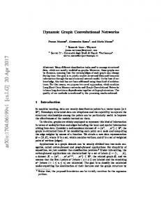
Figure 1: Left illustrates Alexnet filters. Middle shows Gabor filters. Right presents the convolution filters modulated by Gabor filters. Filters are often redundantly learned in CNN, and some of which are similar to Gabor filters. From this fact, we are motivated to actively manipulate the learned filters using Gabor filters, and consequently the number of learned filters can be reduced and leading to a compressed deep model. In the right column, a filter is modulated by Gabor filters via Eq. 2 to enhance the orientation property. scalable and end-to-end model has the amazing capability of learning powerful feature representations from raw pixels, boosting performance of many computer vision tasks, such as image classification, object detection, and semantic segmentation. Unlike hand-crafted filters without any learning process, DCNNs-based feature extraction is a purely data-driven technique that can learn robust representations from data, but usually at the cost of expensive training and complex model parameters. Additionally, the capability of modeling geometric transformations mostly comes from extensive data augmentation, large models, and handcrafted modules (e.g., max-pooling [1] for small translation-invariance). Therefore, DCNNs normally fail to handle large and unknown object transformations if the training data are not enough, one reason of which originates from the way of filter designing [1, 26]. Fortunately, the need to enhance model capacity to transformations has been perceived by researchers and some attempts have been made in recent years. In [3], a deformable convolution filter was introduced to enhance DCNNs’ capacity of modeling geometric transformations. It allows free form deformation of the sampling grid, whose offsets are learned from the preceding feature maps. However, the deformable filtering is still complicated and associated with the RoI pooling technique originally designed for object detection [5]. In [26], Actively Rotating Filters (ARFs) was proposed to give DCNNs the generalization ability of rotation. However, such a filter rotation method is actually only suitable to small and simple filters, i.e., with sizes of 1x1 and 3x3. Though the authors claimed a general method to modulate the filters based on the Fourier transform, it was not implemented in [26]. One of the reasons may lie in its computational complexity. Furthermore, 3D filters [10] are hardly modified by deformable filters or ARFs. In [8], by combining low level filters (Gaussian derivatives up to the 4-th order) with learned weight coefficients, the regularization over the filter function space is shown to improve the generalization ability but only when the set of training data is small. In Fig. 1 the visualization of convolutional filters [12] indicates that filters are often redundantly learned, such as those Alexnet filters trained on ImageNet1 , and some of the filters from shallow layers are similar to Gabor filters. It is known that the steerable properties of Gabor filters dominate the traditional filter design due to their enhanced capability of scale and orientation decomposition of signals, which is unfortunately neglected in prevailing convolutional filters in DCNNs. Can we just learn a small set of filters, which are then manipulated to create more in a similar way as the design of Gabor filters? If so, one of the obvious advantages lies in that we just need to learn a small set of filters for DCNNs, leading to a more compact but enhanced deep model. 1 For

illustration purpose, Alexnet is selected because its filters are of big sizes.


3

In this paper we propose using traditional hand-crafted Gabor filters to manipulate the learnable convolution filters with the aim to reduce the number of learnable network parameters and enhance the deep features. The manipulation of learnable convolution filters with powerful Gabor filters produces convolutional Gabor orientation filters (GoFs), which endow the convolution filters the additional capability of capturing the visual properties such as spatial localization, orientation selectivity and spatial frequency selectivity in the output feature maps. GoFs are implemented on the basic element of CNNs, i.e., the convolution filter, and thus can be easily integrated into any deep architecture. DCNNs with GoFs, referred to as Gabor CNNs (GCNs), can learn more robust feature representations, particularly for images of spatial transformations. Owing to a set of steerable filters that can generate enhanced feature maps for Gabor CNNs, the resulting model is more compact and representative with a small set of learned filters, and thus is easy to train. The contributions of this paper are summarized as follows: 1) To the best of our knowledge, it is the first time Gabor filters are incorporated into the convolution filter to improve the robustness of DCNNs to image transformations such as transitions, scale changes and rotations. 2) Without bells and whistles, GCNs improve the widely used DCNNs architectures including conventional CNNs and ResNet [6], obtaining new state-of-the-art results on popular benchmarks.

2 2.1

Related Work Gabor filters

Gabor wavelets [4] were invented by Dennis Gabor using complex functions to serve as a basis for Fourier transforms in information theory applications. An important property of the wavelets is that the product of its standard deviations is minimized in both time and frequency domains. Gabor was widely used to model receptive fields of simple cells of the visual cortex. The Gabor wavelets (kernels or filters) are defined as follows [17]: Ψu,v (z) =

||ku,v ||2 −(||ku,v ||2 ||z||2 /2σ 2 ) iku,v z 2 e [e − e−σ /2 ] σ2

(1)

√ (v−1) where ku,v = kv eiku , kv = (π/2)/ 2 , ku = u Uπ , with v = 0, ...,V and u = 0, ...,U and v is the frequency and u is the orientation, and σ = 2π. In [19, 25], Gabor wavelets were used to initialize the deep models or serve as the input layer. However, we take a different approach by utilizing Gabor filters to modulate the learned convolution filters. Specifically, we change the basic element of CNNs – convolution filters to GoFs to enforce the impact of Gabor filters on each convolutional layer. Therefore, the steerable properties are inherited into the DCNNs to enhance the robustness to scale and orientation variations in feature representations.

2.2

Learning feature representations

Given rich and often redundant convolutional filters, data augmentation is used to achieve local/global transform invariance [22]. Despite the effectiveness of data augmentation, the main drawback lies in that learning all possible transformations usually requires a lot of network parameters, which significantly increases the training cost and the risk of over-fitting.

4


Most recently, TI-Pooling [13] alleviates the drawback by using parallel network architectures for the transformation set and applying the transformation invariant pooling operator on the outputs before the top layer. Nevertheless, with a built-in data augmentation, TI-Pooling requires significantly more training and testing computational cost than a standard CNN. Spatial Transformer Networks: To gain more robustness against spatial transformations, a new framework for spatial transformation termed spatial transformer network (STN) [9] is introduced by using an additional network module that can manipulate the feature maps according to the transform matrix estimated with a localisation sub-CNN. However, STN does not provide a solution to precisely estimate complex transformation parameters. Oriented Response Networks: By using Actively Rotating Filters (ARFs) to generate orientation-tensor feature maps, Oriented Response Network (ORN) [26] encodes hierarchical orientation responses of discriminative structures. With these responses, ORN can be used to either encode the orientation-invariant feature representation or estimate object orientations. However, ORN is more suitable to small size filters, i.e., 3x3, whose orientation invariance property is not guaranteed by the ORAlign strategy based on their marginal performance improvement as compared with TI-Pooling. Deformable convolutional network: Deformable convolution and deformable RoI pooling are introduced in [3] to enhance the transformation modeling capacity of CNNs, making the network robust to geometric transformations. However, the deformable filters still prefer operating on small-sized filters. Scattering Networks: In wavelet scattering network [2, 20], expressing receptive fields in CNNs as a weighted sum over a fixed basis allows the new structured receptive field networks to increase the performance considerably over unstructured CNNs for small and medium datasets. In contrast to the scattering networks, our GCNs are based on Gabor filters to change the convolution filters in a steerable way.

3

Gabor CNNs

Gabor Convolutional Networks (GCNs) are deep convolutional neural networks using Gabor orientation filters (GoFs). An GoF is a steerable filter, created by manipulating the learned filters via Gabor filter banks, and then used to produce the enhanced feature maps. With GoFs, GCNs ont only involve significant fewer learnable filters and thus are easy to be trained, but also lead to enhanced deep models. In what follows, we address three issues in adopting GoFs in DCNNs. First, we give the details on obtaining GoFs through Gabor filters. Second, we describe convolutions that use GoFs to produce feature maps with scale and orientation information enhanced. Third, we show how GoFs are learned during the back-propagation update stage.

3.1

Convolutional Gabor orientation Filters (GoFs)

Gabor filters are of U directions and V scales. To incorporate the steerable properties into the GCNs, the orientation information is encoded in the learned filters, and at the same time the scale information is embedded into different layers. Due to the orientation and scale information captured by Gabor filters in GoFs, the corresponding convolution features are enhanced. Before being modulated by Gabor filters, the convolution filters in standard CNNs are learned by back propagation (BP) algorithm, which are denoted as learned filters. Let a

5

: GAOBR CONVOLUTION NETWORKS GCConv

Learned filter 4x3x3

Gabor filter bank 4, 3x3

Input feature map (F)

GoF 4x4x3x3

1x4x32x32

GoF 4x4x3x3

Onput feature map (Fˆ ) 1x4x30x30

Figure 2: Left shows modulation process of GoFs. Right illustrates an example of GCN convolution with 4 channels. In a GoF, the number of channels is set to be the number of Gabor orientations U for implementation convenience. learned filter be with size N × W × W , where W × W is the size of 2D filter (N channels). For implementation convenience, N is chosen to be U the number of the orientations of the Gabor filters that will be used to modulate this learned filter. A GoF is obtained based on a modulated process using U Gabor filters on the learned filters for a given scale v. The details concerning the filter modulation are shown in Eq. 2 and Fig. 2. For the vth scale, we define: v Ci,u = Ci,o ◦ G(u, v)

(2)

where Ci,o is a learned filter, and ◦ is an element-by-element product operation between v is the modulated filter of C by the v-scale Gabor G(u, v) 2 and each 2D filter of Ci,o . Ci,u i,o filter G(u, v). And a GoF is defined as: v v Civ = (Ci,1 , ...,Ci,U )

(3)

Thus, the ith GoF Civ is actually U 3D filters (see Fig. 2, here U = 4). In GoFs, the value of v increases with increasing layers, which means that scales of Gabor filters in GoFs are changed based on layers. At each scale, the size of a GoF is U × N × W × W . But we only save N ×W ×W -sized learned filters, because Gabor filters are given. To simplify the description of the learning process, v is omitted in the next section.

3.2

GCN convolution

In GCNs, GoFs are used to produce feature maps, which explicitly enhance the scale and orientation information in deep features. A output feature map Fb in GCNs is denoted as: Fb = GCconv(F,Ci )

(4)

where Ci is the ith GoF and F is the input feature map as shown in Fig. 2. The channels of Fb is obtained by the following convolution: N

Fbi,k =

(n)

∑ F (n) ⊗Ci,u=k

(5)

n=1

where (n) refers to the nth channel of F and Ci,u , and Fbi,k is the kth orientation response of b For example as shown in Fig. 2, let the size of the input feature map be 1 × 4 × 32 × 32. F. If there are 10 GoFs with 4 Gabor orientations, the size of the output feature map is 10 × 4 × 30 × 30. 2 Real

parts of Gabor filters are used

6

: GAOBR CONVOLUTION NETWORKS xl C: Spatial Convolution

CNN

MP: Max Pooling

Input image

C 3*3 80

1x32x32

R: ReLu

MP+R

M: Max

C 3x3 160

80*15*15

MP+R

Align: ORAlign C 3x3 320

MP+R

160*6*6

320*3*3

BN：BatchNormlization

C 3x3 160

R

FC

640*1*1

xl

GCN

Input image

Extend 4

1x32x32

1x4x32x32

Input image

Extend 4

1x32x32

1x4x32x32

ORConv4 4x3x3,20

MP +R

ORConv4 4x3x3,40

20x4x15x15

MP +R

ORConv4 4x3x3,80

40x4x6x6

MP +R

80x4x3x3

GC(4,v=1) B MP 4x3x3,20 N +R

GC(4,v=2) B MP 4x3x3,20 N +R

GC(4,v=3) B MP 4x3x3,20 N +R

20x4x15x15

40x4x6x6

80x4x3x3

ORConv4 4x3x3,160

R

160x4x1x1

D

1024*1

GC(4,v=4) B R 4x3x3,20 N

160x4x1x1

Align

160x4

FC

Output

Conv3x3

10*1

D

1024x1

M

FC

160x1

1024x1

3.3

5x5 1.86 0.48 0.48

5x5 0.51 0.57 0.56

3x3 0.78 0.51 0.49

3x3 0.25 0.7 0.63

GCConv5x5

GCConv3x3

GCConv3x3

Conv1x1

Output

10x1

D

+

+

+

+

xl+1

xl+1

xl+1

xl+1

Output

(b) Resnet bottleneck

(c) GCN basic-1

(d) GCN basic-2

10x1

Figure 3: Network structures of CNNs, ORNs and GCNs.

kernel # params (M) V = 1 scale V = 4 scales

GCConv3x3 Conv3x3

(a) Resnet basic block

Table 1: Results (error rate (%) on MNIST) vs. Gabor filter scales.

xl

Conv1x1

Conv3x3 ORN

xl

D:Dropout

Figure 4: The residual block. (a) and (b) are for ResNet. (c) Small kernel and (d) large kernel are for GCNs.

Table 2: Results (error rate (%) on MNIST) vs. Gabor filter orientations. U 5x5 3x3

2 0.52 0.68

3 0.51 0.58

4 0.48 0.56

5 0.49 0.59

6 0.49 0.56

7 0.52 0.6

Updating GoF

In the back-propagation (BP) process, only the leaned filer Ci,o needs to be updated. And we have: U ∂L δ=∑ (6) u=1 ∂Ci,u Ci,o = Ci,o − ηδ

(7)

where L is the loss function. From the above description, it can be seen that the BP process is easily implemented and is very different from ORNs and deformable kernels that usually require a relatively complicated procedure. By only updating the learned convolution filters Ci,o , the GCNs model can be more compact and efficient, and also is more robust to orientation and scale variations.

4

Implementation and Experiments

In this section, we present the details of the GCNs implementation based on conventional DCNNs architectures. Afterwards, we evaluate GCNs on the MNIST digit recognition dataset [14, 15] as well as its rotated version MNIST-rot used in ORNs, which is generated by rotating each sample in the MNIST dataset by a random angle between [0,2π]. To further evaluate the performance of GCNs, the experiments on the SVHN dataset [18], CIFAR-10 and CIFAR-100 [11] are also provided 3 . We have two GPU platforms used in our experiments, NVIDIA GeForce GTX 1070 and GeForce GTX TITAN X(2).

4.1

MNIST

For the MNIST dataset, we randomly select 10,000 samples from the training set for validation and the remaining 50,000 samples for training. Adadelta optimization algorithm [24] is 3

Please also refer to the supplementary materials for more details.

7

: GAOBR CONVOLUTION NETWORKS Bird Ship Deer 4.1% 2.5% 3.2%

Figure 5: Recognition results of different categories on CIFAR10. Compared with ResNet110, GCNs perform significantly better on the categories with large scale variation. Table 3: Results comparison on MNIST Baseline CNN STN TIPooling(×8) ORN4(ORAlign) ORN8(ORAlign) ORN4(ORPooling) ORN8(ORPooling) GCN4(with 3 × 3) GCN4(with 3 × 3) GCN4(with 5 × 5) GCN4(with 5 × 5) GCN4(with 7 × 7) GCN4(with 7 × 7)

Method # network stage kernels 80-160-320-640 80-160-320-640 (80-160-320-640)×8 10-20-40-80 10-20-40-80 10-20-40-80 10-20-40-80 10-20-40-80 20-40-80-160 10-20-40-80 20-40-80-160 10-20-40-80 20-40-80-160

# params (M) 3.08 3.20 24.64 0.49 0.96 0.25 0.39 0.25 0.78 0.51 1.86 0.92 3.17

time (s) 6.50 7.33 50.21 9.21 16.01 4.60 6.56 3.45 6.67 10.45 23.85 10.80 25.17

MNIST 0.73 0.61 0.97 0.57 0.59 0.59 0.66 0.63 0.56 0.49 0.48 0.46 0.42

error (%) MNIST-rot 2.82 2.52 not permitted 1.69 1.42 1.84 1.37 1.45 1.28 1.26 1.10 1.33 1.20

Table 4: Results comparison on SVHN. No additional training set is used for training Method # params Accuracy (%)

VGG 20.3M 95.66

ResNet-110 1.7M 95.8

ResNet-172 2.7M 95.88

GCN4-40 2.2M 96.9

GCN4-28 1.4M 96.86

ORN4-40 2.2M 96.35

ORN4-28 1.4M 96.19

used during the training process, with the batch size as 128, initial learning rate as 0.001 (η) and weight decay as 0.00005. The learning rate is reduced to half per 25 epochs. We report the performance of our algorithm on a test set after 200 epochs based on the average over 5 runs. The state-of-the-art STN [9], TI-Pooling [13], ResNet [6] and ORNs [26] are involved in the comparison. Among them, STN is more robust to spatial transformation than the baseline CNNs, due to a spatial transform layer prior to the first convolution layer. TI-Pooling adopts a transform-invariant pooling layer to get the response of main direction, resulting in rotation robust features. ORNs capture the response of each direction by rotating the original convolution kernel spatially. Fig. 3 shows the network structures of CNNs, ORNs and GCNs (U = 4), which are used in this experiment. For all models, we adopt Max-pooling and ReLU after convolution layers, and a dropout layer [7] after FC layer to avoid over-fitting. To compare with other CNNs in a similar model size, we reduce the width of layer 4 by a certain proportion as done 4 The

number of convolution kernels per layer.

8


Table 5: Results comparison on CIFAR-10 and CIFAR-100 error (%) CIFAR-10 CIFAR-100 8.81 35.67 6.32 28.49

Method NIN VGG # network stage kernels ResNet-110 ResNet-1202 GCN2-110 GCN2-110 GCN4-110 GCN2-40 GCN4-40 WRN-40 WRN-28 GCN2-40 GCN4-40 GCN3-28

16-16-32-64 16-16-32-64 12-12-24-45 16-16-32-64 8-8-16-32 16-32-64-128 16-16-32-64 64-64-128-256 160-160-320-640 16-64-128-256 16-32-64-128 64-64-128-256

# params Fig.4(c)/Fig.4(d) 1.7M 10.2M 1.7M/3.3M 3.4M/6.5M 1.7M 4.5M 2.2M 8.9M 36.5M 17.9M 8.9M 17.6M

6.43 7.83 6.34/5.62 5.65/4.96 6.19 4.95 5.34 4.53 4.00 4.41 4.65 3.88

25.16 27.82 26.14/25.3 24.23 25.65 21.18 19.25 20.73 21.75 20.13

in ORNs, i.e., 1/8 [26]. We evaluate different scales for different GCNs layers (i.e., V = 4,V = 1), where larger scale Gabor filters are used on shallow layers or a single scale is used on all layers. It should be noted that in the following experiments, we also use V = 4 for deeper networks (ResNet), which are equally distributed across layers. As shown in Table 1, the results of V = 4 in terms of error rate are better than those when a single scale (V = 1) is used on all layers when U = 4. We also test different orientations as shown in Table 2. The results indicate that GCNs perform better using 3 to 6 orientations when V = 4, which is more flexible than ORNs. In comparison, ORNs use a complicated interpolation process via ARFs besides 4and 8-pixel rotations. In Table 3, the second column refers to the width of each layer, and a similar notation is also used in [23]. Considering a GoF has multiple channels (N), we decrease the width of layer (i.e., the number of GoFs per layer) to reduce the model size for the purpose of a fair comparison. The parameter size of GCNs is linear with channel (N) but quadratic with width of layer. Therefore, the GCNs complexity is reduced as compared with CNNs (see the third column of Table 3). In the fourth column, we compare the computation time (s) for training epoch of different methods using GTX 1070, which clearly shows that GCNs are more efficient than other state-of-the-art models. The performance comparison is shown in the last two columns in terms of error rate. By comparing with baseline CNNs, GCNs achieved much better performance with 3x3 kernel but only using 1/12, 1/4 parameters of CNNs. It is observed from experiments that the GCNs with 5x5 and 7x7 kernels achieve 1.10% on MNIST-rot and 0.42% on MNIST test error respectively, which are better than those of ORNs. This can be explained by the fact that the kernels with larger size carry more information of Gabor orientation, and thus capture better orientation response features. Table 3 also demonstrates that a larger GCN model can result into a better performance. In addition, in MNIST-rot datasets, the performance of baseline CNN model is greatly disturbed by rotation, while ORNs and GCNs can capture orientation features and achieve better results. Again, GCNs outperform than ORNs, which confirms that Gabor modulation indeed helps to gain the robustness to the rotation variations, because deep features are enhanced based on steerable filters. In contrast, ORNs just actively rotate the filters and lack a feature


9

enhancement process.

4.2

SVHN

The Street View House Numbers (SVHN) dataset [18] is a real-world image dataset taken from Google Street View images. SVHN contains MNIST-like 32x32-sized images centered around a single character, which however include a plethora of challenges like illumination changes, rotations and complex backgrounds. The dataset consists of 600000 digit images: 73257 digits for training, 26032 digits for testing, and 531131 additional images. Note that the additional images are not used for all methods in this experiment. For this large scale dataset, we implement GCNs based on ResNet. Specifically, we replace the spatial convolution layers with our GoFs based GCConv layers, leading to GCN-ResNet. The bottleneck structure is not used since the 1x1 kernel does not propagate any Gabor filter information. ResNet divides the whole network into 4 stages, and the width of stage (the number of convolution kernels per layer) is set as 16,16,32,64, respectively. We make appropriate adjustments to the network depth and width to ensure our GCNs method has a similar model size as compared with VGG [21] and ResNet. And we set up 40-layer and 28-layer GCN-ResNets with basic block-(c)(Fig. 4), using the same hyper-parameters as ResNet. The network stage is also set as 16-16-32-64. The results are shown in Table 4. Compared to VGG model, GCNs have much smaller parameter size, yet obtain a better performance with 1.2% improvement. With a similar parameter size, the GCN-ResNet achieves better results (1.1%, 0.66%) than ResNet and ORNs respectively, which further validates the superiority of GCNs for realworld problems.

4.3

Natural Image Classification

For the natural image classification task, we use the CIFAR datasets including CIFAR-10 and CIFAR-100 [11]. The CIFAR datasets consist of 60000 32x32-sized color images in 10 or 100 classes, with 6000 or 600 images per class. There are 50000 training images and 10000 test images. CIFAR datasets contain a wide variety of categories with object scale and orientation variations. Similar to SVHN, we test GCN-ResNet on CIFAR datasets. Experiments are conducted to compare our method with the state-of-the-art networks (i.e., NIN [16], VGG [21], ORN [26] and ResNet [6]). For example on CIFAR-10, Table 5 shows that GCNs consistently improve the performance regardless of the number of parameters or kernels as compared with baseline ResNet. We further compare GCNs with Wide Residue network (WRN) [23], and again it achieves a better performance (4% vs. 3.88%) when our model is half the size of WRN, indicating significant advantage of GCNs in terms of model efficiency. Similar to CIFAR-10, one can also observe the performance improvement on CIFAR-100, with similar parameter sizes. Moreover, when using different kernel size configurations (from 3 × 3 to 5 × 5 as shown in Fig. 4(c) and Fig. 4(d)), the model size is increased but with a performance (error rate) improvement from 6.34% to 5.62%. We notice that some top improved classes in CIFAR10 are bird (4.1% higher than baseline ResNet), and deer (3.2%), which exhibit significant within class scale variations. This implies that the Gabor manipulation in CNNs enhances the capability of handling scale variations as shown in Fig. 5.

10

5


Conclusion

This paper has incorporate Gabor filters to DCNNs, aiming to enhance the deep feature representations with steerable orientation and scale capacities. The proposed Gabor Convolutional Networks (GCNs) improve DCNNs on the generalization ability of rotation and scale variations by introducing extra functional modules on the basic element of DCNNs, i.e., the convolution filters. GCNs can be easily implemented using popular architectures. The extensive experiments show that GCNs significantly improved baselines, resulting in the state-of-the-art performance over several benchmarks.

References [1] Y-Lan Boureau, Jean Ponce, and Yann LeCun. A theoretical analysis of feature pooling in visual recognition. In Proceedings of the 27th international conference on machine learning (ICML), pages 111–118, 2010. [2] Joan Bruna and Stéphane Mallat. Invariant scattering convolution networks. IEEE transactions on pattern analysis and machine intelligence, 35(8):1872–1886, 2013. [3] Jifeng Dai, Haozhi Qi, Yuwen Xiong, Yi Li, Guodong Zhang, Han Hu, and Yichen Wei. Deformable convolutional networks. arXiv preprint arXiv:1703.06211, 2017. [4] Dennis Gabor. Theory of communication. part 1: The analysis of information. Journal of the Institution of Electrical Engineers-Part III: Radio and Communication Engineering, 93(26):429–441, 1946. [5] Ross Girshick. Fast r-cnn. In Proceedings of the IEEE International Conference on Computer Vision, pages 1440–1448, 2015. [6] Kaiming He, Xiangyu Zhang, Shaoqing Ren, and Jian Sun. Deep residual learning for image recognition. In Proceedings of the IEEE Conference on Computer Vision and Pattern Recognition, pages 770–778, 2016. [7] Geoffrey E Hinton, Nitish Srivastava, Alex Krizhevsky, Ilya Sutskever, and Ruslan R Salakhutdinov. Improving neural networks by preventing co-adaptation of feature detectors. arXiv preprint arXiv:1207.0580, 2012. [8] Jorn-Henrik Jacobsen, Jan van Gemert, Zhongyu Lou, and Arnold WM Smeulders. Structured receptive fields in cnns. In Proceedings of the IEEE Conference on Computer Vision and Pattern Recognition, pages 2610–2619, 2016. [9] Max Jaderberg, Karen Simonyan, Andrew Zisserman, et al. Spatial transformer networks. In Advances in Neural Information Processing Systems, pages 2017–2025, 2015. [10] Shuiwang Ji, Wei Xu, Ming Yang, and Kai Yu. 3d convolutional neural networks for human action recognition. IEEE transactions on pattern analysis and machine intelligence, 35(1):221–231, 2013. [11] Alex Krizhevsky and Geoffrey Hinton. Learning multiple layers of features from tiny images. 2009.


11

[12] Alex Krizhevsky, Ilya Sutskever, and Geoffrey E Hinton. Imagenet classification with deep convolutional neural networks. In Advances in neural information processing systems, pages 1097–1105, 2012. [13] Dmitry Laptev, Nikolay Savinov, Joachim M Buhmann, and Marc Pollefeys. Tipooling: transformation-invariant pooling for feature learning in convolutional neural networks. In Proceedings of the IEEE Conference on Computer Vision and Pattern Recognition, pages 289–297, 2016. [14] Yann LeCun, Léon Bottou, Yoshua Bengio, and Patrick Haffner. Gradient-based learning applied to document recognition. Proceedings of the IEEE, 86(11):2278–2324, 1998. [15] Yann LeCun, Corinna Cortes, and Christopher JC Burges. The mnist database of handwritten digits, 1998. [16] Min Lin, Qiang Chen, and Shuicheng Yan. Network in network. in Proc. of ICLR, 2014. [17] Chengjun Liu and Harry Wechsler. Gabor feature based classification using the enhanced fisher linear discriminant model for face recognition. IEEE Transactions on Image processing, 11(4):467–476, 2002. [18] Yuval Netzer, Tao Wang, Adam Coates, Alessandro Bissacco, Bo Wu, and Andrew Y Ng. Reading digits in natural images with unsupervised feature learning. In NIPS workshop on deep learning and unsupervised feature learning, volume 2011, page 5, 2011. [19] Wanli Ouyang and Xiaogang Wang. Joint deep learning for pedestrian detection. In Proceedings of the IEEE International Conference on Computer Vision, pages 2056– 2063, 2013. [20] Laurent Sifre and Stéphane Mallat. Rotation, scaling and deformation invariant scattering for texture discrimination. In Proceedings of the IEEE conference on computer vision and pattern recognition, pages 1233–1240, 2013. [21] Karen Simonyan and Andrew Zisserman. Very deep convolutional networks for largescale image recognition. arXiv preprint arXiv:1409.1556, 2014. [22] David A Van Dyk and Xiao-Li Meng. The art of data augmentation. Journal of Computational and Graphical Statistics, 10(1):1–50, 2001. [23] Sergey Zagoruyko and Nikos Komodakis. Wide residual networks. arXiv preprint arXiv:1605.07146, 2016. [24] Matthew D Zeiler. Adadelta: an adaptive learning rate method. arXiv:1212.5701, 2012.

arXiv preprint

[25] Zhuoyao Zhong, Lianwen Jin, and Zecheng Xie. High performance offline handwritten chinese character recognition using googlenet and directional feature maps. In 13th International Conference on Document Analysis and Recognition (ICDAR), pages 846– 850. IEEE, 2015.

12


[26] Yanzhao Zhou, Qixiang Ye, Qiang Qiu, and Jianbin Jiao. Oriented response networks. Proceedings of the Internaltional Conference on Computer Vision and Pattern Recogintion, 2017.