Gabor Wavelets for 3-D Object Recognition Xing Wu and Bir Bhanu College of Engineering University of California, Riverside, CA 92521-0425 Email: xingwu@constitution .ucr.edu,
[email protected] .edu 2
Abstract This paper presents a model-based object recognition approach that uses a hierarchical Gabor wavelet representation. The key idea is to use magnitude, phase and frequency measures of Gabor wavelet representation in a n innovative flexible matching approach that can provide robust recognition. A Gabor grid, a topology-preserving map, eficiently encodes both signal energy and structural information of an object in a sparse multi-resolution representation. T h e Gabor grid subsamples the Gabor wavelet decomposition of a n object model and is deformed to allow the indexed object model match with the image data. Flexible matching between the model and the image minimizes a cost function based on local similarity and geometric distortion of the Gabor grid. Grid erosion and repairing is performed whenever a collapsed grid, due to object occlusion, is detected. T h e results o n infrared imagery are presented, where objects undergo rotation, translation, scale, occlusion and aspect variations under changing environmental conditions.
1
Our Approach
The general scheme of our system is depicted in Figure 1. It is implemented as a n iterative process of matching by first finding the optimal global placement of t h e grid over a regionof-interest of the object while the grid is kept rigid (location indexing), then deformation of the grid allows model Gabor probes match with local features of the distorted image (flexible matching). Gabor magnitude is used in probe matching based on local structural energy patterns. Gabor frequency is used to estimate the scale variation of a given object from the model. Gabor phase is used t o evaluate t h e matching result in terms of average local image displacement between the model and the data, and support interpolation between aspects of the model. In our work, 3 0 objects are represented by a series of viewer-centered 2 0 images of the objects at various aspect and depression angles, M = { M I ,M z , . . . ,M K } , called object aspects. These models are generated offline. Both object and object model are represented by t h e magnitude and
Introduction
--
Model-based object recognition in real-world outdoor situations is difficult because a robust algorithm has t o consider multiple factors such as, object contrast, signature, scale, and aspect variations; noise and spurious low resolution sensor data; and high clutter, partial object occlusion and articulation. Current approaches use shape primitives, silhouette and contours, colors, and invariant object features for matching. The performance of these methods is acceptable when objects are well defined, have high contrast, and are at close ranges. However, these approaches do not gracefully degrade and produce high false alarms when competitive clutter and object shape distortion are present in the input data. To improve the performance under multi-scenarios and varying environmental conditions, model of sensors, atmosphere, and background clutter are helpful in addition t o the geometric model of a n object. Using only a minimum set of models and sensor model, multi-scale Gabor representation and a flexible matching mechanism described in the paper can help to improve the recognition performance under real-world situations. The goal of the research presented in this paper is to recognize 3 0 rigid objects in cluttered multisensor images with varying appearances, signatures and possible partial occlusion using a model-based paradigm.
Object Image
meavures for indexing
I I
b) Grid Repainng
Object Class and P m e
Figure 1: Our object recognition approach.
537
I I I I
phase responses of multi-scale Gabor wavelet filters. Objects are recognized when they successfully match with a specific model based on distinctive local features in the Gabor wavelet representation. The most closely related work to our approach is Lades’s “Dynamic Link Architecture” technique (41. The key differences between our approach and Lades’s techniques are given in [l]. The main contribution of this paper is to use Gabor wavelet representation to recognize 3-D objects under scale, aspect and significant distortions in shape and appearance, due to changing environmental conditions.
2.1
Gabor F‘unction and Gabor Wavelets
The general form of a 2 0 Gabor function is given as [2],
Figure 2: Gabor probe and grid
+
+
grid, xJ = (20 nDspaceryo m D s p a c e ) PJ . is a vector of length K x L which is referred to as a Gabor probe,
p:[k, l1
=
( I * G;k,t)[xJ],
1‘
=
(I * GGk,t)[xJl.
‘J-[’?
In the above formula, ( x , , y , ) is the spatial centroid of the elliptical Gaussian window whose scale and aspect are regulated by u and a,respectively. W k and 61 are the modulation frequency and direction, and (U,U ) are frequency components of W k in x and y directions, respectively. The scale u controls the size of the filter as well as its bandwidth, while the aspect ratio a and the rotation parameter +G control the shape of the spatial window and the spectral channel passband and is generally set equal to 61. By representing Gabor wavelet filters as a propagated quadrature pair ( G$ , G , ), a representation which is similar to the so called wavelet [5] is defined. The log-polar sampling in the freque_ncy domain generated by the 2 0 wave propagation vector is given as:
+
&,,k,e,
= wli.eref, where
Wk
Therefore, the wavelet filter kernel’s frequency and orientation bandwidth are defined as: hWk
=X W ~ ,
where (G$&.,, G , , , ) is a Gabor wavelet quadrature filter pair with center frequency W & and modulation orientation + l . The role of the graph edges e,,J E Enis to represent neighborhood relationships and serve as constraint during matching, where they are interpreted as elastic links. An edge can be deformed like a spring to make a model probe match with the Gabor decomposition of a distorted object. The length between two nodes d,, = 111, - x,I) and grid angle attached to that edge serve as initial constraints. Thus, current distortions can be measured and penalized immediately during matching. Figure 2 shows the Gabor grid and Gabor probe representation. The extracted information (both signal energy and local pattern structure) associated with each probe spans a neighborhood whose size equals the extent of the filter kernel.
3
= pk.wo, and 81 = 1 . 6 0 . (2)
Also, the modulation frequency increases proportionally with the reduction in scale,
A6i
%
A.
(4)
whereX is called bandwidth-frequency ratio. The Gabor wavelet decomposition of an object image I ( x ) is an iconic multi-resolution template. To reduce the interpixel redundancy, subsampling this template forms an elastic Gabor grid GD which covers the whole object with N x M nodes (vertices V , and edges E J ) in the x and y directions, respectively, GD = (V,, En). Each node V k E V, is a triple, vJ = ( x 3 ,P:, P;) where x3 is the image coordinates of grid node j (with respect to some normalized coordinate frame). Nodes are selected with fixed distance Dspocefrom neighboring nodes for a model
(5)
Object Recognition-Flexible Matching
The flexible matching for object recognition process includes (1) Grid placement to find the location and index of an object in an input image; (2) Flexible matching to fine tune the object aspect according to the object distortion present in the input data; and (3) Evaluation to select the best matched aspect by following the selected rules. Grid repairing is performed when object is occluded.
3.1
Location Indexing
At this stage of the matching process, the indexed aspect Gabor grid G I & that potentially corresponds to the object aspect At& is positioned ( X & ) , scaled (st&), and rotated (4&), according to the index elements while the grid is kept rigid,
where
538
for all U, E V,dz and e,,] E E,ds. The function S 5 , @performs () scaling and rotation operations on the grid nodes. When the scale factor s is a power of W O and the orientation d is a multiple of 40,it corresponds to deriving a new model grid Gb at a given scale by scaling down edges of the Gabor grid by factor s. and shifting and rotating Gabor probe PI at each node vl from the corresponding frequency index wJ and orientation c$+,
In case s is not a multiple of p or 9 is a not a power of A,, we can either, (a) round the scale factor s to s’ which is the closest multiple of the frequency index p in ( 7 ) , and let the subsequent flexible matching overcome this small scale distortion in Gabor decomposition. However, the grid edge will be scaled according to the exact scale factor s. or, (b) implement a suitable interpolation scheme over scale and orientation. The object decomposition by a Gabor filter at a specific frequency corresponds to an object representation a t a specific scale. By comparing the similarities of these representations between an object and a model grid, it allows to estimate the object scale.
3.2
pV2u
(c) Matching result
(d) Projected model
2. For each grid node (visited in random order), take a random step s. A move s for a node is valid and can be accepted if either,
-
the global cost C is reduced due to this move, or - AC satisfies a probability exp(-AC/T), where T is the annealing temperature.
3. The matching terminates and produces a deformed model grid if either the matching reaches a desired cost, or the annealing temperature is freezing. If neither condition is satisfied, continue previous step with temperature decreased by a cooling factor 8. 4. Compute the similarity between the distorted model grid and the object Gabor decomposition, the deformation of the model grid, and the Gabor phase-based matching error (see section 3.5).
To show the quality of flexible matching under distortions, an example is given in Figure 3, in which a matched model is back projected onto the object image using the transformation which is calculated based on the relationship between the model grid and the matched deformed grid, and bilinear interpolation for gray scale values. The pose of the object is also derived in this manner.
f3U
+ (Y + p ) + F = 0, ax
where x is the coordinate of the object, U is the displacement of the deformation, F is the external forces, and /I and y define the elastic properties of the object. To find the equilibrium state when the deformable model grid is matched with an object decomposition, equation (8) is formatted as an iterative process which minimizes a cost function C balanced between grid distortions V and local similarities S . Therefore, we can rewrite (8) as following, N
(b) Object image
Figure 3: Illustration of the quality of flexible matching
Flexible Model Matching
After location indexing, flexible matching starts to further verify the hypothesis for a model aspect by moving nodes of the model Gabor grid locally and independently to find the best matched image probes. In this process, the 2 0 images of an object corresponding to two viewing aspects (with small aspect difference) is simulated by “small local” elastic deformations of one of the objects. When the external forces are applied, an elastic object is deformed until an equilibrium state between the external forces and internal forces resisting the deformation is achieved. This equilibrium state can be described as,
(a) Model image
3.3
Evaluation of Matching
The process of matching always yields a best value for C in (9) regardless of whether or not a corresponding object is in the model database. Successful recognition tends to have small geometric distortions and high similarity measurements. However, a matching result for the correct object class may not be distinctive when large object aspect variations and large changes in object signatures are present in the input data. To overcome the drawbacks of using only a single evaluation criterion, we introduce a set of comprehensive measures.
N
I
where N is the total number of grid nodes, p is the elastic parameter which controls the grid deformation. U, is a grid vertex, and PI and P M are the object Gabor decomposition and a model Gabor probe, respectively. D ’ and S are defined by equation (12) and (13), respectively.
1. Flexible matchzng cost c : It is given by ( Q ) , < combines the similarity measure between probes and grid distortions. To suppress background probes and compensate for grid deformation, the similarity measure term is mul-
Flexible Matching Algorithm 1. Use the index generated by the grid-placement algorithm as the initial placement of the model grid.
539
tiplied by the minimum magnitude of either the model or the object probe.
Dissimilarity E : It is defined as the difference between perfect matching and the actual matching results. E is zero for perfectly matched probes, and is less than 0.5 for a randomly matched probe pair. N E
=
[l -S(Pt', P;",]2
, I'
I
where
s is given by equation (13)
Figure 4: Illustration of grid deformation
Displacement 6 : It is defined as the local translational displacement between matched Gabor probes. Given that a model probe P, matches with an image probe P,, the localized phase difference along the direction of modulation t$1 for a specific filter frequency W k can be used to estimate this displacement and evaluate the matching error, A @ ( W k l t$r ) d ( W k , 41) = Wk (11) To find the correct object aspect after flexible matching, the results are evaluated based on the three criteria discussed above and the following rules in order. 1. For all matching results, sort the
e,
E
and delta in de-
scending order.
2. Select the model having both the lowest matching cost c and the smallest dissimilarity E . If neither the values of c or E for the top two matched models are distinguishable enough (by a predefined threshold), go to Step 4. 3. Select the model having the smallest dissimilarity E while its matching cost c and dissimilarity E are both lower than a predefined threshold.
comparing the current grid with its original structure which has fixed length and a rectilinear grid. The distortion for a node V k is then calculated as:
,=O
1=0
The first term in (12) measures the grid length distortion, while the second term measures the angular distortion. Given each Gabor probe as a vector of Gabor wavelet decomposition of magnitude at a spatial location, to match local features between two objects corresponds a search of maximum similarity between a model Gabor probe and an image probe. The similarity between two Gabor probes is computed as follow:
where q is a normalization term that is used to reduce the effect of object signature variations. In practice, we choose q to be the following:
4. Select the model having the smallest displacement measure which is less than a predefined threshold.
5. Any matches which fail the above tests are rejected for recognition. In a separate experiment to recognize 138 objects [l],a success rate of 61.8% was achieved when only the flexible matching cost is used in matching. The performance is improved by using other evaluation criteria, and a successful recognition rate of 98% was achieved when the three described evaluation criteria are used together (see Table 1).
Images
Criteria C ~~