PREPRINT with corrections. Presented at COMPSTAT, Invited Session on Image Analysis. Rome, Italy, August 2006.
Robust Correspondence Recognition for Computer Vision ˇara Radim S´ Center for Machine Perception, Department of Cybernetics Czech Technical University, Prague, Czech Republic
[email protected] Summary. In this paper we introduce a new robust framework suitable for the task of finding correspondences in computer vision. This task lies in the heart of many problems like stereovision, 3D model reconstruction, image stitching, camera autocalibration, recognition and image retrieval and a host of others. If the problem domain is general enough, the correspondence problem can seldom employ any well-structured prior knowledge. This leads to tasks that have to find maximum cardinality solutions satisfying some weak optimality condition and a set of constraints. To avoid artifacts, robustness is required to cope with decision under occlusion, uncertainty or insufficiency of data and local violations of prior model. The proposed framework is based on a robust modification of graph-theoretic notion known as digraph kernel.
Key words: computer vision, robust matching, digraph kernel
1 Introduction In computer vision there are many complex decision tasks where a suitable prior model has only a weak form. These tasks mostly involve correspondence recognition in general scenes. Given two or more images, the goal is to recognize which features in the target image(s) correspond to the features in the reference image. We mention the two most important here: the WideBaseline Stereo and the Semi-Dense Stereo since their character and their solution covers most of the other cases as well. In its simplest form the goal of Wide-Baseline Stereo is to recognize correspondences between the set of interest points in the reference and the target images. The images can be taken from very different viewpoints and possibly over long time periods. The usual first step involves finding a set of interest points in each image independently. These points are chosen to be well localized and stable under allowed image transformations [M+05]. A local image descriptor is then used to capture the content of the image neighborhood of
2
ˇara R. S´
each interest point [MS05]. The descriptor has to be invariant or at least insensitive to image deformation due to re-projection. Locality of descriptors is important for correspondence recognition in the presence of partial occlusion, time-induced image degradation factors, illumination changes, etc. Let A and B be the interest point sets including their description in the reference and target image, respectively. The computational problem is to find the largest partial one-to-one mapping M : A → B that has high probability and such that the epipolar condition is satisfied. The cardinality of the mapping is not known a priori. The condition has a parametric form x> B F xA = 0,
(1)
where xA (xB ) is the image location of an interest point in A (B, respectively) expressed in homogeneous representation (it is a 3-vector) and F is a homogeneous 3 × 3 fundamental matrix of rank 2. The constraint (1) predicts that the corresponding point xB must lie on the line FxA in the target image. The constraint has 7 independent parameters. See [HZ03] for more details on geometric constraints related to projective cameras. The standard, almost exclusively used solution to the wide baseline stereo (WBS) problem is robust fitting of (1) by RANSAC [FB81, HZ03]. The WBS problem has applications in camera autocalibration, image stitching, recognition and image retrieval, visual tasks for robotic manipulation and navigation, range image registration, etc. In Semi-Dense Stereo, the interest points are the set of all image points. The goal is similar as above, with some simplifications that allow introducing additional models. Based on the fundamental matrix F obtained from the WBS correspondences it is possible to transform the image domain so that the corresponding point in the target image is located on the same line as in the reference image. After the transformation the parametric constraint (1) is no longer required. The image transformation not only means it is not necessary to search the whole image for a correspondence but also eases the use of some useful constraints: It has been observed [YP84] that in a wide class of scenes the left-to-right order in which interest points occur in the reference image is preserved in their respective matching points in the other image. This means that the mapping M has a monotonicity property which is called the ordering constraint. Many different algorithms have been proposed that attempt to solve the semi-dense stereo problem, see [SS02] for a partial review. The semi-dense stereo problem has most applications in 3D modeling from images, in view synthesis, or in camera-based robotic obstacle avoidance. Of course, the problem of occlusion remains in semi-dense stereo. Occlusion means a surface point is visible in one image but it is occluded by another surface in the other image. We say a world point w (a point on surface or in midair) is ruled out by a binocularly visible point p if either w is occluded by p in one of the cameras or if w is in front of p in one of the cameras. The
Robust Correspondence Recognition
3
t3
occluded t1
surfaces
surface t2
X2 X1 X
transparent r1
(a)
(b) half occlusion
(c) mutual occlusion
Fig. 1. Occlusion: The surface point at the intersection of rays r1 and t1 (black) occludes a world point at the intersection (r1 , t3 ) and implies the world point (r1 , t2 ) is transparent, hence (r1 , t3 ) and (r1 , t2 ) are ruled-out by (r1 , t1 ) (a). In half-occlusion, every world point such as X1 or X2 is ruled out by a binocularly visible surface point (b, black dots). In mutual occlusion this is no longer the case (c, gray region).
situation is illustrated in Fig. 1. From algorithmic point of view, there are two fundamental types of occlusion: 1. Half-occlusion: the set of surface points visible to both cameras rules-out all other world points. This case is illustrated in Fig. 1(b). 2. Mutual occlusion: there are world points (in midair) that are not ruledout by surface points visible to both cameras. This case is illustrated in Fig.1(c). Once the slit becomes wide enough for the background surface to enter the zone, the zone shrinks or disappears (if ordering is to hold). Occlusion, mutual occlusion in particular, means we do not know a priori how large portion of the images can be interpreted as occluded or matched. It is clear that the unknown or unconstrained cardinality of the solution poses a serious problem in these tasks: The goal is not only to find a matching but also determine which of the interest points are to be discarded. Of course one should discard as little as possible but prior knowledge useful for such disposal is hard if not impossible to obtain. With the exception of [GY05, Sar02], none of the known algorithms models occlusion properly and exhibits the ability to reject part of input data that is required here. Repeated or constant appearance makes the problem worse: if the scene is a collection of small particles floating in the air, no local decision can determine which of the dots in the target image matches a particular dot in the reference image. The decision problem is somewhat easier if more than three cameras view the scene, especially if it is known that the scene consists of a surface visible to all cameras (i.e. when there are no occlusions) [BSK01]. Similarly, if a portion of the scene has constant appearance (consider a perfectly white wall), unique solution does not exist regardless of the number of cameras viewing it. Hence, one needs a degree of certainty that the result of solving the problem is correct, especially in the case when data do not suffice for unique deci-
4
ˇara R. S´
left image
right image
(a)
(b)
MAP via DP
Stable via GK
Fig. 2. Local invalidity of prior model and illusions. Left-image disparity maps colorcoding depth are obtained from two different algorithms (a,b). Gray in (a) means ‘occluded,’ in (b) it means ‘occluded or unexplained,’ the two are not distinguished to preserve clarity of the resulting picture. Both dynamic programming (DP) and the proposed graph kernel (GK) algorithm process image rows independently.
sion and/or under the presence of occlusion: Part of data must be rejected and the necessary component of the problem solution is therefore robustness. With the notable exception of RANSAC solution to the WBS problem, standard methods do not possess this property. Standard methods for finding dense correspondence that are based on classical discrete energy minimization and can be viewed as a consistent labeling problem [FS00], cannot cope with the problem without introducing a special label ‘rejected,’ which necessarily destroys any structural properties of the label set [FS00, KZ04]. As a result, the matching (correspondence recognition) problem becomes NP complete. Another consideration is validity of the prior model. If we use a model and the model is in fact invalid for (a portion of) the scene, we can expect illusions (artifacts). This is nicely illustrated by the example in Fig. 2: the model used to obtain solution 2(a) assumes continuity of the scene and ordering (the result is a MAP solution and the algorithm is dynamic programming run independently on each image line [CH+92]). The scene is neither continuous
(a) ordering used
(b) no ordering
Fig. 3. Density of G influences mismatch rate of the solution. The combination of ordering and uniqueness constraints results in a graph in which each vertex has O(|V (G)|) neighbors (a). p Uniqueness constraint alone results in a graph with each vertex having just O( |V (G)|) neighbors. See Fig. 2 for input data. The color bar shows depth coding (close distance is red, far distance is blue).
Robust Correspondence Recognition
5
nor the ordering constraint holds (and the slit section in between the two foremost trees is a mutually occluded region). The artifacts appear as streaks not primarily because the algorithm would run per image lines but because the prior model is in contradiction with data which causes instability of the solution. Note that the mutually occluded region in 2(a) is interpolated over and that in the part where ordering does not hold (upper right corner of the scene) the solution predicts illusory walls between the trees. A robust behavior with respect to partial invalidity of the prior model is demonstrated in Fig. 2(b): The algorithm also runs per image lines and assumes ordering (the result is a stable solution and the algorithm is graph kernel which described in [Sar02, KS03] and later in this paper). Note there are no streaks. In the region where the prior model (ordering) contradicts data, the data is rejected (the trees are ‘cut off’). We traded false positive illusions for ‘holes’ but the fact is that holes are much easier to handle in subsequent interpretation than false positives: an active vision system can be controlled to obtain more data for the ambiguous region, for instance. To summarize: we require robustness, i.e. the ability to cope with occlusion, locally invalid prior models, unreliable data and repeated structures whose corresponding images cannot be uniquely determined. The matching task then consists of partitioning the interest points to (1) matched, (2) rejected and (3) occluded in the image, so that (a) the probability of the matched subset is as large as possible, (b) a set of constraints (parametric or other) hold on the matched subset, (c) the rejected subset is as small as possible. In this paper we will be interested in solving the problem based on the principle of stability. The principle will lead to the problem of finding a kernel of a directed graph whose structure represents the constraints and whose orientation represents evidence (data, prior information, information from high interpretation level, etc). Most importantly, the algorithm will be low-order polynomial even for k-partite matching problems with k ≥ 2.
2 Stability and Digraph Kernels Let A, B be two sets of participants of the matching game. Let V ⊆ A × B be a set of putative matches. One can imagine A, B to be the sets of optical rays (casted by the aforementioned interest points) in the reference and target cameras, respectively, and A × B to be the set of all their mutual spatial intersections. Our goal is to find the best partitioning of V to three subsets: matched M , uninterpreted U and ruled-out R (occluded or transparent). We will construct a simple graph G = (V, E) over the set V as follows. If there are two vertices v1 , v2 ∈ V that cannot be members of the solution simultaneously, we add edge (v1 , v2 ) to E. For instance, since the matching is to be one-to-one (due to occlusion or transparency), each participant can be matched at most once. Hence, the set of neighbors in G of a pair of participants p = (i, j), i ∈ A, j ∈ B includes all pairs (i, k), k ∈ B, k 6= j and all pairs (l, j), l ∈ A, l 6= i.
6
ˇara R. S´ j
i
j
i
(a)
(b)
Fig. 4. Matching table representation of the graph.
If we arrange V as a matching table, we have to connect the element (i, j) to all remaining elements on the i-th row and j-th column, see Fig. 4(a). Other constraints can be included as well. If ordering is assumed, the resulting matching M must be monotonic and the set of all neighbors for p = (i, j) includes all pairs (k, l) such that k < i and l > j or k > i and l < j. In the matching table representation the element (i, j) is connected to all elements in two opposite quadrants, see Fig. 4(b). Problems involving parametric constraints can be formalized as well. An example is the WBS problem. Let the set of parametric constraints have m parameters and let a single pair (i, j), i ∈ A, j ∈ B remove d degrees of freedom from the constraint set. E.g., the constraint (1) has m = 7 parameters and each point correspondence removes d = 1 degree of freedom. In this case we proceed as follows: the participants of the matching game are the sets A4 , B 4 , i.e. all interest point quadruples. A pair of octuples {i11 , i12 , i13 , i14 ; j11 , j12 , j13 , j14 }, {i21 , i22 , i23 , i24 ; j21 , j22 , j23 , j24 } ∈ A4 × B 4 are connected by edge in E if the set of points xi1k and xj2k do not satisfy (1) for all k = 1, 2, 3, 4. The growth of the dimension of the problem can be avoided by more rich local image features: We need strictly more than m d correspondences which requires participant sets to be p-tuples Ap , B p , where p is the smallest integer strictly m . For instance, if ellipses are used then d = 2 [HZ03], and the greater than 2d participant sets are just pairs from A2 , B 2 . Edges due to uniqueness or ordering constraints are as easy to add to the graph over the vertex set Ap × B p as above. To summarize, the graph is G = (V, E) where V = Ap × B p captures the structure of all geometric and parametric constraints of the given problem. It is important to observe that independent vertex sets of graph G represent the set of feasible solutions. This is the set on which we will be selecting the best solution, given data and prior knowledge. Let V (G) denote the vertex set of graph G. Let now e(v) be a real interval for every v ∈ V (G). We call it the evidence interval here. The interval captures the posterior probability p(v ∈ M | z), i.e. the probability that v is a correct match given measurement z and the prior knowledge. The width of the interval represents our uncertainty on the true value of p(v ∈ M | z) due to data noise,
Robust Correspondence Recognition s
s
t
strict arc (s, t)
7
t
reversible arc (s, t) or (t, s)
Fig. 5. Strict and reversible arc of an oriented graph (G, ω).
known bias, approximation, and/or other reasons. The width of the interval can be adjusted by a user-selected confidence parameter. If the intervals are [0, 1] for all v ∈ V (G), data is totally uninformative and we are expecting an empty solution. The narrower the intervals the greater fraction of data is expected to be interpreted (unambiguously). We say a vertex t ∈ V (G) is a competitor to vertex s ∈ V (G) if s and t are connected by an edge in G and max e(t) > min e(s) (the e(t) is greater than e(s) or the intervals overlap). We say an independent vertex set M of V (G) is stable if every vertex q ∈ / M has at least one of its competitors in M , in other words, if there is a reason for such q to be ruled-out. We can obtain a purely graph-theoretic representation of the matching problem as follows: the underlying graph G is as before. We construct orientation ω of the edges of G as follows: if {s, t} ∈ E(G) and max e(t) > min e(s) we orient the arc from s to t. If {s, t} ∈ E(G) and the intervals e(t) and e(s) overlap we orient the arc bidirectionally, see Fig. 5. We call the resulting directed graph (digraph) an interval orientation of the underlying graph to distinguish it from a general orientation of the graph. Interval orientations have a number of important properties. Where confusion is not possible, we will use the brief term ‘orientation’ for ‘oriented graph.’ To summarize, the pair (G, ω) is a digraph in which some arcs can have both orientations. The stable set M of (G, ω) is then an independent vertex subset such that each vertex q ∈ / M has a successor in M . This structure is known as a directed graph kernel [NM44, BG03]. The stable sets (kernels of (G, ω)) are our prospective solutions. They are not yet robust, consider the example in Fig. 6(a) where most of the graph orientation comes from uninformative data: There still is a kernel (two kernels, in fact, one red and the other green). We say an arc (s, t) ∈ ω is strict if (t, s) ∈ / ω. Otherwise it is called reversible. See Fig. 5. We say t is a successor of s if there is arc (s, t) and we say t is a strict successor of s if there is arc (s, t) but not (t, s) in (G, ω). To introduce robustness to stable sets, we define strict sub-kernel as follows: Definition 1 (SSK). Let (G, ω) be an oriented graph. An independent vertex subset S ⊆ V (G) is a strict sub-kernel if every successor of each v ∈ S has a strict successor in S. Fig. 6 shows several examples of maximal strict sub-kernels (SSK) in several directed graphs (orientations): (a) and (d) have no SSK, (b) has one SSK (red), (c) has two SSKs (red, green), and (e) has a SSK (red) despite the fact it has no kernel. Let us check if SSK has the desired behavior. If data is not informative, all arcs are reversible and the solution is empty. This was expected. If data is in
8
ˇara R. S´
(a) 2/0
(b) 2/1
(c) 2/2
(d) 0/0
(e) 0/1
Fig. 6. Several orientations with their kernels and maximum strict sub-kernels (SSK). Kernels in (a)–(d) are distinguished by color. Number a/b indicates the orientation has a kernels and b maximal SSKs. The orientation in (e) has no kernel but has a single maximal SSK (red). Only (a) is an interval orientation.
contradiction with the model (represented by the underlying graph G) then even in the absence of evidential uncertainty, part (or all) of the graph gets rejected, as the example in Fig. 6(e) shows. In the case of Fig. 6(e) we have partitioned the vertex set to three subsets: matched (red), ruled out (light gray) and uninterpreted (white). The prefix sub- in ‘strict sub-kernel’ has been chosen to indicate incompleteness: the SSK is no longer a maximal independent set. Using standard terminology, a maximal SSK is not extendible to a larger SSK and a maximum SSK then has the largest cardinality of all maximal SSKs. Note than incompleteness is necessary to obtain robustness. Maximality of SSK implies minimality of the uninterpreted vertex subset.
3 Properties of Strict Sub-Kernels An important question is existence and multiplicity of maximal strict subkernels. We say a circuit (directed cycle) is even in an orientation (G, ω) if it is of even length. Theorem 1 (Uniqueness). Let (G, ω) be a general orientation. If every even circuit in (G, ω) has at least one reversible arc then there is a unique maximal strict sub-kernel (it can be empty). The proof is not difficult but it is beyond the scope of this paper. The reader is referred to a forthcoming paper. We say a vertex p ∈ V (G) is a sink in (G, ω) if p has no successor in (G, ω). Lemma 1. Let (G, ω) be an interval orientation. Then the following holds: 1. Every even circuit in (G, ω) has at least two reversible arcs, one at odd and one at even position with respect to a starting vertex. Theorem 1 then implies (G, ω) has a unique maximal SSK. 2. (G, ω) has a non-empty SSK if and only if there is a sink in (G, ω) (and the sink is part of the SSK).
Robust Correspondence Recognition
9
3. Let K be any kernel of (G, ω). Then the SSK S is a subset of K. Proofs are omitted for lack of space. The ‘only if’ part of Property 2 and Property 3 do not hold in general orientations (consider examples in Fig.6(b) and Fig.6(e), respectively). The last property is related to robustness and therefore deserves some discussion. Theorem 2 (Robustness). Let (G, ω) be an interval orientation. Let the intervals e(v) generating ω be replaced by intervals e∗ (v) ⊆ e(v) for every v ∈ V (G). The intervals e∗ (v) generate orientation (G, ω ∗ ). Let S be the maximum SSK of (G, ω) and S ∗ the maximum SSK of (G, ω ∗ ). Then S ⊆ S ∗ . Proof. Whatever the new intervals e∗ are, the strict arcs in (G, ω) remain preserved in (G, ω ∗ ). The only effect of the replacement e 7→ e∗ is that some of the reversible arcs break (they are replaced by strict arcs). It is not difficult to see that S remains a SSK in a (general) orientation in which we break an arbitrary set of reversible arcs. In case when S is not a maximal independent vertex set, the new kernel S ∗ may be larger because we removed some of the uncertainty by breaking the arcs. If p ∈ S then p ∈ S ∗ , otherwise there would be contradiction with the uniqueness of S ∗ implied by the fact the (G, ω ∗ ) is also interval orientation and properties listed in Lemma 1 hold. t u Robustness therefore means that the SSK for a given set of intervals e(v) is an intersection of all solutions for any other choice of intervals e∗ (v), as long as e∗ (v) ⊆ e(v). Wide e(v) is a safeguard against error or bias in the estimate of p(v ∈ M | z) or represents our inability to provide its accurate value based on data collected so far. The last property to discuss in this paper is optimality. Let Q(p) be an independent1 subset of the set of predecessors of vertex p ∈ V (G) and let Q(p) be the set of all such subsets. We define the weight w(p) = max P e(p) for each p ∈ V (G). If M is a vertex subset, the weight of M is w(M ) = p∈M w(p). We then introduce the maximum possible sum of the upper limits of the intervals e over all independent predecessors of p as φ(p) = max w(Q).
(2)
Q∈Q(p)
Theorem 3 (Weak Optimality). Let (G, ω) be an interval super-orientation and let w : V (G) → IR be defined as above. Let K be a strict sub-kernel which is a maximal independent vertex set of G. Let every p ∈ K satisfy min e(p) > φ(p).
(3)
Then K is the max-sum independent vertex subset in (G, ω), i.e. K = arg maxM ∈M w(M ), where M is the set of all independent vertex sets of G. 1
An independent vertex subset in subgraph induced by the predecessors of p in G.
10
ˇara R. S´
Proof. To see there are interval super-orientations (G, ω) with a SSK satisfying (3), we run Alg. 1 (see the next section). At any stage of the algorithm the sink at which reduction occurs clearly does not contradict (3). Let M be a max-sum independent vertex set in (G, ω). We will prove w(M ) = w(K). Let s ∈ K be a sink in (G, ω). If s ∈ M then we just do the reduction step of Alg. 1. If s ∈ / M then there are some members from M in the set of neighbors (predecessors) of s that are going toPbe removed in the next reduction step. But, by (3), we know that w(s) > q∈P (s)∩M w(q) ≥ φ(p), hence the sum of the weights of the removed elements of M does not exceed the weight w(s). As Alg. 1 continues, the argument is repeated. t u In other words, if K is a maximal strict sub-kernel of interval orientation (G, ω) and the evidence for each p ∈ K is greater than the evidence for their potential competitors by a sufficient margin (3), then K is also a max-sum independent vertex subset in (G, ω). The margin is greater when discriminability of image features is greater. Note that by (2), the margin (3) must usually be greater for a denser graph G. The smallest margin occurs in one-to-one matching problems with no additional constraints since each vertex has at most two independent predecessors in this case. Not surprisingly, we have observed experimentally on various problem domains that the quality (mismatch rate) of SSK is not very good in this case, unlike in the case of a more dense graph, like that one resulting from the inclusion of ordering constraint in stereoscopic matching, see Fig. 3 for an illustrative example.
4 A Simple Algorithm for Interval Orientations For the sake of completeness we describe the basic algorithm for interval orientations. A faster algorithm for stereovision is described in [Sar02] and a modification that produced the results in Figs. 2 and 3 is described in [KS03]. A solution to the range image registration problem is described in [SOS05]. The algorithm is not general: When used for non-interval orientations it finds a strict sub-kernel that is not maximal. A complete overview of known SSK algorithms is under preparation. From Lemma 1 it follows that finding the maximum SSK in interval orientation is as simple as just successive sink extraction and subsequent graph reduction until there is no more sink (besides isolated vertices). By the same lemma, the maximum SSK then consists of the isolated vertices in the reduced graph. Formally, Algorithm 1 (Sink Reduction) Input: An interval orientation (G, ω). Output: Maximum strict sub-kernel S. 1. Initialize S := ∅. 2. If there is no sink in (G, ω), terminate and return S.
Robust Correspondence Recognition
11
3. Find a sink s ∈ V (G) and add s to S. 4. Remove s and all its predecessors P (s) from (G, ω). 5. Go to Step 2. This basic version of the algorithm has worst-case complexity of O(α n), where α is the independence number of G and n is the number of its vertices. Finding a sink costs O(n) time, since in each vertex one just checks if the list of outgoing arcs is empty. The removal of predecessors P (s) in Step 4 takes O(n) time. The cycle 2–5 is repeated O(α) times, since we are constructing an independent vertex set by Step 4. Finding sinks in a digraph may be slow, especially if the graph is dense and not explicit. The idea of a faster algorithm is based on finding any kernel and then reducing it to a strict sub-kernel [Sar02]. This is possible in interval orientations by Lemma 1.
5 Discussion The framework described in this paper is still developing but it has already been used successfully in semi-dense stereovision which enables us to reconstruct large free-form objects (buildings, statues) from a set of unorganized uncalibrated images from a hand-held camera [C+04]. I also has been applied to the problem of range image registration where globally convergent algorithms are difficult to design [SOS05]. To be successful, the proposed framework needs good image features. The crucial property of a feature is its discriminability. Low discriminability may result in empty solution. Another important property is insensitivity to image perturbations (random or not) that influence the interval widths discussed above. Low insensitivity implies sparse or empty solutions, too. Generalizations are possible. One of the most important ones is a possibility to work with a combination of several orientations: This provides a seamless way of data fusion. Some properties are lost in a union of several orientations: For instance, the union of two interval orientations is not interval but it seems that it still has properties that allow a polynomial algorithm. This is the subject of current work. Another interesting generalization is a soft version of strict sub-kernel: The arcs of (G, ω) carry a scalar number that represents our confidence that the two endpoints are indeed competing hypotheses. The SSK definition is then modified by redefining the notion of a strict successor. This is important in matching problems with parametric constraints where it is usually not possible to decide with absolute certainty whether the constraint holds or not. Note that the k-partite matching problem remains polynomial in interval orientations for any k > 2. This opens an entirely new set of possibilities in correspondence finding. We believe the growth of computational complexity can be reduced by suitable proximity representations allowing fast computation of the evidence e(v).
12
ˇara R. S´
Acknowledgments I thank Jana Kostkov´a for running her implementation of the stereomatching algorithm on data shown in this paper. This work has been supported by The Czech Academy of Sciences under grant No. 1ET101210406 and by EU grants MRTN–CT–2004–005439 and FP6–IST–027113.
References [BSK01]
S. Baker, T. Sim, and T. Kanade. A characterization of inherent stereo ambiguities. In Proc ICCV, 428–435 (2001) [BG03] E. Boros and V. Gurvich. Perfect graphs, kernels, and cores of cooperative games. Rutcor Research Report RRR 12-2003, Rutgers University (2003) [C+04] H. Cornelius et al. Towards complete free-form reconstruction of complex 3D scenes from an unordered set of uncalibrated images. In Proc ECCV Workshop Statistical Methods in Video Processing, LNCS 3247, 1–12 (2004) [CH+92] I. J. Cox, S. Hingorani, B. M. Maggs, and S. B. Rao. Stereo without disparity gradient smoothing: a Bayesian sensor fusion solution. In Proc BMVC, 337–346 (1992) [M+05] K. Mikolajczyk et al. A comparison of affine region detectors. Int J Computer Vision, 65, 43–72 (2005) [FB81] M. A. Fischler and R. C. Bolles. Random sample consensus: A paradigm for model fitting with applications to image analysis and automated cartography. Comm ACM, 24, 381–395 (1981) [FS00] B. Flach and M. I. Schlesinger. A class of solvable consistent labelling problems. In Joint IAPR Int Wkshps SSPR and SPR, LNCS 1876, 462–471 (2000) [GY05] M. Gong and Y. Yang. Unambiguous stereo matching using reliabilitybased dynamic programming. IEEE Trans PAMI, 27, 998–1003 (2005) [HZ03] R. Hartley and A. Zisserman. Multiple view geometry in computer vision. Cambridge University (2003) [KZ04] V. Kolmogorov and R. Zabih. What energy functions can be minimized via graph cuts? IEEE Trans PAMI, 26, 147–159 (2004) ˇara. Stratified dense matching for stereopsis in [KS03] J. Kostkov´ a and R. S´ complex scenes. In Proc BMVC, 339–348 (2003) [MS05] K. Mikolajczyk and C. Schmid. A performance evaluation of local descriptors. IEEE Trans PAMI, 27, 1615–1630 (2005) ˇara. Finding the largest unambiguous component of stereo matching. [Sar02] R. S´ In Proc ECCV, LNCS 2352, 900–914 (2002) ˇara, I. S. Okatani, and A. Sugimoto. Globally convergent range image [SOS05] R. S´ registration by graph kernel algorithm. In Proc Int Conf 3-D Digital Imaging and Modeling, 377–384 (2005) [SS02] D. Scharstein and R. Szeliski. A taxonomy and evaluation of dense twoframe stereo correspondence algorithms. Int J Computer Vision, 47, 7–42 (2002) [NM44] J. von Neumann and O. Morgenstern. Theory of Games and Economic Behaviour. Princeton University Press (1944) [YP84] A. L. Yuille and T. Poggio. A generalized ordering constraint for stereo correspondence. AI Memo 777, MIT (1984)