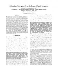
Gain Self-Calibration Procedure for Microphone Arrays Ivan Tashev Microsoft Research, One Microsoft Way, Redmond, WA 98052, USA {
[email protected]} Abstract In many cases microphone arrays, used for beamforming or sound source localization, do not provide the estimated shape of the beam, noise suppression or localization precision. One of the reasons is the difference in the signal paths, caused by different sensitivity of the microphones and/or by the microphone preamplifiers. This paper presents simple and fast procedure for self-calibration of the microphone gains, suitable for real-time applications using microphone arrays for capturing audio signals. It is based on projection of sensor’s coordinates on direction of arrival line and approximation of received energy levels thus reducing the dimensions and speeding up the calculations. The proposed technique automatically calibrates the channels’ gains within ±0.45 dB when the manufacturing tolerance of the microphone sensitivity varies as much as ±4 dB. Tested in real environment.
1. Introduction Algorithms used for processing signals from microphone arrays assume matched channels. Even basic algorithms such as delay-and-sum are quite sensitive to mismatches in the receiving channels, and more sophisticated algorithms for beamforming require very precise matching of the impulse response microphone-preamplifieranalog/digital conversion (ADC) for all channels. The reasons for the channels’ mismatch are mostly manufacturing tolerances of the microphones. Tolerances of the elements in the preamplifiers introduce gain and phase errors as well. In addition, microphone and preamplifier parameters depend on external factors such as temperature, atmospheric pressure, power supply variations, etc. The problem of calibration of microphones and microphone arrays is known and well studied. It can be an expensive and difficult task, particularly for broadband arrays. There are several groups of approaches to calibrate microphones in a microphone array. The calibration can be done for each microphone separately by comparing it with a reference microphone in specialized environment: acoustic tube, standing wave tube, anechoic sound camera
[3]. This approach is very expensive as it requires manual calibration for each microphone and specialized equipment. It is appropriate for calibration of microphones prepared for precise acoustic measurements, but not for general purpose arrays. The next group of calibration methods uses calibration signals (speech, sinusoidal, white noise, acoustic pulses) sent from loudspeaker at known location [4]. In [7] far field white noise is used to calibrate microphone array of two microphones, where the filter parameters are calculated using the NLMS algorithm. Other references suggest using optimization methods to find the microphone array parameters. In [5] the minimization criterion is the speech recognition error. The algorithms in this group require manual calibration after installation of the microphone array and specialized equipment to generate test sounds. The calibration procedure can be combined with calibration of other parts of the whole audio system – acoustic echo cancellation and de-reverberation. Calibration results are used for compensation in real time. They do not reflect changes in the equipment during the exploitation. A separate group of papers cover building algorithms for beamforming and sound source localization that are robust to channels mismatch, i.e. avoiding the calibration at all. Still, theory and practice show that the performance of most of adaptive arrays relies on channel matching. This demands a careful calibration of the array elements to provide good starting point for the adaptation process [5]. The next group of algorithms is self-calibration algorithms. The general approach is described in [1]: find the direction of arrival (DOA) of a sound source assuming that the microphone array parameters are correct, use DOA to estimate the microphone array parameters, and iterate until the estimates converge. Previous discuss estimation of many parameters of the microphone array: sensor positions, gains, and phase shifts. Various techniques are used, from normalized mean-square error minimization to complex matrix methods [2] and high-order statistical parameters estimation [6]. Many of these algorithms are not suitable for practical real-time implementation because of their high CPU load during the normal work of the microphone array.
z
Sound source
Energy
y
Interpolation line
DOA line elevation direction x
d
Microphone array sensors
Figure 1. Sensors projection on DOA line.
Direction of arrival
Figure 2. Received energy interpolation.
2. Channel model and assumptions
3. Self-calibration procedure
To simplify the model of the channel we assume the following: • The microphones in the array have the same shape of their amplitude-frequency characteristics – preferably flat in the work band. This is true with precision better than ±1 dB for the majority of the electret microphones in the band of 100 Hz–8000 Hz. • The microphones have slightly different sensitivity. A typical value here is 55 dB ± 4 dB where 0 dB 1 Pa/V. The assumptions above allow us to simplify significantly the model of the conversion from acoustic signal p(t) to input signal bm(t) for m-th channel: bm (t ) = δ m Gm S m Am p (t − ∆ m ) (1) where δ m is the acoustic decay, Sm is the microphone sensitivity, Am is the preamplifier gain, Gm is the software gain and ∆m is the delay, specific for this channel path. It includes the delay in propagation of the sound wave and the delay in the system microphone-preamplifier. According to [4, pp 158-160] the differences in the phasefrequency characteristics of condenser microphones in the band 200 Hz – 2000 Hz are below 0.25O. The use of low tolerance resistors and capacitors in the preamplifiers (typically 0.1%) provides good matching as well. This simplifies the problem from equalizing the channel’s impulse response to simple gain correction. In addition: a) The sensor positions are known enough precise to ignore the fluency of positions mismatch. b) We have estimator that gives results for horizontal and elevation angles to the sound source (i.e. DOA) when and only when one sound source dominates, i.e. where there is only one sound source and no significant amount of reverberation. c) The sound propagates as a flat wave, i.e. the distance to the sound source is large enough compared to the microphone array size. The goal of the self-calibration procedure is to find set of software gains Gm that provide best channel matching, compensating the differences in the channel parameters.
Consider an array of M microphones with given posir tions vector p . We assume a single sound source at position c = (ϕ ,θ , ρ ) , where ϕ is horizontal angle, θ is elevation angle and ρ is the distance. The sensors sample the signal field at locations pm = ( xm , ym , z m ) : m = 0,1,L , M − 1 . This yields a set of r r signals that we denote by the vector b (t , p ) . The received energy in noiseless and anechoic environment from each sensor is as follows: P 2 Em = ∫ bm (t , pm ) dt ≈ , (2) 2 c − pm
where c − pm
denotes the Euclidian distance between
the sound source and the corresponding sensor, and P is the sound source energy. In case of ambient noise presence, its energy will be added to each channel. For simplicity other factors for energy decay are omitted. The sound source localization provides only the direction of arrival (DOA), i.e. the horizontal angle ϕ and the elevation angle θ . Let’s project the sensor coordinates on the DOA line as shown on Figure 1. This changes the coordinate system from three dimensional to one dimensional. In this coordinate system each sensor has position: (3) d m = ρ m cos(ϕ − ϕ m ) cos(θ − θ m ) , where ( ρ m , ϕ m , θ m ) are the sensor’s coordinates in radial coordinate system: ρ m = xm2 + y m2 + z m2 , ϕ m = arctan xm , ϕ m = arctan xm . y m
y m
Here we assume flat wave due to absence of distance estimation. Figure 2 shows the received energies in the new coordinate system. The new coordinate system allows us to interpolate measured energy levels in each channel with a straight line: ~ E (d ) = a1 d + a 0 , (5)
D iferent distance
Diferent directions 90
60
80 70
40 Energy
30
Error, %
20
50
Energy
40
Error, %
30
10
0 1
0
100 199 298 397 496 595 694 793 892 991 1090
1
Measurement
2 1.8 1.6 1.4 1.2
Gain 2
1
Gain 3
0.8
Gain 4
0.6 0.4 0.2 0 98
265
397
529
661
793
925 1057 1189 1321
Figure 5. Energy and error when distance changes.
4. Implementation
Diferent directions
1
133
M e asure me nt
Figure 3. Energy and error when direction changes.
Channel gains
60
20
10
195 292 389 486 583 680 777 874 971 1068 Measurement
Figure 4. Gains when direction changes.
where a1 and a 0 are such that they satisfy the MMSE requirement: M −1 ~ (6) min ∑ ( E (d i ) − Ei ) 2 . i =0 At this point we have the received energy Em and the ~ estimated energy E (d m ) for each channel. The estimated gain is: E (7) g m = Gmn−1 ~ m , E (d m ) where Gmn−1 is the current gain for this channel. After normalization we receive the final estimated gain: g (8) Gm = m , gA where Gm is the normalized gain and g A is the average of the estimated gains. The final result for sensors gains is G mn = (1 − α )G mn −1 + αG m , (9) where Gmn −1 is the current value of the m-th sensor gain n m
Energy, Error%
Energy, Error%
50
and G is the newly estimated and normalized value. Here α is adaptation parameter.
The self-calibration procedure above was implemented for an eight element equidistant circular microphone array with a diameter of 14 cm and onmidirectional microphones. The microphone array is part of a system for meetings recording and broadcasting, described in [8]. The audio system works with 44.1 kHz sampling rate and 1024 samples per frame, i.e. a frame size of 23.22 ms. Most of known DOA estimation techniques can be used to find the direction to the sound source. The selfcalibration procedure requires receiving DOA estimation only when one sound source (speaker) is dominant. Our implementation uses DOA estimation algorithm, based on beamsteering. The self-calibration procedure is realized as separate processing thread, working in parallel with the main audio stream processing. When a DOA estimate arrives, the procedure calculates the energy of the signal in each channel, projects them on the DOA line and does linear interpolation. After computing the gains, it updates them for using in real-time correction. The necessary measures are taken for stabilization of the calibration process – all intermediate results are verified and in case of improper values the current DOA estimation is rejected. The CPU time cost is only to solve the approximation equation for each DOA estimation that meets the requirements. This happens from 0.5 to 15 times per second, only when someone is talking.
5. Results Several experiments were conducted to verify the selfcalibration algorithm. In a real conference room we recorded all channels gains Gmn (9), the average energy level
σ apr
, where σ apr is the a0 standard deviation of the approximation. All gains equal to one is the starting point for all experiments. The adap-
a0 (5) and the relative error ε =
tive coefficient α is 0.01 for controlled experiments and 0.001 in the real system. The first record contains three segments: silence (i.e. normal room noises), sound source at 90O and sound source at 270O. White noise was used as a sound source (2 sec white noise, 1 sec pause). The chart of average energy and relative error is shown on Figure 3, the channel gains – on Figure 4. For clarity the energy is smoothed with a moving average of five points and only three of eight channel gains are shown. The sound source position doesn’t affect the self-calibration procedure. The gains converge to their values and the relative error goes down smoothly from 29% to 5%. The second record contains data from the same sound source positioned at 0O and distance of 0.65, 1.0 and 1.5 meters. The chart of average energy and relative error is shown on Figure 5. The sound source level is the same, but registered energy decreases with increasing the distance. The gains converge to their values and the relative error goes down smoothly during the first two parts. When the sound source is 1.5 m from the microphone array the relative error goes up to 7% due to worse signal to noise ratio. The noise floor is the same as on figure 3. The worse SNR decreases the precision of the sound source localizer and with increased distance we have more reverberated waves in the input signal. The third group of experiments was recording real meetings with multiple speakers to verify that the gains converge to the same values.
6. Error analysis In the projection of microphone coordinates on the DOA line we assumed sound propagation as flat wave. The relative error in the estimated energy due to flat wave assumption is given by: , (10) 1 ε FW = 1 −
l 1 − m 2d m
where ε FW is the relative error, lm is microphone array size, d m is the distance to the sound source. In our case the microphone array has size of 0.14 meters and the working distance to the speaker is typically from 0.8 to 2.0 meters. The relative error for this distance range is shown in Table 1. We used linear interpolation for process described by a different equation. The average relative error as function of the distance to the speaker is shown in same table as well.
The errors, introduced by the self-calibration method itself, are small. The contribution of other factors (reverberation, signal to noise ratio and DOA estimation error) is much higher. From 5% relative error, to which calibration process converges, only 0.6% is due to the method itself. Very important here is the threshold one/more than one sound sources in the DOA estimator. The adaptive coefficient helps to average the errors and to stabilize the results. Table 1. The relative errors as function of the distance. Distance (m) 0.8 Flat wave error (%) 0.385 Interpolation error (%) 0.252
1.0 0.246 0.161
1.5 0.109 0.071
2.0 0.061 0.040
7. Conclusions The self-calibration procedure described in this paper was deployed on ten meeting capturing stations. For several months of operation it demonstrated stable and reliable work. It removed one step in the station installation – manual calibration of the microphone array. Using the techniques described above, we were able to achieve a channel gain matching within ±0.45 dB, even with microphone elements that have a mismatch of as much as ±4 dB.
8. References [1] H. Van Trees. Detection, Estimation and Modulation Theory, Part IV: Optimum array processing. Wiley, New York. [2] M. Feder and E. Weinstein. “Parameter estimation of superimposed signals system using EM algorithm”. IEEE Trans. Acoustic., Speech and Sig. Proc., vol. ASSP-36, 1988. [3] G.S.K. Wong and T.F.W. Embleton (Eds.), AIP Handbook of Condenser Microphones: Theory, Calibration, and Measurements, American Institute of Physics, New York, 1995. [4] S. Nordholm, I. Claesson, M. Dahl. “Adaptive Microphone Array Employing Calibration Signals. An Analytical Evaluation”. IEEE Trans. on Speech and Audio Processing, December 1996. [5] M. Seltzer, B. Raj. “Calibration of Microphone arrays for improved speech recognition”. Mitsubishi Research Laboratories, TR-2002-43, December 2001. [6] H. Wu, Y. Jia, Z. Bao. “Direction finding and array calibration based on maximal set of nonredundant cumulants”. Proceedings of ICASSP ‘96. [7] H. Teutsch, G. Elko. “An Adaptive Close-Talking Microphone Array”. IEEE Workshop on Applications of Signal Processing to Audio and Acoustics, New York, 2001. [8] R. Cutler, Y. Rui, A. Gupta, JJ Cadiz, I. Tashev, L. He, A. Colburn, Z. Zhang, Z. Liu, S. Silverberg. “Distributed Meetings: A Meeting Capture and Broadcasting System”. Proceedings of ACM Multimedia 2002.