Apr 30, 2017 - SVM's convex formulation and theoretical property [30]. Through comparing length-k local ... arXiv:1704.07468v2 [cs.LG] 30 Apr 2017 ...
GaKCo: a Fast Gapped k-mer string Kernel using Counting Ritambhara Singh, Arshdeep Sekhon, Kamran Kowsari, Jack Lanchantin, Beilun Wang and Yanjun Qi
arXiv:1704.07468v2 [cs.LG] 30 Apr 2017
Department of Computer Science, University of Virginia
Abstract. String Kernel (SK) techniques, especially those using gapped k-mers as features (gk), have obtained great success in classifying sequences like DNA, protein, and text. However, the state-of-the-art gk-SK runs extremely slow when we increase the dictionary size (Σ) or allow more mismatches (M ). This is because current gk-SK uses a trie-based algorithm to calculate cooccurrence of mismatched substrings resulting in a time cost proportional to O(Σ M ). We propose a fast algorithm for calculating Gapped k-mer Kernel using Counting (GaKCo). GaKCo uses associative arrays to calculate the co-occurrence of substrings using cumulative counting. This algorithm is fast, scalable to larger Σ and M , and naturally parallelizable. We provide a rigorous asymptotic analysis that compares GaKCo with the state-of-the-art gk-SK. Theoretically, the time cost of GaKCo is independent of the Σ M term that slows down the trie-based approach. Experimentally, we observe that GaKCo achieves the same accuracy as the state-of-the-art and outperforms its speed by factors of 2, 100, and 4, on classifying sequences of DNA (5 datasets), protein (12 datasets), and character-based English text (2 datasets), respectively 1 . Keywords: Fast Learning, String Kernels, Sequence Classification, Gapped k-mer String Kernel, Counting Statistics
1
Introduction
Sequence classification is one of the most important machine learning tasks used widely in fields like biology and natural language processing. Besides accuracy, one primary requirement for modern sequence classification methods is speed. For example, with the advancement of sequencing technologies, a massive amount of protein and DNA sequence data is produced daily [21]. There is an urgent need to analyze these sequences quickly for assisting time-sensitive experiments. Similarly, on-line information retrieval systems need to classify text sequences, for instance when quickly assessing customer reviews or categorizing documents to different topics. In this paper, we focus on the String Kernels (SK) in the Support Vector Machine (SVM) framework for supervised sequence classification. SK-SVM methods have been successfully used for classifying sequences like DNA [17, 14, 2, 26], protein [12] or character based natural language text [27]. They have provided state-of-the-art classification accuracy and can guarantee nice asymptotic behavior due to SVM’s convex formulation and theoretical property [30]. Through comparing length-k local substrings (k-mers) and incorporating mismatches and gaps, this category of models calculates the similarity (i.e., so-called kernel function) among sequence samples. Then, using such similarity measures, SVM is trained to classify sequences. Recently, Ghandhi et al. [10] developed the state-of-the-art SK-SVM tool called gkm-SVM. gkm-SVM uses a gapped k-mer formulation [11] that reduces the feature space considerably compared to other k-mer based SK approaches. Existing k-mer based SK methods can become very slow or even unfeasible when we increase (1) the number of allowed mismatches (M ) or (2) the size of the dictionary (Σ) (detailed asymptotic analysis in Section 2). Allowing mismatches during substring comparisons is important since most sequences in biology are prone to mutations, i.e., insertions, deletions or substitution of sequence characters. Also, the size of the dictionary varies from one sequence classification domain to another. While DNA sequence is composed of only four characters (Σ = 4), most other domains have bigger dictionary sizes like for proteins, Σ = 20 and for character-based English text, Σ = 36. The state-of-the-art tool, gkm-SVM, may work well for cases with small values of Σ and M (like for DNA sequences with Σ = 4 and M < 4), however, its kernel calculation is slow for cases like DNA with larger M , protein (dictionary size = 20), or character-based English text sequences (dictionary size = 36). Its trie-based implementation, in the worst case, scales exponentially with the dictionary size and the number of mismatches (O(Σ M )). For 1
GaKCo is shared as an open source tool at https://github.com/QData/GaKCo-SVM
5
4 m Ti
e
(G
a
o KC
)=
e
m
Ti
km (g
V -S
1
) M
*
0.9
AUC Score (gkm-SVM)
gkm-SVM Kernel Calculation Time (log seconds)
6
3
2
0.8
0.7
)
C
0.6
1
C AU 0
1
2
3
4
5
0.5
6
GaKCo Kernel Calculation Time (log seconds)
(a)
DNA
(G
Protein
a
o KC
0.6
Text
)=
AU
(g
VM
-S
km
0.7
0.8
0.9
1
AUC Score (GaKCO)
(b)
* Micro-averaged F1-score
Fig. 1. (a) Kernel calculation times (log(seconds)) of GaKCo (X-axis) versus gkm-SVM (Y-axis) for 19 different datasets - protein (12), DNA (5), and text (2). GaKCo is faster than gkm-SVM for 16/19 datasets. (b) Empirical performance for the same 19 datasets (DNA, protein, and text) of GaKCo (X-axis) versus gkm-SVM (Y-axis). GaKCo achieves the same AUC-scores as gkm-SVM.
example, gkm-SVM takes more than 5 hours to calculate the kernel matrix for one protein sequence classification task with only 3312 sequences. This speed limitation hinders the practical applications of SK-SVM. This paper proposes a fast algorithmic strategy, GaKCo: Gapped k-mer Kernel using Counting to speed up the gapped k-mer kernel calculation. GaKCo uses the associative array-based data structure to calculate kernel similarity through cumulative k-mer counting [14]. GaKCo groups the counting of cooccurrence of substrings at each fixed number of mismatches ({0, . . . , M }) into an independent procedure. Such grouping significantly reduces the number of updates on the kernel matrix (an operation that dominates the time cost). This algorithm is naturally parallelizable; therefore we present a multithread variation as our ultimate tool that improves the calculation speed even further. We provide a rigorous theoretical analysis showing that GaKCo has a better asymptotic kernel computation time cost than gkm-SVM. Our empirical experiments, on three different real-world sequence classification domains, validate our theoretical analysis. For example, for the protein classification task mentioned above where gkm-SVM took more than 5 hours, GaKCo takes only 4 minutes. Compared to GaKCo, gkm-SVM slows down considerably especially when M ≥ 4 and for tasks with Σ ≥ 4. Experimentally, GaKCo provides a speedup by factors of 2, 100 and 4 for sequence classification on DNA (5 datasets), protein (12 datasets) and text (2 datasets), respectively, while achieving same accuracy as gkm-SVM. Fig. 1(a) compares the kernel calculation times of GaKCo (X-axis) with gkm-SVM (Y-axis). We plot the kernel calculation times for the best performing (g, k) parameters (see Supplementary Information) for 19 different datasets. We see that GaKCo is faster than gkm-SVM for 16 out of 19 datasets that we have tested. Similarly, we plot the empirical performance (AUC scores or F1-score) of GaKCo (X-axis) versus gkm-SVM (Y-axis) for the best performing (g, k) parameters (see Supplementary) for the 19 different datasets in Fig. 1(b). It shows that the empirical performance of GaKCo is almost the same as gkm-SVM with respect to the AUC scores. In summary, the main contributions of this work are as follows: – Fast: GaKCo is a novel combination of two efficient concepts: (1) reduced gapped k-mer feature space and (2) associative array based counting method, making it faster than the state-of-the-art gapped k-mer string kernel, while achieving same accuracy. – GaKCo can scale up to larger values of m and Σ. – Parallelizable: GaKCo algorithm lends itself to a naturally parallelizable implementation. – We also present a detailed theoretical analysis of the asymptotic time complexity of GaKCo versus state-of-the-art gkm-SVM. This analysis, to our knowledge, has not been reported before. Related Work: Recently, Deep Neural Networks (NNs) have provided state-of-the-art performances for various sequence classification tasks like analyzing DNA [1, 16], proteins [24, 33], and natural language [32, 2
Table 1. List of symbols and their descriptions that are used. Notations D N x, x0 K(x, x0 ) φ(x) l Σ g k M m cgk u η
z Nm (x, x0 ) Cm (x, x0 )
Descriptions Dataset under consideration, D = {x1 , x2 , . . . , xN } Number of sequences in a given dataset D Pair of strings in D that are compared for kernel calculation Kernel Function Feature space of string x Average length of sequences in a given dataset D Size of the dictionary of a given dataset D Length of the gapped instance or g-mer (specified by the user) Length of k-mer inside a gapped instance (specified by the user) Maximum number of allowed mismatches when matching two g-mers. M = (g − k) Number of mismatches between two g-mers. m = {0, . . . M } P =(g−k) g � A notation representing the output of the function M m=0 m Number of unique g-mers in a given dataset D Average size of the nodelist of leafnodes in gkm-SVM’s trie. Each leafnode represents a unique g-mer. Its nodelist includes all g-mers whose hamming distance to the leafnode’s g-mer is up to M Number of unique g-mers with > 1 occurrence in a given dataset D Mismatch profile: number of matching g-mer pairs between x and x0 when allowing m mismatches Cumulative mismatch profile: number of matching {g − m}-mer pairs between x and x0 . Each {g −m}-mer is generated from a g-mer by removing characters from a total of m different positions
28] sequences. Despite their superior performance in accuracy and speed (e.g. through GPUs and minibatches) such NN systems usually require a significant number of training samples. This requirement can be unfeasible for many datasets, especially in the medical research domains. Here, the number of training sequences per experiment can be as low as tens or hundreds due to cost and time constraints. We compare GaKCo’s empirical performance with a state-of-the-art deep convolutional neural network (CNN) model [16]. On datasets with few training samples, GaKCo achieves an average accuracy improvement of 20% over the CNN model (see Fig. 7) making it an appealing tool when the training samples are scarce. Besides, GaKCo includes only two hyperparameters (g and k) for tuning 2 . This feature is desirable when comparing with NN systems for which figuring out the optimal network model and hyperparameters can be a daunting task. The rest of the paper is organized as follows: Section 2 introduces the details of GaKCo and theoretically proves that asymptotically GaKCo runs faster than gkm-SVM for large dictionary or allowing for more mismatches. Section 2.4 discusses the related work. Then Section 3 provides the experimental results we obtain on three major benchmark applications: TFBS binding prediction (DNA), Remote Protein Homology prediction (Proteins) and Text Classification (categorization and sentiment analysis). Empirically, GaKCo shows consistent improvements over gkm-SVM in computation speed across different types of datasets. When allowing a higher number of mismatches, the disparity in speed between GaKCo and the baseline becomes more apparent. Table 1 summarizes the important notations we use.
2
Method
2.1
Background: Gapped k-mer String Kernels
The key idea of string kernels is to apply a function φ(·), which maps strings of arbitrary length into a vectorial feature space of fixed length. In this space, we apply a standard classifier such as Support Vector Machine (SVM) [30]. Kernel-version of SVMs calculates the decision function for an input sample x as: N X f (x) = αi yi K(xi , x) + b (1) i=1
2
There is also one C parameter for tuning SVM training (while using linear kernel)
3
2.5 2 1.5
O
0
ACA CAC
0.5
Spectrum Kernel (g=3,M=0)
O
O O
S = ACACA
Feature Space
1
O
x
x x
x
O
Support Vector Machine
O O
O O
g=3
O
x
x x
x
O
Fig. 2. Overview of the String (Spectrum) Kernel + SVM classifier.
where N is the total number of training samples. String kernels ([17, 14, 10]), implicitly compute K(x, x0 ) as an inner product in the feature space φ(x) as: K(x, x0 ) = hφ(x), φ(x0 )i,
(2)
where x = (s1 , . . . , s|x| ). x, x0 ∈ S. |x| denotes the length of the string x. S represents the set of all strings composed from a dictionary Σ. φ : S → Rp defines the mapping from a sequence x ∈ S to a p-dimensional feature vector. The feature representation φ(·) plays a vital role in string analysis since it is hard to describe strings as feature vectors. One classical method to represent a string is as an unordered set of k-mers, or combinations of k adjacent characters. A feature vector indexed by all k-mers records the number of occurrences of each k-mer in the current string. The string kernel using this representation is called spectrum kernel [18] (see Fig. 2), where the spectrum representation counts the occurrences of each k-mer in a string. Kernel scores between strings are computed by taking an inner product between corresponding “k-mer-indexed” feature vectors: K(x, x0 ) =
X
γ∈Γk
cx (γ) · cx0 (γ)
(3)
where γ represents a k-mer, Γk is the set of all possible k-mers, and cx (γ) is the number of occurrences (with normalization) of k-mer γ in string x. Many variations of spectrum kernels exist in the literature (summarized in Section 2.4) that mostly extend it by including mismatched k-mers when calculating the number of occurrences. Spectrum kernel and its mismatch variations generate extremely sparse feature vectors for even moderately sized values of k, since the size of Γk is Σ k . To solve this issue, Ghandhi et al. [11] introduced a new set of feature representations, called gapped k-mers. It is characterized by two parameters: (1) g, the size of a substring with gaps (we call this gapped instance as g-mer hereafter) and (2) k, the size of non-gapped substring in a g-mer (we call it k-mer). The number of gaps is (g − k). The inner product to compute the gapped k-mer kernel function includes sum over all possible k-mer feature counts obtained from the g-mers: K(x, x0 ) =
X
γ∈Θg
cx (γ) · cx0 (γ)
(4)
where γ represents a k-mer, Θg is the set of all possible gapped k-mers that can appear in all the g-mers (each with (g − k) gaps) in a given dataset (denoted as D hereafter) of sequence samples. The advantage of this formulation is that it reduces the number of possible k-mers drastically. In a “naive” design of gapped k-mer string kernel when selecting k positions (k-mers) from a g-mer, there can � be Σ possible �choices for each of the kg position. Therefore, the total number of possible gapped k-mers equals F = kg Σ k . This feature space grows rapidly with Σ or k. In contrast, Eq. (4) (implemented as gkm-SVM [10]) includes only those k-mers whose gapped formulation has appeared as g-mers in a given dataset D. Θg includes all unique g-mers of the dataset D, whose size |Θg | is normally much smaller than F because the new feature space is restricted to only observable gapped k-mers in D. Ghandhi et al. [10] use this intuition to reformulate Eq.(4) into: 4
0
K(x, x ) =
l1 X l2 X
0
hgk (gix , gjx )
(5)
i=0 j=0
0
For two sequences x and x0 of lengths l1 and l2 respectively. gix and gjx are the ith and j th g-mers of sequences x and x0 (i.e., gix is a continuous substring of x starting from the i-th position and ending 0 at the (i + g − 1)th position of x). hg,k represents the inner product (or similarity) between gix and gjx 0 0 using the co-occurrence of gapped k-mers as features. hgk (gix , gjx ) is non-zero only when gix and gjx have common k-mers. 0
Definition 1. g-pairm (x, x0 ) denotes a pair of g-mers (g1x , g2x ) whose hamming distance is exactly m. 0 g1x is from sequence x and g2x is from sequence x0 . � Each g-pairm (.) has g−m common k-mers, therefore its hgk can be directly calculated as hgk (g-pairm ) = k � g−m . Ghandhi et al. [10] formulate this observation formally into the coefficient hm : k hm =
(
g−m k
0,
�
, if g − m ≥ k otherwise.
(6)
hm describes the co-occurrence count of common k-mers for each possible g-pairm (.) in D. hm > 0 only for cases of m ≤ (g − k) or (g − m) ≥ k. This is because there will be no common k-mers when the number of mismatches (m) between two g-mers is more than (g − k). Now we can reformulate Eq. 5 by grouping g-pairsm (x, x0 ) with respect to different values of m. This is because g-pairsm (.) with same m contribute the same number of co-occurrence counts: hm . Thus, Eq. 5 can be adapted into the following compact form: K(x, x0 ) =
g−k X
Nm (x, x0 )hm
(7)
m=0
Nm (x, x0 ) represents the number of g-pairm (x, x0 ) between sequence x and x0 . Nm (x, x0 ) is named as mismatch profile by [10]. Now, to compute kernel function K(x, x0 ) for gapped k-mer SK, we only need to calculate Nm (x, x0 ) for m ∈ {0, . . . g − k}, since hm can be precomputed. The state-of-the-art tool gkm-SVM [10] calculates Nm (x, x0 ) using a trie based data structure that is similar to [17] (with some modifications, details in Section 2.3). 2.2
Proposed Method: Gapped k-mer Kernel with Counting (GaKCo)
In this paper, we propose GaKCo, a fast and novel algorithm for calculating gapped k-mer string kernel. GaKCo provides superior time performance over the state-of-the-art gkm-SVM and is different from it in three aspects: – Data Structure. gkm-SVM uses a trie based data structure (plus a separate nodelist at each leafnode) for calculating Nm (see Figure 3(c)). In contrast, GaKCo uses simple associative arrays. – Algorithm. GaKCo performs g-mer based cumulative counting of co-occurrence to calculate Nm . – Parallelization. GaKCo groups computations for each value of m into an independent function, making it naturally parallelizable. We, therefore, provide a parallel version that uses multi-thread implementation. Intuition : When calculating Nm between all pairs of sequences in D for each value of m (m ∈ {0, . . . , M = g − k}), we can use counting to process all g-pairsm (.) (details below) from D together. Then we can calculate Nm from such count statistics of g-pairsm (.). This method is entirely different from gkm-SVM that uses a trie to organize g-mers such that each leafnode’s (a unique g-mer’s) nodelist memorizes its mismatched g-mer neighbors in D for up to g − k mismatches. Section 2.3 provides theoretical analysis that GaKCo formulation is asymptotically more scalable to M and Σ than gkm-SVM. 5
(a)
S=ACACA T=AAACA g-mers ACA CAC ACA AAA AAC ACA m=1 Step4
g-mers Index ACA S CAC S ACA S AAA T AAC T ACA T
m=0 Step1 Step3 j=1 ACA CAC ACA AAA AAC ACA
Array AA T AC S AC T CA S CA S CA T
S S S T T T
position 1 Step5
Step6
Array AAA AAC ACA ACA ACA CAC j=1
ACA S CAC S ACA S AAA T AAC T ACA T position 2
S T S 0 2 Nm=0 = T 2 0
()
3 -1
(b) Step1
Count Operation
m=0
Kernel Update
AAA ACA ACA ACA
Matching g-mers Removing symbols from position i (=m)
Array AA AA AA AA AC CC
+
0 (2+1) = 0 3 3 0 (2+1) 0 0 9 Nm=1 = 9 0 C1
T T S S T S
Sort Operation
Step2
0 4 4 0 0 2 2 0 Nm=0
j=1 S S T T T S
ACA S CAC S ACA S AAA T AAC T ACA T position 3
+
Array AA T AA T AC S AC S AC T CA S 0 2 2 0
S T = S 0 3 T 3 0 Nm=1
Step3 & Step4 m=1 AAA T ACA S ACA S ACA T 1+1=2
T S S T
Step2 Nm=0(S,T)= 1+1 =2 Step6
ACA T ACA S AAA S AAA T 2+2=4
AA T ACA S ACA S ACA T 1+1=2
Step5 Cm=1 (S,T)= 2+4+2=8
Nm=1 (S,T)= 2 (from direct observation) 3 Cm=1(S,T)= Nm=1(S,T) + 1 Nm=0(S,T) Cm=1 (S,T)= 2 + 3x2 = 8
=
S T S 0 9 T 9 0
(c) A A
C1 A (T)
Sequence list (ACA) S T
C A (S,T)
Leaf Node
()
m=0 m=1
Nodelist (ACA) S/ACA T/ACA T/AAA
Fig. 3. Overview of GaKCo algorithm for calculating mismatch profile Nm (S, T ). Given two strings S = ACACA and T = AAACA, and g = 3, we can get g-mers {ACA, CAC, ACA} and {AAA, AAC, ACA} respectively. [Step 1] For m = 0, all the g-mers are sorted lexicographically. [Step 2] Nm=0 (S, T ) is calculated directly by using sorting and counting to get the counts of matching g-mer ACA in each string (S/2, T /1). Then the kernel update operation updates Nm=0 (S, T ) value to� 2. [Step 3] For m = 1, we perform over counting of the g − 1-mers by picking 1 position at a time (from g=3 positions) and removing symbols from each of these positions to obtain 1 (g − 1)-mers. [Step 4] We sort and count to find the number of matching (g − 1)-mers for each picked position. � [Step 5] Summing up over all g=3 positions, we get cumulative mismatch profile Cm=1 . Cm=1 includes matching 1 statistics of g-mers with both mismatches m = 1 and m = 0. [Step 6] Using Eq. 9 we get Nm=1 (S, T ) = 3 from Cm=1 (S, T ) = 9 and Nm=0 (S, T ) = 2. This count corresponds exactly to the actual number of pairs of g-mers at hamming distance m = 1 between s and t (i.e. {ACA : s/2, AAA : t/1}, {CAC : s/1, AAC : t/1}). [Note: we do not calculate Nm (.) between a string and itself, i.e Nm (S, S) or Nm (T, T )] (b) A case demonstration of the overcounting that takes place when calculating Cm=1 . (c) A case demonstration of two leafnode g-mers and associated nodelist for leaf {ACA} in the trie used by gkm-SVM.
Algorithm: GaKCo calculates Nm (x, x0 ) as follows (for pseudo code, see Algorithm 1): 1. GaKCo first extracts all possible g-mers from all the sequences in D and puts them in a simple array. Given that there are N number of sequences with average length l 3 , the total number of g-mers is N × (l − g + 1) ∼ N l (see Fig. 3 (a)).
2. Nm=0 (x, x0 ) represents the number of g-pairm=0 (x, x0 ) (pairs of g-mers whose hamming distance is 0) between x and x0 . To compute Nm=0 (xi , xj ) ∀i, ∀j = 1, ..., N , GaKCo sorts all the g-mers lexicographically (see Fig. 3(a) [Step 1]) and counts the occurrences (if > 1) of each unique g-mer. Then we use these counts and the associated indexes of sequences to update all the kernel entries for sequences that include the matching g-mers (Fig. 3(a) [Step 2]). This computation is straight-forward and the sort and count step takes O(gN l) time cost while the kernel update costs O(zN 2 ) (at the worst case). Here, z is the number of g-mers that occur > 1 times. 3. For cases when m = 1, . . . (g − k), we use a statistics measure Cm (x, x0 ), called cumulative mismatch profile between two sequences x and x0 . This measure describes the number of matching (g −m)-mers between x and x0 . Each (g − m)-mer is generated from a g-mer by removing a total number of m positions. We can calculate the exact mismatch profile Nm from the cumulative mismatch profile Cm for m > 0 (explanation in the next step). 3
This is a simplification of real world datasets in which sequence length varies across samples
6
Cm=1 can be calculated from the associative-array (containing all g-mers in D and their counting statistic) that we obtain from calculating Nm=0 . When m = 1, we perform the following operation on the list of all g-mers: we first pick 1 position and remove the symbol from the same position for all g-mers to get a new list of (g − 1)-mers (Fig. 3 (a) [Step 3]). We then sort and count this new list to get the number of matching (g − 1)-mers (Fig. 3 (b) [Step 4]). For the sequences that have the matching (g − 1)-mers, we add the counts into �their corresponding entries in matrix Cm . This sequence of operations is repeated for a total of g1 positions, i.e every position that can be removed from g-mers to �get (g − 1)-mers. The cumulative mismatch profile Cm=1 is equal to the sum of all counts from all g1 runs (Fig. 3 [Step 5]). We use the same procedure for calculating Cm for m = 2, ..., M = g − k.
4. We now calculate Nm from Cm and Nj for j = 0, ..., m − 1. First, we explain the relationship between Cm and Nm . Given two g-mers g1 and g2 , we remove symbols from the same set of m positions of both g-mers to get two (g − m)-mers: g10 and g20 . If the hamming distance between g10 and g20 : d(g10 , g20 ) = 0, then we can conclude that the hamming distance between the original two g-mers g1 and g2 : d(g1 , g2 ) ≤ m (See formal proof in Supplementary). For instance, Cm=1 (x,x’) records the statistic of matching (g − 1)-mers among x and x0 . It not only includes the matching statistics of all g-mer pairs whose hamming distance is m = 1, but it also over-counts the matching statistics of all g-mer pairs whose hamming distance is m = 0. This is because the matching g-mers that were counted for m = 0� will also contribute to the matching statistics when considering (g − 1)-mers and that too for g1 times! Similarly, this over-counting occurs for other values of m as well. Essentially the cumulative mismatch profile Cm can be formulated as: ∀m ∈ {0, . . . , g − k} C m = Nm +
m−1 X� j=0
� g−j Nj m−j
(8)
We demonstrate this over-counting using Fig. 3(b) on a subset of g-mers (ACA,AAA) from Fig. 3(a). Using Eq.8, the exact mismatch profile Nm can be computed as follows: Nm = C m −
m−1 X� j=0
� g−j Nj m−j
(9)
Here, we subtract Nj (for j = 0, . . . , i − 1) from Cm to compensate for the over-counting described above. Parallelization: For each value of m from {0, . . . M = g − k}, calculating Cm is independent from other values of m. Therefore, GaKCo’s algorithm can be easily revised into a parallel version. Essentially, we just need to revise Step 9 in Algorithm 1 (pseudo code) - “For each value of m”- into, “For each value of m per machine/per core/per thread”. In our current implementation, we create a thread for each value of m from {0, . . . M = g − k} and calculate Cm in parallel. In the end, we compute the final kernel matrix K using all the resulting Cm matrices. Fig. 5 and 7(b) show the improvement of kernel calculation speed when comparing the multi-thread version with the single-thread implementation of GaKCo. 2.3
Theoretical Comparison of Time Complexity
In this section we conduct asymptotic analysis to compare the time complexities of GaKCo with the state-of-the-art toolbox gkm-SVM. Time Complexity of GaKCo: The time cost of GaKCo splits into two groups: (1) Pre-processing: those operations that indirectly update the matching statistics among sequences; (2) Kernel updates: those operations that directly update the matching statistics among sequences. Pre-processing: For each possible m (m ∈ {0, . . . M = g − k}), GaKCo needs to choose m positions for symbol removing (Fig. 3 (a) [Step 3]), and then sort and count the possible (g − m)-mers from D (Fig. 3 7
Implementations GaKCo gkm-SVM [10] Pre-processing cgk gN l ug Kernel updates cgk zN 2 ηuN 2
Table 2. Comparing time complexity. gvm-SVM’s time cost is O(ug + ηuN 2 ). GaKCo’s time complexity is O(cgk [gN l + zN 2 ]). In gkm-SVM the term ηuN 2 dominates the time. For GaKCo the term cgk zN 2 dominates the time cost.
� M =g−k g � g M (a) [Step 4]). Therefore the time cost of pre-processing is O(Σm=0 (g − m)N l) ∼ O(Σm=0 gN l). m m PM =(g−k) g � To simplifying notations, we use cgk to represent m=0 m hereafter. Kernel Updates: These operations update the entries of Cm or Nm matrices when GaKCo finishes each round of counting the number of matching (g − m)-mers. Assuming z denotes the number of unique (g − m)-mers that occur � >2 1 times, the 2time cost of kernel update operations is (at the worst g M case) equivalent to O(Σm=0 m zN ) ∼ O(cgk zN ). Therefore, the overall time complexity of GaKCo is O(Cgk [gN l + zN 2 ]). gkm-SVM Algorithm Now we introduce the algorithm of gkm-SVM briefly. Given that there are N sequences in a dataset D, gkm-SVM first constructs a trie tree recording all the unique g-mers in D. Each leafnode in the trie stores a unique g-mer (more precisely by its path to the rootnode) of D. We use u to denote the total number of the unique g-mers in this trie. Next, gkm-SVM traverses the tree using the order of depth-first. For each leafnode (like ACA in (Fig. 3 (c)), it maintains a nodelist that includes all those g-mers in D whose hamming distance to the leafnode g-mer ≤ M . When accessing a leafnode, all mismatch profile matrices Nm (x, x0 ) for m ∈ {0, . . . , M = (g − k)} are updated for all possible pairs of sequences x and x0 . Here x consists of the g-mer of the current leafnode (like S/ACA in (Fig. 3 (c)). x0 belongs to the nodelist’s sequence list. x0 includes a g-mer whose hamming distance from the leafnode is m (like T /ACA(m = 0) or T /AAA(m = 1) in (Fig. 3 (c)). Time Complexity of gkm-SVM: We also split operations of gkm-SVM into those indirectly (preprocessing) or directly (kernel-update) updating Nm . Pre-processing: Assuming u unique g-mers exist in D, then the number of leafnodes in the trie is u. The time taken to construct the trie equals O(ug). Kernel Update: For each leafnode of the trie (total u nodes), for each g-mer in its nodelist (assuming average size of nodelist is η), gkm-SVM uses the matching count among g-mers to update involved sequences’ entries in Nm (if hamming distance between two g-mers is m). Therefore the time cost is O(ηuN 2 ) (at the worst case). Essentially η represents on average the number of unique g-mers (in the trie) that are at a hamming distance up to M from the current leafnode. That is η = min(u,
M =(g−k) �
X
m=0
� g (Σ − 1)m ) ∼ min(u, cgk (Σ − 1)M ) m
(10)
Fig. 4 shows that η grows exponentially to M until reaching its maximum u. The total complexity of time cost from gkm-SVM is thus O(ug + uηN 2 ). Asymptotically, at the worst case when η = u, the time complexity of gkm-SVM is O(ug + u2 N 2 ). Comparing Time Complexity of GaKCo with gkm-SVM: Table 2 compares the asymptotic time cost of GaKCo with gkm-SVM. Asymptotically the time complexity of gvm-SVM is O(ug + ηuN 2 ). For GaKCo the overall time complexity is O(cgk [gN l + zN 2 ]). In gkm-SVM the term O(ηuN 2 ) dominates the overall time. For GaKCo the term O(cgk zN 2 ) dominates the time cost. For simplicity, we assume that z = u even though z ≤ u. Upon comparing O(η × uN 2 ) of gkm-SVM with O(cgk × uN 2 ) of GaKCo, clearly the difference lies between the terms η in gkm-SVM and cgk in GaKCo. In details, – η ∼ cgk (Σ − 1)M (gkm-SVM) versus cgk (GaKCo): For a given g-mer � g, the number of possible g g-mers that are at a distance M from it is cgk (Σ − 1)M . That is, M positions can be substituted with (Σ − 1)M possible characters. Thus in gkm-SVM, the estimated size η grows exponentially with number of allowed mismatches M . We show the trend of function f = cgk (Σ − 1)M in Fig. 4 (a) for three different domains - TF-DNA (Σ = 4), SCOP-protein (Σ = 20) and text (Σ = 36) by varying the values of M for g = 10. We threshold these curves at u = 6 × 10⁴ , which is the average observed 8
value of u across multiple datasets. In Fig. 4 (a), when dictionary size Σ is small (=4), the size of the nodelist η is mostly smaller than u. But when Σ is larger than 4, η gets larger than u for M ≥ 4. In contrast, GaKCo’s term cgk is independent of the dictionary size Σ. – η = u (gkm-SVM) versus cgk (GaKCo): For large dictionary size (e.g. Σ = 20), size of the nodelist η mostly equals to u in gkm-SVM. Even for cases with small dictionary size (e.g. Σ = 4) η is close to u for M ≥ 4. While gkm-SVM might be fast for small Σ and M < 4, its kernel calculation time will slow down considerably for M ≥ 4. For example, for one of the SCOP datasets, when g = 10, count of unique g-mers u = 6 × 10⁴ at M = 4 (close to u shown in Fig. 4 (a)). Therefore, at a modest value of M = 4 η = 6 × 10⁶ for gkm-SVM while cgk = 210 for GaKCo. The former is approximately 300 times higher than GaKCo.
12
Algorithm 1 GaKCo
11 10
log (
)
9 8 7
u ~600,000
6 5 4 3 2 1
1
2 DNA( =4)
3
5 4 M=(g-k) Protein( =20)
6
7
Text ( =36)
Fig. 4. η: estimated size of nodelist used in gkm-SVM [10]. It is equal to the number of g-mers with M mismatches from the current g-mer at the trie-leafnode. For a given g-mer g, the number of possible g-mers that are at a distance M is roughly cgk (Σ − 1)M . The size grows exponentially with the number of mismatches m. When dictionary size Σ is small, η < u. However when Σ > 4 and m ≥ 4, η ≤ u.
2.4
Require: L, g, k . L=Array list of g-mers 1: procedure CalculateKernel(L,g,k) 2: M ←g−k 3: N←MismatchProfile(L,g,M ) 4: K←0 5: for m : 0 → M �do 6: hm ← g−M k 7: K ← K + Nm .hm 8: procedure MismatchProfile(L,g,M ) 9: for m : 0 → M do . Parallel threads 10: Cm ← 0 � . Cumulative Profile g 11: npos ← m . Number of positions 12: for i : 0 → npos do i 13: Cm ←0 i 14: L ← removeP osition(L, i) 15: Li ← sort(Li ) i 16: Cm ← countAndU pdate(Li ) i 17: Cm ← Cm + Cm 18: for m : 0 → M do 19: for j : 0 → m − 1 do � g−j 20: Nm ← Cm − m−j Nm return N . N ∈ {N0 , . . . , NM } Ensure: K . Kernel Matrix
Connecting to Previous Studies
String Kernels Aside from the spectrum kernel [17] and gapped k-mer kernel [10], a few other notable string kernels include (but are not limited to): (1) (k, m)-Mismatch Kernel. This kernel calculates the dot product of contiguous k-mer counts with m mismatches allowed. The cumulative matching statistic idea was first proposed by [14] for this kernel. 4 (2) Substring Kernel. It measures the similarity between sequences based on common co-occurrence of exact matching subpatterns (e.g., substrings) [31]. (3) Profile Kernel. This method uses the notion of similarity based on a probabilistic model (e.g. profile) [13]. (4) Cluster Kernel. The “sequence neighborhood” kernel or “cluster” kernel [7] is a semi-supervised extension of the string kernel. It replaces every sequence with a set of “similar” (neighboring) sequences and obtains a new representation. Then, it averages over the representations of these contiguous sequences found in the unlabeled data using a sequence similarity measure. k-mer counting methods k-mer (or in our case, g-mer) counting is the method by which we determine the number of matching or unique k-mers (or g-mers) in any text or pattern. Tools handling large text datasets need to filter out these unique k-mers (or g-mers) to reduce the processing or counting time. GaKCo uses a ‘sort and count’ method for calculating the number of matching g-mers to compute 4
Because [14] uses all possible k-mers built from the dictionary with m mismatches as the feature space, the authors [14] need to precompute a complex weight matrix to incorporate all possible k-mers with m mismatches.
9
Table 3. Details of datasets used for different prediction tasks. All tasks, except WebKB, are binary classification tasks. WebKB is a multi-class classification dataset with four classes: project, course, faculty, and student. Training Testing Sample properties Prediction Task Repo Datasets Pos seq Neg seq Pos seq Neg seq N Σ Max(l) CTCF EP300 TF Binding Site ENCODE JUND 1000 1000 1000 1000 4000 5 100 (DNA) RAD21 SIN3A 1.1 1150 1189 8 1227 3574 1.34 866 1209 6 1231 3312 Remote Protein Homology SCOP 2.19 110 1235 9 1206 2560 20 905 (Protein) 2.31 1063 1235 8 1194 3500 2.1 4763 1229 120 950 7062 2.34 286 1215 6 1231 2738 2.41 192 1235 6 1213 2646 2.8 56 1185 8 1231 2480 3.19 922 1181 7 1231 3341 3.25 1187 1208 11 1231 3637 3.33 466 1214 7 1231 2918 3.50 105 1231 8 1205 2549 Stanford Treebank Sentiment 3883 3579 877 878 9217 36 260 Text Classification Dataset from [5] WebKB 335, 620, 744, 1083 166, 306, 371, 538 4163 36 14218
the mismatch profile (Section 2.2). This is a widely used method that lists all the g-mers, sorts them lexicographically and counts all the consecutive matching entries while skipping the unique g-mers. It has been used previously in tools used for genome assembly [22], discovery of motifs (or most common fixed length patterns) [25], and string kernel calculation [14]. BioSequence Classification with Deep Learning In recent years, deep learning models have become popular in the bioinformatics community, owing to their ability to extract meaningful representations from large labeled datasets (e.g., with sample size ∼30,000 sequences). For example, Qi et al. [24] used a deep multi-layer perceptron (MLP) architecture with multitask learning to perform sequence-based protein structure prediction. Zhou et al. [33] created a generative stochastic network to predict secondary structure on the same data as used by Qi et al. [24]. Recently, Lin et al. [19] outperformed all the state-of-the-art works for protein property prediction task by using a deep convolutional neural network architecture. Later, Alipanahi et al. [1] applied a convolutional neural network model for predicting sequence specificity of DNA and RNA-binding proteins as well as generating motifs, or consensus patterns, from the features that were learned by their model. Lanchantin et al. [16] proposed a deep convolutional/highway MLP framework for the same task and demonstrated improved performance. In the field of natural language processing, multiple works like [29] have used deep learning models for document [32] or sentiment [28] classification.
3 3.1
Experiments Benchmark Tasks of Sequence Classification
DNA and Protein Sequence Classification Studying DNA and Protein sequences gives us deeper insight into the biological processes that can, in turn, help us understand cell development and diseases. Two major tasks essential in the field are Transcription Factor Binding Site (TFBS) Prediction and Remote Protein Homology Prediction. Transcription factors (TFs) are regulatory proteins that bind to functional sites of DNA to control the regulation of genes. Each different TF binds to specific locations (or sites) on a genomic sequence to regulate cell machinery. Owing to the development of chromatin immunoprecipitation and massively parallel DNA sequencing (ChIP-seq) technologies [23], maps of genome-wide binding sites are currently available for multiple TFs across different organisms. Because ChIP-seq experiments are slow and expensive, computational methods to identify TFBSs accurately are essential for understanding cell regulation. 10
Remote Protein Homology Prediction, i.e. classification of protein sequences according to their biological function or structure, plays a significant role in drug development. Protein sequences that are a part of the same protein superfamily are evolutionally related and functionally and structurally relevant to each other [3]. Protein sequences with feature patterns showing high homology are classified into the same superfamily. Once assigned a family, the properties of the protein can be easily narrowed down by analyzing only the superfamily to which it belongs. Researchers have formulated both these tasks as classification tasks, where knowing a DNA or protein sequence, we would like to classify it as a binding site or non-binding site for TF prediction and belonging or not belonging to a protein family for homology prediction respectively. Text Classification Text classification incorporates multiple tasks like assigning subject categories or topics to documents, spam detection, language detection, sentiment analysis, etc. Generally, given a document and a fixed number of classes, the classification model has to predict the class that is most relevant to that document. Several recent studies have discovered that character-based representation provides straightforward and powerful models for relation extraction [27], sentiment classification [32], and transition based parsing [4]. Lodhi et. al. [20] first used string kernels with character level features for text categorization. However, their kernel computation used dynamic programming which was computationally intensive. Over recent years, more efficient string kernel methods have been devised [17, 13–15, 10]. Therefore, we use simple character-based text input for document and sentiment classification task. We perform 19 different classification tasks to evaluate the performance of GaKCo. These tasks belong to the discussed three categories: (1) TF binding site prediction (DNA dataset), (2) Remote Protein Homology prediction (protein dataset), and (3) Character-based English text classification (text dataset). 3.2
Experimental Setup
Datasets: ENCODE ChIP-Seq DNA Sequences: Maps of genome-wide binding sites are currently available for multiple TFs for human genome via the ENCODE [8] database. These ChIP-seq “maps” mark the positions of the TF binding sites. We select 100 basepair sequences overlapping the binding sites as positive sequences and randomly select non-binding sequences from the human genome as negative sequences. We perform this selection for five different transcription factors (CTCF, EP300, JUND, RAD21, and SIN3A) from the K562 (leukemia) cell type, resulting in five different prediction tasks. We select 2000 sequences for training that consist of 1000 positive and negative samples each. For testing, we use another set of 2000 sequences with 1000 positive and negative samples each. We use the dictionary size of 5 (Σ = 5). There are four nucleotide symbols - A, T, C, G - in the DNA. Additionally, sometimes sequences have ‘N’ for nucleotides that are not read by the sequencing machines. Therefore, the dictionary is {A,T,C,G,N}. SCOP Protein Sequences: The SCOP domain database consists of protein domains, no two of which have 90% or more residual identity [12]. It is hierarchically divided into folds, superfamilies, and finally families. We use 12 sets of samples (listed in Table 3.1) and select positive test sequences (for each sample) from 1 protein family of a particular superfamily. We obtain the positive training sequences from remaining families in that superfamily. We select negative training and test sequences from non-overlapping folds outside the positive sequence fold. We use the dictionary size of 20 (Σ = 20) as there are 20 amino acid symbols that make up a protein sequence. Therefore the dictionary is {A,C,D,E,F,G,H,I,K,L,M,N,P,Q,R,S,T,V,W,Y}. WebKB and Sentiment Classification Datasets: The documents in the WebKB are web pages collected by the World Wide Knowledge Base project of the CMU text learning group and were downloaded from The 4 Universities Data Set Homepage. These pages were collected from computer science departments of various universities in 1997. We downloaded the processed datasets (removed stop/short words, stemming, etc.) from [5]. This task is a multi-class classification task with four classes: project, course, faculty, and student. For the sentiment analysis experiments, we used the Stanford sentiment treebank dataset [28]. This dataset provides a score for each sentence between 0 and 1 with [0, 0.4] being negative sentiment and [0.6, 1.0] being positive. We combined the validation set in the original treebank dataset with the training set. We use the dictionary size of 36 (Σ = 36) since we use character-based input. The dictionary includes all the alphabets [A-Z] and numbers [0-9]. Details of the datasets are in Table 3. 11
3 2.5 2 1.5 1
1
2
3
4
5 6 M = (g - k)
7
8
9
5 4.5 4 3.5 3 2.5 2 1.5 1 0.5
1
(a) DNA (EP300)
2
3
4
5 6 M = (g-k)
7
8
9
Kernel Calculation Time (log seconds)
4 3.5
Kernel Calculation Time (log seconds)
Kernel Calculation Time (log seconds)
4.5
5 4.5 4 3.5 3 2.5 2 1.5
1
GaKCo (Single thread)
3
4 5 M = (g- k)
6
7
(c) Text (Sentiment)
(b) Protein (1.34) GaKCo
2
gkm-SVM
Fig. 5. Kernel calculation times (lower is better) for best g and varying k with M = (g − k) = {1, 2, . . . g − 1} hyperparameters for (a) EP300 (DNA,Σ = 5), (b) 1.34 (protein, Σ = 20), and (c) Sentiment (text, Σ = 36) datasets. The best performing hyperparameters (g, k or M = (g − k)) are highlighted as red colored dashed lines. For GaKCo, results are shown for both single thread and multi-thread implementations. GaKCo (single thread) outperforms gkm-SVM for a large dictionary size (Σ > 5) and a large number of mismatches M ≥ 4, confirming our analysis in Section 2. The final GaKCo (multi-thread) implementation further improves the performance. For protein dataset (b) gkm-SVM takes > 5 hours to calculate the kernel, while GaKCo calculates it in 4 minutes.
Baselines: We compare the kernel calculation times and empirical performance of GaKCo with gkm-SVM [10]. We also run the CNN implementation from [16] for all the datasets. Classification: After calculation, we input the N × N kernel matrix into an SVM classifier as an empirical feature map using a linear kernel in LIBLINEAR [9]. Here N is the number of sequences in each dataset. The SVM maximizes the margin between the positive and negative instances of the samples in the kernel defined feature space. For the multi-class classification of WebKB data, we use the multi-class version of LIBSVM [6]. Model parameters: We vary the hyperparameters g ∈ {7, 8, 9, 10} and k ∈ {1, 2, . . . , g − 1} of both GaKCo and gkm-SVM. M = (g − k) for all these cases. We also tune the hyperparameter C ∈ {0.01, 0.1, 1, 10, 100, 1000} for the SVM. We present the results for the best g, k, and C values based on the empirical performance metric. We ran the CNN model with default parameters for 50 epochs (number of training and testing times), and we present the results for the epoch with the best empirical performance metric. Evaluation Metrics: Running time: We compare the kernel calculation times of GaKCo and gkm-SVM in seconds. In some figures, we have represented time in log-scale (log(seconds)) to accommodate large values. All runtime experiments have been performed on AMD Opteron(TM) Processor 6376 @ 2.30GHz with 250GB memory. Empirical performance: We use the Area Under Curve (AUC) score (from the Receiver Operating Characteristic (ROC) curve) as our empirical evaluation metric for 18 binary classification tasks. We report the results of WebKB multi-class classification using micro-averaged F1 score. 3.3
Kernel Calculation Time Performance
Our experimental results confirm our theoretical analysis in Section 2 that GaKCo has a lower kernel calculation time than gkm-SVM. Fig. 1(a) shows GaKCo is faster than gkm-SVM for 16/19 tasks. The other three tasks for which GaKCo records similar kernel calculation times are DNA sequence prediction tasks. This is expected as DNA has a smaller dictionary size (Σ = 5) and thus, for a small number of allowed mismatches (M ) gkm-SVM gives comparable speed performance. We elaborate on this further in the following discussion. GaKCo scales better than gkm-SVM for large dictionary size (Σ) and large number of mismatches (M ): Fig. 5 shows the kernel calculation times of GaKCo and gkm-SVM for the best-performing g and varying 12
1000
3
2.5 2
1.5 =5 (DNA)
=20 (Protein)
Dictionary Size ( ) GaKCo
(a)
gkm-SVM
=36 (Text)
800
2
1.5
600 400
1
0.5
200 0
3
2.5
1200
3.5
Kernel calculation time (log(seconds))
1400
4
1
3.5
1600
Average kernel calculation time (seconds)
Average kernel calculation time (log (seconds))
5
4.5
=5 (DNA)
=20 (Protein)
=36 (Text)
Dictionary Size ( ) GaKCo (Multithread)
(b)
GaKCo (Single Thread)
0
DNA
(EP300)
Protein
Text
DNA
(1.34) (Sentiment) (EP300)
GaKco
N=100
Protein
Text
(1.34) (Sentiment)
gkm-SVM
N=250
N=500
N=750
(c)
Fig. 6. (a) Average kernel calculation times (lower is better) for the best performing (g, k) parameters for DNA (Σ = 5), protein (Σ = 20), and text (Σ = 36) datasets. gkm-SVM takes similar time as GaKCo to calculate the kernel for DNA dataset but slows down considerably for protein and text datasets due to increase in dictionary size. Since GaKCo is independent of the dictionary size, it is consistently faster for all three datasets. (b) Average kernel calculation times (lower is better) across DNA (5), protein (12) and text (2) datasets. Multi-thread GaKCo implementation improves the kernel calculation speed of the single-thread GaKCo by a factor of 2. (c) Kernel calculation times (lower is better) of GaKCo and gkm-SVM for best performing parameters (g, k) for: EP300 (DNA), 1.34 (protein), and Sentiment (text) datasets. Length of the sequences for all three datasets is fixed to l = 100 and number of sequences are varied for N = {100, 250, 500, 750}. With increasing number of sequences, the increase in kernel calculation time is more drastic for gkm-SVM than for GaKCo across all three datasets.
k = {1, 2, . . . (g − 1)} for three binary classification datasets: (a) EP300 (DNA), (b) 1.34 (protein), and (c)Sentiment (text) respectively. We select these three datasets as they achieve the best AUC scores out of all 19 tasks (see Supplementary). We fix g and vary k to show time performance for different number of allowed mismatches i.e. M = (g − k) = {1, 2, . . . (g − 1)}. For GaKCo, the results are plotted for both single-thread and the multi-thread implementations. We refer to the multi-thread implementation as GaKCo because that is our final code version. Our results show that GaKCo (single-thread) scales better than gkm-SVM for a large dictionary size (Σ) and a large number of mismatches (M ). The final version of GaKCo (multi-thread) further improves the performance. Details for each dataset are as follows: – DNA dataset (Σ = 5): In Fig. 5 (a), we plot the kernel calculation times for best g = 10 and varying k with M = {1, 2, . . . 9} for EP300 dataset. As expected, since the dictionary size of DNA dataset (Σ) is small, gkm-SVM performs fast kernel calculations for M = (g − k) < 4. However, for large M ≥ 4, its kernel calculation time increases considerably compared to GaKCo. This result connects to Fig. 4 in Section 2, where our analysis showed that the nodelist size becomes closer to u as M increases, thus increasing the time cost. – Protein dataset (Σ = 20): Fig. 5 (b), shows the kernel calculation times for best g = 10 and varying k with M = (g − k) = {1, 2, . . . 9} for 1.34 dataset. Since the dictionary size of protein dataset (Σ) is larger than DNA, gkm-SVM’s kernel calculation time is worse than GaKCo even for smaller values of M < 4. This also connects to Fig. 4 where the size of nodelist ∼ u even for small M for protein dataset, resulting in higher time cost. For best-performing parameters g = 10, k = 1(M = 9), gkm-SVM takes 5 hours to calculate the kernel, while GaKCo calculates it in 4 minutes. – Text dataset (Σ = 36): Fig. 5 (c), shows the kernel calculation times for best g = 8 and varying k with M = {1, 2, . . . 7} for Sentiment dataset. The results follow the same trend as presented above. For large M ≥ 4, kernel calculation time of gkm-SVM is slower as compared to GaKCo. One would expect that with large dictionary size (Σ) the performance difference will be same as that for protein dataset. However, unlike protein sequences, where the substitution of all 20 characters in a g-mer is equally likely, text dataset has an underlying structure. Concretely, the chance of substitution of some characters in a g-mer will be higher than others. For example, in a given g-mer “my nam”, the last position is more likely to be occupied by ‘e’ than ‘z’. Therefore, even though the dictionary size is large, the growth of the nodelist is restricted by the underlying structure of the text. Therefore, while GaKCo’s time performance is consistent across all three datasets, gkm-SVM’s time performance varies due to the characteristic properties (like dictionary size (Σ)) of the datasets. 13
(b)
4 3.5
0.4 0.3
2
0.2
1.5 1
0.1
0.5 0
1 2 3 4 5 6 Kernel Calculation Time (log(seconds))
Text (GaKCo) DNA (GaKCo) Protein (GaKCo) DNA (gkm-SVM) Protein (gkm-SVM) Text(gkm-SVM)
0
19 String Classification Tasks DNA
0.80
0.85
AUC Score
AUC Score
0.80 0.75 0.70 0.65
*
-0.1
250
500
Training Set Size DNA (SIN3A)
750
* Micro-averaged F1-score
0.8
0.70
0.7
0.60
0.40
Text
0.9
0.6
0.50 100
Protein
Micro F1-Score
Memory used (GB)
3 2.5
(c)
0.5
Difference between AUC Scores (GaKCo - NN)
(a)
100
250
500
Training Set Size Protein (1.1) GaKCo
750
0.5
100
250
500
Training Set Size Text (Web-KB)
750
NN
Fig. 7. (a) Kernel calculation time (X-axis) and the memory usage (Y-axis) (lower is better) for both GaKCo and gkm-SVM for all 19 classification tasks. For 17/19 tasks, GaKCo’s memory usage is lesser or comparable to gkm-SVM with lower kernel calculation time. Therefore, it is both time and memory efficient. (b) Differences in AUC Scores (or micro-averaged F1-score for Web-KB) between GaKCo and state-of-the-art CNN model [16]. For 16/19 tasks, GaKCo outperforms CNN with an average of ∼ 20% accuracy. (c)Averaged AUC scores, across 3 runs, for SIN3A (DNA) and 1.1 (protein), and micro-averaged F1 scores for Web-KB (text) while varying number of sequences (N = {100, 250, 500, and 750}). For a threshold value of 750 sequences in the training set, CNN achieves lower empirical performance to GaKCo.
According to our asymptotic analysis in Section 2, GaKCo should always be faster than gkm-SVM. However, in Fig. 5 we notice that for certain cases (e.g. for DNA when M < 4 in Fig. 5) GaKCo’s speed is lower than gkm-SVM. This is because, in our analysis, we theoretically estimate the size of gkmSVM’s nodelist. We see that in practice, the actual nodelist size is smaller than our estimate for certain cases where gkm-SVM is faster than GaKCo. However, with a larger value of M (≥ 4) or dictionary size (Σ > 5), the nodelist size in practice matches our theoretical estimation, therefore, GaKCo always has lower kernel calculation times than gkm-SVM for these cases. GaKCo is independent of dictionary size (Σ): GaKCo’s time complexity analysis (Section 2) shows that it is independent of the Σ M term, which controls the size of gkm-SVM’s nodelist. In Fig. 6 (a), we plot the average kernel calculation times for the best performing (g, k) parameters for DNA (Σ = 5), protein (Σ = 20), and text (Σ = 36) datasets respectively. The results validate our analysis. We find that gkm-SVM takes similar time as GaKCo to calculate the kernel for DNA dataset due to the small dictionary size. However, when the dictionary size increases for protein and text datasets, it slows down considerably. GaKCo, on the other hand, is consistently faster for all three datasets, despite the increase in dictionary size. GaKCo algorithm benefits from parallelization: As discussed earlier, the calculation of Cm (such that m = {0, 1 . . . M = (g − k)}) is an independent procedure in GaKCo’s algorithm. This property makes GaKCo naturally parallelizable. We implement the final parallelized version of GaKCo by distributing calculation of Cm across m threads where, m = {0, 1 . . . M = (g − k)}. We have already witnessed that the multi-thread version of GaKCo improves the speed of its single thread version in Fig. 5. Next, in Fig. 6(b) we plot the average kernel calculation times across DNA (5), protein (12) and text (2) datasets for both multi-thread and single thread implementations. Through this figure, we demonstrate that the improvement in speed by parallelization is consistent across all datasets. 14
GaKCo scales better than gkm-SVM for increasing number of sequences (N ): We now compare the kernel calculation times of GaKCo versus gkm-SVM for increasing number of sequences (N ). In Fig. 6(c), we plot the kernel calculation times of GaKCo and gkm-SVM for best performing parameters (g, k) for three binary classification datasets: EP300 (DNA), 1.34 (protein), and Sentiment (text). We select these three datasets as they provide the best AUC scores out of all 19 tasks (see Supplementary). To show the effect of increasing N = {100, 250, 500, 750} on kernel calculation times, we fix the length of the sequences for all three datasets to l = 100. As expected, the time grows for both the algorithms with the increase in the number of sequences. However, this growth in time is more drastic for gkm-SVM than for GaKCo across all three datasets. Therefore, GaKCo is ideal for adaptive training since its kernel calculation time increases more gradually than gkm-SVM as new sequences are added. GaKCo is both time and memory efficient: Fig. 7 (a), shows points for the kernel calculation time (Xaxis) versus the memory usage (Y-axis) for both GaKCo and gkm-SVM for all 19 classification tasks. We observe that most of these points representing GaKCo lie in the lower-left quadrant indicating that it is both time and memory efficient. For 17/19 tasks, its memory usage is lesser or comparable to gkm-SVM with faster kernel calculation time. Therefore, GaKCo’s time improvement over the baseline is achieved with almost no added memory cost. 5 3.4
Empirical Performance
Fig. 1 (b) demonstrated that GaKCo achieves same empirical performance as gkm-SVM (AUC scores or F1-score). This is because GaKCo’s gapped k-mer formulation is same as gkm-SVM but with improved (faster) implementation. In this section, we compare GaKCo’s empirical performance with state-of-theart CNN model [16]. Fig. 7 (b) shows the differences in AUC Scores (or micro-averaged F1-score for Web-KB) of GaKCo and CNN [16]. For 16/19 tasks, GaKCo outperforms the CNN model with an average of ∼ 20% accuracy. This result can be explained by the fact that CNNs trained with a small number of samples (1000-10,000 sequences) often exhibit unstable behavior in performance. For three datasets - SIN3A (DNA), 1.1 (protein), and Web-KB (text), we observe that the empirical performance of GaKCo and CNN is similar. Therefore, we further explore these datasets in Fig. 7(c). Here, we plot the AUC scores or micro-averaged F1 scores (Web-KB) for varying number of training sample (N = {100, 250, 500 and 750} sequences). We randomly select these samples from the training set and use the original test set of the respective datasets. The results are averaged over three runs of the experiment. Our aim is to find the threshold (number of training samples) for which CNN gives a lower performance to GaKCo for these three datasets. Fig. 7(c) presents the averaged AUC scores or micro-averaged F1 score (Web-KB). We see that the threshold for which CNN gives a lower performance to GaKCo is 750 sequences in the training set. We also observe that the variance in performance is high for NN (represented by error bars) across the three runs.
4
Conclusion
In this paper, we presented GaKCo, a fast and naturally parallelizable algorithm for gapped k-mer based string kernel calculation. For sequence classification, it is an efficient and complementary approach to DNN system when training samples are scarce (see Fig. 7(b)). The advantages of this work are: – Fast: GaKCo is a novel combination of two efficient concepts: (1) reduced gapped k-mer feature space and (2) associative array based counting method, making it faster than the state-of-the-art gapped k-mer string kernel, while achieving same accuracy. (observed in Fig. 1). – GaKCo can scale up to larger values of m and Σ. (Fig. 5 and Fig. 6(a)) – Parallelizable: GaKCo algorithm naturally leads to a parallelizable implementation (Fig. 5 and Fig. 6 (b)) – We have provided a detailed theoretical analysis comparing the asymptotic time complexity of GaKCo with gkm-SVM. This analysis, to the best of the authors’ knowledge, has not been reported before (Section 2.3). 5
GaKCo algorithm can be further compartmentalized due to other independent procedures. Thus, we implement another layer of parallelization that further reduces the kernel calculation speed. However, this implementation has high memory cost (see Supplementary).
15
References 1. Babak Alipanahi, Andrew Delong, Matthew T Weirauch, and Brendan J Frey. Predicting the sequence specificities of DNA- and RNA- binding proteins by deep learning. Nature Biotechnology, 2015. 2. Aaron Arvey, Phaedra Agius, William Stafford Noble, and Christina Leslie. Sequence and chromatin determinants of cell-type–specific transcription factor binding. Genome research, 22(9):1723–1734, 2012. 3. Pierre Baldi and Søren Brunak. Bioinformatics: the machine learning approach. MIT press, 2001. 4. Miguel Ballesteros, Chris Dyer, and Noah A Smith. Improved transition-based parsing by modeling characters instead of words with lstms. arXiv preprint arXiv:1508.00657, 2015. 5. Ana Cardoso-Cachopo. Improving Methods for Single-label Text, Categorization. PdD Thesis, Instituto Superior Tecnico, Universidade Tecnica de Lisboa, 2007. 6. Chih-Chung Chang and Chih-Jen Lin. LIBSVM: A library for support vector machines. ACM Transactions on Intelligent Systems and Technology, 2:27:1–27:27, 2011. Software available at http://www.csie.ntu.edu. tw/~cjlin/libsvm. 7. Olivier Chapelle, Jason Weston, and Bernhard Sch¨ olkopf. Cluster kernels for semi-supervised learning. In Advances in neural information processing systems, pages 585–592, 2002. 8. ENCODE Project Consortium et al. An integrated encyclopedia of dna elements in the human genome. Nature, 489(7414):57–74, 2012. 9. Rong-En Fan, Kai-Wei Chang, Cho-Jui Hsieh, Xiang-Rui Wang, and Chih-Jen Lin. Liblinear: A library for large linear classification. Journal of machine learning research, 9(Aug):1871–1874, 2008. 10. Mahmoud Ghandi, Dongwon Lee, Morteza Mohammad-Noori, and Michael A Beer. Enhanced regulatory sequence prediction using gapped k-mer features. PLoS Comput Biol, 10(7):e1003711, 2014. 11. Mahmoud Ghandi, Morteza Mohammad-Noori, and Michael A Beer. Robust k-mer frequency estimation using gapped k-mers. Journal of mathematical biology, 69(2):469–500, 2014. 12. Tommi Jaakkola, Mark Diekhans, and David Haussler. A discriminative framework for detecting remote protein homologies. Journal of computational biology, 7(1-2):95–114, 2000. 13. Rui Kuang, Eugene Ie, Ke Wang, Kai Wang, Mahira Siddiqi, Yoav Freund, and Christina Leslie. Profilebased string kernels for remote homology detection and motif extraction. Journal of bioinformatics and computational biology, 3(03):527–550, 2005. 14. Pavel P. Kuksa, Pai-Hsi Huang, and Vladimir Pavlovic. Scalable algorithms for string kernels with inexact matching. In NIPS’08, pages 881–888, 2008. 15. Pavel P. Kuksa, Pai-Hsi Huang, and Vladimir Pavlovic. Efficient use of unlabeled data for protein sequence classification: a comparative study. BMC Bioinformatics, 10(S-4), 2009. 16. Jack Lanchantin, Ritambhara Singh, Beilun Wang, and Yanjun Qi. Deep motif dashboard: Visualizing and understanding genomic sequences using deep neural networks. arXiv preprint arXiv:1608.03644, 2016. 17. Christina Leslie and Rui Kuang. Fast string kernels using inexact matching for protein sequences. The Journal of Machine Learning Research, 5:1435–1455, 2004. 18. Christina S. Leslie, Eleazar Eskin, and William Stafford Noble. The spectrum kernel: A string kernel for svm protein classification. In Pacific Symposium on Biocomputing, pages 566–575, 2002. 19. Zeming Lin, Jack Lanchantin, and Yanjun Qi. MUST-CNN: A multilayer shift-and-stitch deep convolutional architecture for sequence-based protein structure prediction. In Proceedings of the 30th AAAI Conference on Artificial Intelligence (AAAI-16), 2016. 20. Huma Lodhi, Craig Saunders, John Shawe-Taylor, Nello Cristianini, and Chris Watkins. Text classification using string kernels. Journal of Machine Learning Research, 2(Feb):419–444, 2002. 21. Vivien Marx. Biology: The big challenges of big data. Nature, 498(7453):255–260, 2013. 22. Jason R Miller, Arthur L Delcher, Sergey Koren, Eli Venter, Brian P Walenz, Anushka Brownley, Justin Johnson, Kelvin Li, Clark Mobarry, and Granger Sutton. Aggressive assembly of pyrosequencing reads with mates. Bioinformatics, 24(24):2818–2824, 2008. 23. Peter J Park. Chip–seq: advantages and challenges of a maturing technology. Nature Reviews Genetics, 10(10):669–680, 2009. 24. Yanjun Qi, Merja Oja, Jason Weston, and William Stafford Noble. A unified multitask architecture for predicting local protein properties. PloS One, 7(3):e32235, 2012. 25. Sanguthevar Rajasekaran, Sudha Balla, and C-H Huang. Exact algorithms for planted motif problems. Journal of Computational Biology, 12(8):1117–1128, 2005. 26. Manu Setty and Christina S Leslie. Seqgl identifies context-dependent binding signals in genome-wide regulatory element maps. PLoS Comput Biol, 11(5):e1004271, 2015. 27. Ritambhara Singh and Yanjun Qi. Character based string kernels for bio-entity relation detection. ACL 2016, page 66, 2016. 28. Richard Socher, Alex Perelygin, Jean Y Wu, Jason Chuang, Christopher D Manning, Andrew Y Ng, Christopher Potts, et al. Recursive deep models for semantic compositionality over a sentiment treebank. In Proceedings of the conference on empirical methods in natural language processing (EMNLP), volume 1631, page 1642. Citeseer, 2013.
16
29. Duyu Tang, Bing Qin, and Ting Liu. Document modeling with gated recurrent neural network for sentiment classification. In EMNLP, pages 1422–1432, 2015. 30. Vladimir N. Vapnik. Statistical Learning Theory. Wiley-Interscience, September 1998. 31. SVN Vishwanathan, Alexander Johannes Smola, et al. Fast kernels for string and tree matching. Kernel methods in computational biology, pages 113–130, 2004. 32. Xiang Zhang, Junbo Zhao, and Yann LeCun. Character-level convolutional networks for text classification. In Advances in neural information processing systems, pages 649–657, 2015. 33. Jian Zhou and Olga G Troyanskaya. Deep supervised and convolutional generative stochastic network for protein secondary structure prediction. arXiv preprint arXiv:1403.1347, 2014.
17