A Fast Multiple Kernel Learning Approach

Hindawi Publishing Corporation Mathematical Problems in Engineering Volume 2015, Article ID 372748, 9 pages http://dx.doi.org/10.1155/2015/372748

Research Article Distance Based Multiple Kernel ELM: A Fast Multiple Kernel Learning Approach Chengzhang Zhu,1 Xinwang Liu,1 Qiang Liu,1 Yuewei Ming,1 and Jianping Yin2 1 2

College of Computer, National University of Defense Technology, Changsha 410073, China State Key Laboratory of High Performance Computing, National University of Defense Technology, Changsha 410073, China

Correspondence should be addressed to Chengzhang Zhu; [email protected] Received 20 August 2014; Revised 7 November 2014; Accepted 10 November 2014 Academic Editor: Tao Chen Copyright © 2015 Chengzhang Zhu et al. This is an open access article distributed under the Creative Commons Attribution License, which permits unrestricted use, distribution, and reproduction in any medium, provided the original work is properly cited. We propose a distance based multiple kernel extreme learning machine (DBMK-ELM), which provides a two-stage multiple kernel learning approach with high efficiency. Specifically, DBMK-ELM first projects multiple kernels into a new space, in which new instances are reconstructed based on the distance of different sample labels. Subsequently, an ℓ2 -norm regularization least square, in which the normal vector corresponds to the kernel weights of a new kernel, is trained based on these new instances. After that, the new kernel is utilized to train and test extreme learning machine (ELM). Extensive experimental results demonstrate the superior performance of the proposed DBMK-ELM in terms of the accuracy and the computational cost.

1. Introduction Currently, classification and regression are two major problems targeted by most of machine learning, pattern recognition, and data mining methods. For example, one may use a classifier in fingerprint identification system [1] or introduce regression to predict stock price [2], and so forth. As a kind of structure that can process classification and regression problems, single hidden layer feedforward networks (SLFNs) have been extensively studied. In previous work, many methods have been proposed to train SLFNs, such as back propagation algorithm [3] and SVM [4]. However, the above training methods may have two main drawbacks, that is, local extremum and long training time. Recently, Huang et al. have proposed extreme learning machine (ELM) to train SLFNs in an extremely fast fashion [5, 6]. It has been proved that ELM can overcome the main drawbacks of previous SLFNs training methods. Specifically, ELM can learn a global optimal solution of the SLFNs’ parameters, which can contribute to a high performance in both classification and regression problems, in an extremely short time because it only needs to train the output weights between hidden layer and output layer via the least square method [7, 8]. The reason is that ELM only needs to train

the output weights between the hidden layer and the output layer via the least square method. Another attractive feature of ELM is that it establishes a unified model for solving both classification and regression problems [8]. Considering the outstanding advantages of ELM, numerous valuable applications based on the ELM have been proposed, such as [9, 10]. Meanwhile, many researchers have promoted the evolution of ELM recently, including proposed online sequential ELM [11], voting based ELM [12], weighted ELM [13], sparse ELM [14], and kernel based ELM [8]. As it can get rid of the impact of the number of hidden nodes, one of their work, the kernel based ELM, is applicable to a wide range and has perfect performance. So far, most studies that towards kernel based ELM focus on using a single kernel. However, since description ability of single kernel is weaker than multiple kernels in most cases, it may get better results to use multiple kernels in kernel based ELM. Moreover, using multiple kernels can handle multiple source information fusing problem, which can further improve the performance of classification and regression in some cases. Multiple kernel learning (MKL) is a kind of machine learning method that can enable classifier and regressor to utilize multiple kernel information. Given a set of base kernels, the goal of MKL is to construct a new kernel,

2 which can be more suitable to address the problem at hand, through learning an appropriate combination of base kernels. Typically, MKL can be sorted into two categories, one-stage approach and two-stage approach, by its approach. The onestage approach learns the combination coefficients of the base kernels and the parameters of the classifier jointly by solving a joint optimization objective function. After [15] pioneered this kind of approach, which got great attention, a lot of work following it has been proposed, including [16–19], to name just a few. On the contrary, the two-stage approach, such as [20, 21], constructs a new kernel firstly by finding a suitable combination of base kernels and then it uses this combination in classifier or regressor. In previous work, some researchers tried to introduce multiple kernels into ELM, such as [22, 23], and got satisfactory results. Although these efforts made pioneering achievements, all of them fail to achieve an extreme learning speed or cannot make sense in both classification and regression cases. In this paper, we propose a novel multiple kernel based ELM, named distance based multiple kernel extreme learning machine (DBMK-ELM), which is a fast two-stage multiple kernel learning approach and can be adapted to both classification and regression. In the first stage, DBMKELM finds the combination coefficients of pregenerated base kernels based on training samples. It first projects original base kernels into a new space and reconstructs new instances based on the distance of training samples. Then, it transfers the multiple kernel learning problem to a binary classification problem or a regression problem and solves it using the least square method. Finally, it constructs the new kernel from base kernels based on the learned combination coefficients. In the second stage, DBMK-ELM adopts the new kernel in kernel based ELM. Experimental results demonstrate the following advantages of our proposed DBMK-ELM: (1) the training time of DBMK-ELM is extremely short compared with traditional MKL methods; (2) DBMK-ELM can fully use multiple source information and outperform previous MKL methods in terms of the classification and regression accuracy; (3) DBMK-ELM can improve the robustness and the accuracy of basic kernel based ELM in both classification and regression cases. The rest of paper is organized as follows. Section 2 briefly introduces ELM. Then, Section 3 presents the proposed DBMK-ELM. Meanwhile, Section 4 evaluates the performance of DBMK-ELM via extensive experiments. Finally, Section 5 concludes the paper.

Mathematical Problems in Engineering

2.1. Extreme Learning Machine. Extreme learning machine is a perfect training method of single hidden layer feedforward networks (SLFNs). Since it was proposed by Huang et al. [6], ELM has been widely used in numerous areas. The main advantages include but are not limited to (1) the extreme training speed; (2) the fascinating generalization

.. .

Input layer

Hidden layer

Output layer

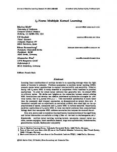
Figure 1: Single hidden layer feedforward networks.

performance. These advantages are attributed to the fact that ELM randomly generates the weights between input layer and hidden layer and uses a least squares method to learn the other weights. For instance, if we consider a SLFNs as Figure 1 illustrating, which has 𝐿 hidden layer nodes and one output layer node, the output function of it is as follows: 𝑓 (x) = h (x) 𝛽,

(1)

where 𝛽 is the weights between hidden layer and output layers and h(x) = [𝐺(a1 , 𝑏1 , x), . . . , 𝐺(a𝐿 , 𝑏𝐿 , x)] is the value vector of hidden layer that maps original features into a new feature space. Different from other SLFNs training methods, ELM can use any h(x), in which 𝐺(a𝑖 , 𝑏, x) is a nonlinear piecewise continuous function, such as sigmoid function and Gaussian function. Moreover, a, the weights between input layer and hidden layer, and 𝑏, the bias of hidden nodes, can be randomly chosen based on any continuous probability distribution in ELM. Thus, the only parameter that ELM must learn is 𝛽. ELM learns 𝛽 through solving the following optimization problem [8]: min 𝛽

1 󵄩󵄩 󵄩󵄩2 1 𝑁 2 󵄩𝛽󵄩 + 𝐶∑𝜉𝑖 2󵄩 󵄩 2 𝑖=1

s.t. h (x𝑖 ) 𝛽 = 𝑦𝑖 − 𝜉𝑖 ,

(2) 𝑖 = 1, . . . , 𝑁,

where {x𝑖 , 𝑦𝑖 } is training samples. According to KKT theorem, 𝛽 can be calculated from

2. Related Work Our proposed method is extended from ELM, specifically, kernel based ELM. In this section, we briefly introduce ELM and kernel based ELM.

.. .

𝛽=(

−1 I + H⊤ H) H⊤ Y 𝐶

(3)

−1 I + HH⊤ ) Y, 𝐶

(4)

or 𝛽 = H⊤ (

where H = [h(x1 ), . . . , h(x𝑁)]⊤ and Y = [𝑦1 , . . . , 𝑦𝑁]⊤ . One can use (3) for the case where the number of training samples is huge, that is, 𝑁 ≫ 𝐿, and use (4) on the contrary, that is, 𝑁 ≪ 𝐿.


3

2.2. Kernel Based Extreme Learning Machine. Kernel method can be easily introduced into ELM. Specifically, ELM kernel 𝐾 can be derived from ELM feature mapping function h(x) as follows: K = HH⊤ : 𝐾𝑖,𝑗 = 𝑘 (x𝑖 , x𝑗 ) = ℎ (x𝑖 ) ⋅ ℎ (x𝑗 ) .

(5)

Therefore, ELM output function can be written as follows: ⊤

𝑘(x, x1 ) −1 I [ .. ] 𝑓 (x) = [ . ] ( + K) Y. 𝐶 [𝑘(x, x𝑁)]

(6)

In this case, users do not have to know the h(x) or set the number of hidden nodes 𝐿, that is, the dimension of ELM feature space.

3. Distance Based Multiple Kernel ELM Since the goal of multiple kernel learning is to construct a new kernel that more suitable for problem processing, the nature of “good” kernel must be considered. Generally, kernel can be seen as a measure of similarity. Each entry in a kernel matrix represents a similarity of two corresponding samples. From this point of view, a “good” kernel can display the true similarity of sample pairs. In other words, if two sample pairs have similar similarity, their corresponding value in the “good” kernel will also be similar. To this end, we propose distance based multiple kernel ELM. It measures similarities of sample pairs by their “label distance” that will be defined in the following part and uses this information to construct a “good” kernel. DBMK-ELM is a kind of two-stage multiple kernel learning method. In the first stage, it learns a new kernel. In the second stage, it uses the new kernel in kernel based ELM. 3.1. Label Distance. We first define the “label distance”. As a significant part of training samples, the label contains class information in the classification case and dependent variable information in the regression case, which can be used to measure true similarity between samples. Considering different label meaning between classification and regression, we discuss “label distance” in these two cases separately. In the classification case, the label means the class that a sample belongs to and samples can be seen as similar when they are in the same class. In other words, if two samples have the same label, they can be seen as similar. On the contrary, if two samples have different labels, they can be seen as different. However, in this case, it is difficult to discriminate how different two samples are, because the difference between classes is not clear. Therefore, label distance is defined to 0 if two samples have the same label and defined to 1 if two samples have different labels. Formally, we define label distance 𝑔(𝑦, 𝑦󸀠 ) as follows: 0 𝑦 = 𝑦󸀠 𝑔 (𝑦, 𝑦󸀠 ) = { 1 𝑦 = ̸ 𝑦󸀠 .

(7)

In the regression case, the label means the value of the dependent variable. Typically, the similarity of samples

is directly represented in the difference of their values of dependent variable in regression cases, for example, pollution prediction, housing number prediction, and stock price prediction, to name just a few. Thus, label distance can be defined as distance between two values of the dependent variable. Admittedly, various measurements can be used to measure this distance, but Euclidean distance is used in this paper. We, in the regression case, formally define the label distance 𝑔(𝑦, 𝑦󸀠 ) as follows: 󵄨 󵄨 (8) 𝑔 (𝑦, 𝑦󸀠 ) = 󵄨󵄨󵄨󵄨𝑦 − 𝑦󸀠 󵄨󵄨󵄨󵄨 . 3.2. Multiple Kernel Learning Based on Distance. Since label distance has been defined above, the distance information can be used to guide the new kernel learning. In this subsection, we show how does DBMK-ELM perform multiple kernel learning based on distance. As we discussed, the new optimal kernel can be seen as a linear combination of base kernels. Therefore, the goal of distance based multiple kernel learning (DBMK) is to learn the combination coefficients of base kernels from which a new kernel that each entry value is coincident to the label distance of the corresponding sample pair can be generated. Considering values of the same entry in each base kernels, corresponding to the same sample pair, if they are seen as input features and the label distance of the same sample pair is seen as output value, the DBMK can be transformed to the regression problem, in which parameters of the regressor are the combination coefficients that need to be learned. To this end, DBMK learns the combination coefficients following the next two steps. Firstly, it reconstructs a new sample space, named K-space, in which each sample corresponds to a sample pair in the original sample space, based on multiple base kernels and label distance of sample pairs. Secondly, it solves a regression problem in this new space to find combination coefficients of kernels. After this two steps, DBMK-ELM can obtain the new optimal kernel through combining the base kernels using learned combination coefficients. For machine learning problems, including classification and regression, if training samples (x, 𝑦) are drawn from a distribution 𝑃 over X × Y ⊂ R𝑛 × R and 𝑝 base kernels, which must satisfy the positive semidefinite condition, are generated by a set of kernel functions {𝑘1 (⋅, ⋅), . . . , 𝑘𝑝 (⋅, ⋅)} and denoted as K1 , . . . , K𝑝 with K𝑖 : X×X → R, DMKL-ELM reconstructs the K-space as {zxx󸀠 , 𝑡𝑦𝑦󸀠 | ((x, 𝑦), (x󸀠 , 𝑦󸀠 ) ∼ 𝑃 × 𝑃) ⊂ R𝑝 × R} where zxx󸀠 = (𝑘1 (x, x󸀠 ) , . . . , 𝑘𝑝 (x, x󸀠 )) , 𝑡𝑦𝑦󸀠 = 𝑔 (𝑦, 𝑦󸀠 ) .

(9)

In the K-space, DBMK-ELM learns the combination coefficients through solving a regression problem. In this problem, the training samples are (z, 𝑡), the whole samples in K-space, in which input feature vector is z and the output label is 𝑡. Though numbers of methods can be used to solve the regression problem, DBMK-ELM applies an ℓ2 -norm regularization least squares linear regression, which is similar to ELM output weight learning, to solve it, considering a fast

4


training speed. This method aims to minimize the training error and the norm of combination coefficients at the same time. If K-space has 𝑁 samples, the optimization objective function of it can be formalized as follows: min 𝜇

1 󵄩󵄩 󵄩󵄩2 1 𝑁 2 󵄩𝜇󵄩 + 𝐶∑𝜉𝑖 2󵄩 󵄩 2 𝑖=1

s.t. 𝑧𝑖 𝜇 = 𝑡𝑖 − 𝜉𝑖 ,

⊤

(10)

𝑖 = 1, . . . , 𝑁,

where 𝜇 is the combination coefficients that DBMK-ELM needs to learn, (z𝑖 , 𝑡𝑖 ) corresponds to the 𝑖th sample in K-space, 𝜉𝑖 represents the training error generated by 𝑖th sample, and 𝐶 is a trade-off parameter. Using KKT theorem, solving (10) is equivalent to solving its dual optimization problem: 𝐿=

1 󵄩󵄩 󵄩󵄩2 1 𝑁 2 𝑁 󵄩𝜇󵄩 + 𝐶∑𝜉𝑖 − ∑𝛼𝑖 (z𝑖 𝜇 − 𝑡𝑖 + 𝜉𝑖 ) , 2󵄩 󵄩 2 𝑖=1 𝑖=1

(11)

where 𝛼𝑖 is the Lagrange multiplier corresponding to the 𝑖th sample. In this case, KKT optimality conditions can be written as follows: 𝑁 𝜕𝐿 = 0 󳨀→ 𝜇 = ∑𝛼𝑖 z⊤𝑖 = Z⊤ 𝛼 𝜕𝜇 𝑖=1

𝜕𝐿 = 0 󳨀→ 𝛼𝑖 = 𝐶𝜉𝑖 , 𝜕𝜉𝑖

𝑖 = 1, . . . , 𝑁

𝜕𝐿 = 0 󳨀→ z𝑖 𝜇 − 𝑡𝑖 + 𝜉𝑖 = 0, 𝜕𝛼𝑖

(12)

𝑖 = 1, . . . , 𝑁,

where Z = [z1 , . . . , z𝑁]⊤ and 𝛼 = [𝛼1 , . . . , 𝛼𝑁]⊤ . According to (12), we have −1 I + ZZ⊤ ) T 𝐶

(13)

−1 I + Z⊤ Z) Z⊤ T, 𝐶

(14)

𝜇 = Z⊤ ( and equally 𝜇=(

3.3. Multiple Kernel Extreme Learning Machine. In the second stage, DBMK-ELM uses the learned new kernel, in which multiple kernel information is included, in the kernel based ELM in both the training and testing case. Therefore, the output function of DBMK-ELM can be written as follows:

where T = [𝑡1 , . . . , 𝑡𝑁]⊤ in both equations above. We can use (13) to calculate 𝜇 when the number of training samples in K-space is not huge and use (14) in the opposite case to speed up the computation. Finally, DBMK-ELM obtains the new optimal kernel by combining base kernels according to 𝜇 as follows: 𝐾new = 𝜇1 𝐾1 + ⋅ ⋅ ⋅ + 𝜇𝑝 𝐾𝑝 .

(15)

Similarily, for each two sample pair (𝑥𝑖 , 𝑥𝑗 ), their new optimal kernel function can be written as follows: 𝑘new (𝑥𝑖 , 𝑥𝑗 ) = 𝜇1 𝑘1 (𝑥𝑖 , 𝑥𝑗 ) + ⋅ ⋅ ⋅ + 𝜇𝑝 𝑘𝑝 (𝑥𝑖 , 𝑥𝑗 ) .

(16)

𝑘new (x, x1 ) −1 I ] [ .. 𝑓 (x) = [ ] ( + Knew ) Y, . 𝐶 [𝑘new (x, x𝑁)]

(17)

where Y = [𝑦1 , . . . , 𝑦𝑁]⊤ . At this point, DBMKL-ELM can successfully deal with the classification and regression problem benefitting from multiple kernel at a fast speed. For a classification or regression problem, DBMK-ELM first learns the combination coefficients of pregenerated base kernels using (13) or (14). Then, it calculates a new optimal kernel by (15). Finally, the result of the problem can be obtained by (17). The algorithm of DBMK-ELM can be illustrated as Algorithm 1. 3.4. Connected to TS-MKL. A previous successful multiple kernel learning approach TS-MKL (two-stage multiple kernel learning) [21] also follows the idea that uses the label information to learn kernel. It denotes +1 for the same label and −1 for different labels to construct its target labels. This is very similar to DBMK-ELM label distance in the classification case. The experimental results show that this method can find a really good kernel that achieves the stateof-the-art classification performance. However, TS-MKL can only solve the classification problem. DBMK-ELM does not just consider the difference between classes but uses label distance to measure the similarity of a sample pair. In this way, DBMK-ELM not only adapts to the classification problem but also adapts to the regression problem.

4. Experiments In this section, we first compare DBMK-ELM to several methods in both classification and regression benchmarks using pregenerated kernels. In order to verify DBMK-ELM performance on multiple kernel learning, SimpleMKL [16] and unweighted sum of kernel methods (UW) have been compared. Meanwhile, we also compare DBMK-ELM with basic kernel based ELM [8] in which the best kernel in base kernels has been used. Then, we compare the classification accuracy between DBMK-ELM and ELM in multiple kernel classification benchmarks, in which different kernels are generated from different channels, in order to demonstrate the ability for multisource data fusion of DBMK-ELM. In addition, we compare DBMK-ELM with the state-of-theart multiple kernel extreme learning machine, namely, the ℓ1 -MK-ELM and the radius-incorporated MK-ELM (R-MKELM) [23], in classification benchmark mentioned above, since these two methods can only suit classification cases. Finally, we conduct parameter sensitivity test for DBMKELM. 4.1. Benchmark Data Sets. We choose 12 classification benchmark data sets including ionosphere, sonar, wdbc, wpbc,


5

Input: The set of training samples, (Xtrn , Ytrn ); The set of testing samples, (Xtst , Ytst ); Output: the output vector of DBMK-ELM, o; (1) Pre-generate several different positive semi-definite base kernels 𝐾1 , . . . , 𝐾𝑝 for training samples (Xtrn , Ytrn ); (2) Reconstruct new sample space for K1 , . . . , K𝑝 using (9) and get new samples (Z, 𝑡); (3) Learn base kernel combination coefficients 𝜇 by (13) or (14); (4) Construct the new optimal kernel by (15) and (16); (5) Calculate the output o using (17) for each sample (x𝑖 , 𝑦𝑖 ) in testing set (Xtst , Ytst ); (6) return o; Algorithm 1: Our proposed DBMK-ELM.

Table 1: Summary of the classification problems data sets. Datasets Ionosphere Sonar wdbc wpbc Breast Glass Wine

Table 2: Summary of the regression problems data sets.

Number of training set

Number of testing set

Number of features

Number of classes

Datasets



Number of features

234 138 379 129 70 142 118

117 70 190 65 36 72 60

34 60 30 33 9 9 13

2 2 2 2 6 6 3

PM10 Bodyfat Housing Pollution Spacega Servo Yacht

333 168 337 40 666 111 205

167 84 169 50 333 56 103

7 14 13 15 6 4 6

breast, glass, and wine from UCI Machine Learning Repository [24]. Table 1 shows the number of training samples, testing samples, features, and classes in these data sets. The regression benchmark data sets used in this experiment are taken from UCI Machine Learning Repository [24] and Statlib [25]. These sets include PM10 [25], bodyfat [25], housing [24], pollution [25], spacega [25], servo [24], and yacht [24]. We display the information, including the number of training samples, testing samples, and features of these sets in Table 2. Three multiple kernel classification benchmarks from bioinformatics data sets are selected in our experiment. The first of them is the original plant data set of TargetP [26]. The others are PsortPos and PsortNeg [27] that both for bacterial protein locations problem. We show the number of training samples, testing samples, kernels, and classes in these data sets on Table 3. For each data set, we randomly select two-thirds of the data samples as training data and the rest as testing data. We repeat this procedure 20 times for each data set and obtain 20 partitions of original data. All algorithms in the experiment are evaluated on each partition and the averaged results are reported for each benchmark. 4.2. Parameters Setting and Evaluation Criteria. For both classification and regression benchmark data sets, we generate 23 kernels on full feature vector, including 20 Gaussian 2 kernels (𝑒−𝛾‖x𝑖 −x𝑗 ‖ ) with 𝛾 = {2−10 , 2−9 , . . . , 29 }, 3 polynomial

Table 3: Summary of the multiple kernel classification benchmark data sets. Datasets



Number of kernels

Number of classes

Plant PsortPos PsortNeg

627 361 963

313 180 481

69 69 69

4 4 5

kernels of degrees 1, 2, and 3. For the kernel based ELM [8], we test all the 23 kernels generated above and display the best result of them in our experiments according to the testing accuracy. For all algorithms, the regulation parameter 𝐶 is selected from {10−1 , 100 , . . . , 103 } via 3-fold cross validation on training data. We select accuracy and computational efficiency as the performance evaluation criteria. The accuracy means the classification accuracy rate in testing data for classification problems or the mean square error (MSE) in testing data for regression problems. In addition, for the regression problem, sample labels have been normalized to [−1, 1]. For all cases, the computational efficiency is evaluated by the training time. The reported results for each benchmark include the mean value and the standard deviation of criteria in 20 partitions. In order to measure the statistical significance for the accuracy improvement, we further use the paired student’s t-test, in which 𝑃 value means the probability that

6

Mathematical Problems in Engineering Table 4: Classification case: classification accuracy (%). Boldface means no statistical difference from the best one (𝑃 val ≥ 0.05).

Data Ionosphere Sonar wdbc wpbc Breast Glass Wine AVG

DBMK-ELM 94.23 ± 1.44 (0.25) 84.71 ± 5.35 (1.00) 97.13 ± 1.32 (0.70) 77.38 ± 3.57 (1.00) 69.03 ± 5.65 (1.00) 71.04 ± 4.31 (1.00) 97.92 ± 1.94 (0.20) 84.49

SimpleMKL [16] 94.23 ± 1.96 (0.22) 84.36 ± 5.51 (0.62) 97.05 ± 1.11 (0.44) 75.31 ± 3.55 (0.01) 65.56 ± 7.45 (0.01) 54.86 ± 4.22 (0.00) 98.33 ± 1.71 (1.00) 81.39

ℓ1 -MK-ELM [23] 94.62 ± 1.78 (1.00) 84.64 ± 5.75 (0.90) 97.16 ± 1.19 (0.74) 75.23 ± 3.56 (0.00) 65.83 ± 8.26 (0.02) 68.61 ± 5.71 (0.01) 98.17 ± 2.22 (0.61) 83.47

R-MK-ELM [23] 94.32 ± 1.82 (0.23) 82.57 ± 5.22 (0.00) 97.08 ± 1.45 (0.49) 75.46 ± 3.91 (0.02) 67.08 ± 7.34 (0.04) 70.14 ± 4.33 (0.15) 98.00 ± 2.45 (0.41) 83.52

ELM [8] 90.38 ± 2.88 (0.00) 84.21 ± 4.71 (0.56) 97.21 ± 1.26 (1.00) 76.23 ± 3.72 (0.16) 65.83 ± 7.55 (0.03) 67.57 ± 5.18 (0.01) 97.58 ± 2.13 (0.02) 82.72

UW 93.33 ± 1.93 (0.00) 81.57 ± 5.16 (0.00) 97.11 ± 1.41 (0.62) 76.31 ± 4.16 (0.18) 66.94 ± 6.98 (0.00) 69.31 ± 5.46 (0.08) 98.00 ± 2.27 0.43 83.22

Table 5: Classification case: classification training time (s). Data Ionosphere Sonar wdbc wpbc Breast Glass Wine AVG

DBMK-ELM 0.0210 ± 0.0016 0.0063 ± 0.0006 0.0580 ± 0.0051 0.0061 ± 0.0006 0.0016 ± 0.0004 0.0083 ± 0.0016 0.0063 ± 0.0014 0.0153

SimpleMKL [16] 0.8216 ± 0.4888 0.2919 ± 0.1673 4.2746 ± 4.2881 0.3777 ± 0.3230 13.5007 ± 16.8849 6.5990 ± 16.2960 1.2676 ± 0.7903 3.8762

ℓ1 -MK-ELM [23] 0.4115 ± 0.0558 0.2498 ± 0.0396 0.9743 ± 0.2876 0.0685 ± 0.0303 0.1701 ± 0.0405 0.2948 ± 0.1141 0.2299 ± 0.0387 0.3427

two compared sets come from distributions with an equal mean. Typically, if the 𝑃 value less than 0.05, the compared sets are considered having statistically significant difference. 4.3. Classification Performance. The classification accuracy of different methods is shown in Table 4. The content in Table 4 has following meanings, the first part is the mean ± standard deviation and the second part is the 𝑃 value calculated by the paired Student’s 𝑡-test. The bold value in each cell of Table 4 represents the highest accuracy and those having no significant difference compared with the highest one. We also show the classification training time in Table 5, which presents as the mean ± standard deviation. As we can see from Table 4, DBMK-ELM achieves the highest correct classification rate or has no significant different compared with the best one. Meanwhile, the results in Table 5 prove that the time cost of this approach is significantly lower than SimpleMKL, ℓ1 -MK-ELM, and RMK-ELM. 4.4. Regression Performance. The regression accuracy of different methods is shown in Table 6 with the same representation of Table 4. And the regression training time is shown in Table 7.

R-MK-ELM [23] 1.9217 ± 0.0419 0.7698 ± 0.0242 6.4733 ± 0.2250 0.6542 ± 0.0202 0.3024 ± 0.0214 0.7010 ± 0.0631 0.6000 ± 0.0168 1.632

ELM [8] 0.0009 ± 0.0001 0.0003 ± 0.0001 0.0023 ± 0.0004 0.0004 ± 0.0001 0.0003 ± 0.0002 0.0005 ± 0.0001 0.0004 ± 0.0002 0.0007

UW 0.0009 ± 0.0001 0.0003 ± 0.0000 0.0024 ± 0.0004 0.0004 ± 0.0001 0.0002 ± 0.0001 0.0004 ± 0.0001 0.0004 ± 0.0001 0.0007

In this case, we can see DBMK-ELM has the significant highest regression accuracy compared with other methods. From the time cost point of view, this situation is similar to the classification problem; that is, DBMK-ELM dramatically improved training time compared to SimpleMKL. 4.5. Multiple Kernel Classification Benchmark Performance. The classification accuracy for multiple kernel classification benchmarks of DBMK-ELM and other methods is shown in Table 8. And the multiple kernel classification training time is shown in Table 9. From the results, we can see DBMKELM significantly better than ELM. That means DBMK-ELM has the ability to perform multisource data fusion, thereby improving the performance of ELM. The DBMK-ELM is better than the state-of-the-art multiple kernel extreme learning machine in this case regarding the classification accuracy and the training time. 4.6. Parameter Sensitivity Test. In our proposed DBMKELM, there are two regularization parameters need to be set. In order to describe more clearly, we use 𝐶1 and 𝐶2 represents the regularization parameter in ELM training and multiple kernel learning, respectively. We choose classification data set ionosphere and regression data set yacht to test parameter sensitivity. For each data set, we set a wide range of 𝐶1 and


7

Table 6: Regression case: regression accuracy (%). Boldface means no statistical difference from the best one (𝑃 val ≥ 0.05). Data PM10 Bodyfat Housing Pollution Servo Spacega Yacht AVG

DBMK-ELM 0.3242 ± 0.0171 (1.00) 0.0559 ± 0.0227 (1.00) 0.1618 ± 0.0256 (1.00) 0.2738 ± 0.0469 (1.00) 0.1926 ± 0.0408 (1.00) 0.1415 ± 0.0073 (1.00) 0.1083 ± 0.0192 (1.00) 0.1797

SimpleMKL [16] 0.3347 ± 0.0152 (0.00) 0.0898 ± 0.0264 (0.00) 0.2006 ± 0.0430 (0.00) 0.3167 ± 0.0660 (0.00) 0.2121 ± 0.0528 (0.04) 0.1735 ± 0.0136 (0.00) 0.1947 ± 0.0323 (0.00) 0.2174

ELM [8] 0.3305 ± 0.0172 (0.01) 0.0755 ± 0.0254 (0.00) 0.1760 ± 0.0264 (0.00) 0.2767 ± 0.0438 (0.61) 0.2046 ± 0.0396 (0.01) 0.1655 ± 0.0104 (0.00) 0.1839 ± 0.0228 (0.00) 0.2018

UW 0.3256 ± 0.0167 (0.46) 0.1321 ± 0.0246 (0.00) 0.2149 ± 0.0323 (0.00) 0.3110 ± 0.0606 (0.00) 0.2567 ± 0.0379 (0.00) 0.1633 ± 0.0106 (0.00) 0.2420 ± 0.0342 (0.00) 0.2351

Table 7: Regression case: regression training time (s). Data PM10 Bodyfat Housing Pollution Servo Spacega Yacht AVG

DBMK-ELM 0.0430 ± 0.0021 0.0088 ± 0.0009 0.0451 ± 0.0028 0.0004 ± 0.0000 0.0036 ± 0.0004 0.1954 ± 0.0040 0.0152 ± 0.0012 0.0445

SimpleMKL [16] 7.3150 ± 4.2744 5.4048 ± 3.9174 18.3088 ± 11.7929 0.0829 ± 0.0384 1.6819 ± 1.0180 42.0023 ± 54.0406 4.8831 ± 2.3245 11.3827

ELM [8] 0.0010 ± 0.0002 0.0004 ± 0.0001 0.0011 ± 0.0002 0.0001 ± 0.0000 0.0003 ± 0.0003 0.0058 ± 0.0008 0.0005 ± 0.0001 0.0013

UW 0.0010 ± 0.0002 0.0004 ± 0.0001 0.0010 ± 0.0002 0.0001 ± 0.0000 0.0002 ± 0.0000 0.0058 ± 0.0008 0.0005 ± 0.0001 0.0013

Table 8: Multiple kernel classification case: classification accuracy (%). Boldface means no statistical difference from the best one (𝑃 val ≥ 0.05). Data Plant PsortPos PsortNeg AVG

DBMK-ELM 91.82 ± 1.43 (1.00) 87.92 ± 2.03 (1.00) 91.52 ± 0.86 (1.00) 90.42

SimpleMKL [16] 67.38 ± 3.43 (0.00) 80.22 ± 2.91 (0.00) 84.80 ± 1.74 (0.00) 77.47

ℓ1 -MK-ELM [23] 58.85 ± 2.96 (0.00) 70.31 ± 3.35 (0.00) 73.78 ± 1.82 (0.00) 67.64

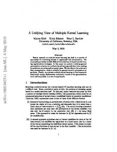
𝐶2. Specifically, we have used 10 different values of 𝐶1 and 10 different values of 𝐶2 from {10−1 , 100 , . . . , 107 , 108 }. For each (𝐶1, 𝐶2) pair, we repeat 20 times on each data set to get the average accuracy. The result of classification case and regression case is shown in Figures 2 and 3, respectively. As can be seen from the results, the performance of DBMK-ELM is not sensitivity while 𝐶1 and 𝐶2 vary within a wide range. 4.7. Discussion. The experimental results have illustrated that DBMK-ELM can achieve a high accuracy with a fast learning speed. However, two issues need to discussed. (1) Why is the learning speed of DBMK-ELM much slower than basic ELM in some cases? The main reason is that there are substantial samples to learn in the K-space, which is constructed in multiple kernel learning step. Specifically, if there are 𝑛 original samples, there will be 𝑛2 corresponding new samples. Therefore, the training time difference between DBMK-ELM and basic ELM will be magnified with the training samples increasing. It may be possible to reduce the

R-MK-ELM [23] 85.32 ± 2.56 (0.00) 84.14 ± 2.12 (0.00) 89.75 ± 1.23 (0.00) 86.40

ELM [8] 78.51 ± 2.23 (0.00) 80.83 ± 2.45 (0.00) 85.87 ± 1.81 (0.00) 81.74

UW 74.79 ± 2.55 (0.00) 81.03 ± 2.69 (0.00) 87.31 ± 1.42 (0.00) 81.04

training time gap between DBMK-ELM and basic ELM if we use sampling techiques in the K-space. (2) In which cases should we use DBMK-ELM? DBMKELM can obtain more accurate results and a faster learning speed compared with traditional multiple kernel learning method, SimpleMKL. Despite the fact that it is much better than other multiple kernel learning methods, DBMK-ELM has more time cost compared with basic ELM method. In this way, a trade-off between accuracy and time cost is needed. The experimental results show that DBMK-ELM significantly improves testing accuracy compared with basic ELM in regression and multisource data fusion problems in most cases. But in the classification case, where kernels are generated from one data source, DBMK-ELM has no significant difference compared with basic ELM in testing accuracy. Therefore, a preferable choice is to apply DBMKELM in regression and multisource data fusion problems and use basic ELM in single data source generated kernel classification problems.

8

Mathematical Problems in Engineering Table 9: Multiple kernel classification case: classification training time (s).

Data Plant PsortPos PsortNeg AVG

DBMK-ELM 0.6545 ± 0.0272 0.2062 ± 0.0124 1.5343 ± 0.1060 0.7983

SimpleMKL [16] 9.1479 ± 0.6296 2.3172 ± 0.2031 25.5086 ± 1.1290 12.3246

ℓ1 -MK-ELM [23] 4.5658 ± 0.5378 0.8097 ± 0.0893 11.9782 ± 0.7766 5.7846

R-MK-ELM [23] 7.8680 ± 0.6125 2.4892 ± 0.3435 24.7445 ± 1.0424 11.7006

ELM [8] 0.0064 ± 0.0006 0.0019 ± 0.0005 0.0187 ± 0.0009 0.0090

UW 0.0065 ± 0.0006 0.0017 ± 0.0003 0.0187 ± 0.0011 0.0090

Classification accuracy (%)

Acknowledgments 100 90 80 70 100 90 80 70 109

This work was supported by the National Natural Science Foundation of China (Project nos. 60970034, 61170287, and 61232016), the National Basic Research Program of China (973) under Grant no. 2014CB340303, and the Hunan Provincial Science and Technology Planning Project of China (Project no. 2012FJ4269). 107

105 3 10 101 C2

1 10−1 10−1 10

105 10 C1 3

107

109

References

Figure 2: Classification case: performances of DBMK-ELM with different parameters on the ionosphere data set.

[1] J. Yin, E. Zhu, X. Yang, G. Zhang, and C. Hu, “Two steps for fingerprint segmentation,” Image and Vision Computing, vol. 25, no. 9, pp. 1391–1403, 2007.

Regression accuracy

[2] C. Zhu, J. Yin, and Q. Li, “A stock decision support system based on DBNs,” Journal of Computational Information Systems, vol. 10, no. 2, pp. 883–893, 2014. 0.8 0.6 0.4 0.2 0 109

[3] D. E. Rumelhart, G. E. Hinton, and R. J. Williams, “Learning representations by back-propagating errors,” Nature, vol. 323, no. 6088, pp. 533–536, 1986. [4] V. Vapnik, The Nature of Statistical Learning Theory, Springer, 2000. 107 105 103 101 −1 10 C2

10−1 10

1

5 10 10 C1 3

107

109

Figure 3: Regression case: performances of DBMK-ELM with different parameters on the yacht data set.

5. Conclusion In this paper, we have proposed DBMK-ELM, a new multiple kernel based ELM, to extend the basic kernel based ELM. The proposed multiple kernel learning method can unify classification and regression problems. Moreover, DBMKELM is able to learn from multiple kernels at an extremely fast speed. Experimental results show that DBMK-ELM achieves a significant performance enhancement, in terms of the accuracy and the time cost in both classification and regression problems. In future, we will consider how to define a better distance among different classes and how to extend DBMK-ELM to the semisupervised learning problem.

[5] G.-B. Huang, Q.-Y. Zhu, and C.-K. Siew, “Extreme learning machine: a new learning scheme of feedforward neural networks,” in Proceedings of the IEEE International Joint Conference on Neural Networks, vol. 2, pp. 985–990, July 2004. [6] G.-B. Huang, Q.-Y. Zhu, and C.-K. Siew, “Extreme learning machine: theory and applications,” Neurocomputing, vol. 70, no. 1–3, pp. 489–501, 2006. [7] Y. Wang, F. Cao, and Y. Yuan, “A study on effectiveness of extreme learning machine,” Neurocomputing, vol. 74, no. 16, pp. 2483–2490, 2011. [8] G.-B. Huang, H. Zhou, X. Ding, and R. Zhang, “Extreme learning machine for regression and multiclass classification,” IEEE Transactions on Systems, Man, and Cybernetics B: Cybernetics, vol. 42, no. 2, pp. 513–529, 2012. [9] Y. Yuan, Y. Wang, and F. Cao, “Optimization approximation solution for regression problem based on extreme learning machine,” Neurocomputing, vol. 74, no. 16, pp. 2475–2482, 2011. [10] J. Lin, J. Yin, Z. Cai, Q. Liu, K. Li, and V. Leung, “A secure and practical mechanism of outsourcing extreme learning machine in cloud computing,” IEEE Intelligent Systems, vol. 28, no. 6, pp. 35–38, 2013.

Conflict of Interests

[11] N.-Y. Liang, G.-B. Huang, P. Saratchandran, and N. Sundararajan, “A fast and accurate online sequential learning algorithm for feedforward networks,” IEEE Transactions on Neural Networks, vol. 17, no. 6, pp. 1411–1423, 2006.

The authors declare that there is no conflict of interests regarding the publication of this paper.

[12] J. Cao, Z. Lin, G.-B. Huang, and N. Liu, “Voting based extreme learning machine,” Information Sciences, vol. 185, no. 1, pp. 66– 77, 2012.

Mathematical Problems in Engineering [13] W. Zong, G.-B. Huang, and Y. Chen, “Weighted extreme learning machine for imbalance learning,” Neurocomputing, vol. 101, pp. 229–242, 2013. [14] Z. Bai, G. B. Huang, D. Wang, H. Wang, and M. B. Westover, “Sparse extreme learning machine for classification,” IEEE Transactions on Cybernetics, vol. 44, no. 10, pp. 1858–1870, 2014. [15] G. R. Lanckriet, N. Cristianini, P. Bartlett, L. El Ghaoui, and M. I. Jordan, “Learning the kernel matrix with semidefinite programming,” Journal of Machine Learning Research, vol. 5, pp. 27–72, 2004. [16] A. Rakotomamonjy, F. R. Bach, S. Canu, and Y. Grandvalet, “SimpleMKL,” Journal of Machine Learning Research (JMLR), vol. 9, pp. 2491–2521, 2008. [17] M. Kloft, U. Brefeld, S. Sonnenburg, and A. Zien, “𝐿 𝑝 -norm multiple kernel learning,” The Journal of Machine Learning Research, vol. 12, pp. 953–997, 2011. [18] X. Liu, L. Wang, J. Yin, and L. Liu, “Incorporation of radiusinfo can be simple with SimpleMKL,” Neurocomputing, vol. 89, pp. 30–38, 2012. [19] X. Liu, L. Wang, J. Zhang, and J. Yin, “Sample-adaptive multiple kernel learning,” AAAI, 2014. [20] N. Cristianini, J. Shawe-Taylor, A. Elisseeff, and J. S. Kandola, “On kernel-target alignment,” in Advances in Neural Information Processing Systems, vol. 14, pp. 367–373, MIT Press, 2002, http://papers.nips.cc/paper/1946-on-kernel-targetalignment.pdf. [21] A. Kumar, A. Niculescu-Mizil, K. Kavukcoglu, and H. Daum´e, “A binary classification framework for two-stage multiple kernel learning,” in Proceedings of the 29th International Conference on Machine Learning (ICML ’12), pp. 1295–1302, July 2012. [22] L.-J. Su and M. Yao, “Extreme learning machine with multiple kernels,” in Proceedings of the 10th IEEE International Conference on Control and Automation (ICCA ’13), pp. 424–429, June 2013. [23] X. Liu, L. Wang, G. B. Huang, J. Zhang, and J. Yin, “Multiple kernel extreme learning machine,” Neurocomputing, vol. 149, part A, pp. 253–264, 2015. [24] K. Bache and M. Lichman, UCI machine learning repository, 2013, http://archive.ics.uci.edu/ml. [25] http://lib.stat.cmu.edu/datasets/. [26] O. Emanuelsson, H. Nielsen, S. Brunak, and G. von Heijne, “Predicting subcellular localization of proteins based on their N-terminal amino acid sequence,” Journal of Molecular Biology, vol. 300, no. 4, pp. 1005–1016, 2000. [27] J. L. Gardy, M. R. Laird, F. Chen et al., “PSORTb v.2.0: expanded prediction of bacterial protein subcellular localization and insights gained from comparative proteome analysis,” Bioinformatics, vol. 21, no. 5, pp. 617–623, 2005.

9

Advances in

Operations Research Hindawi Publishing Corporation http://www.hindawi.com

Volume 2014

Advances in

Decision Sciences Hindawi Publishing Corporation http://www.hindawi.com

Volume 2014

Journal of

Applied Mathematics

Algebra

Hindawi Publishing Corporation http://www.hindawi.com


Volume 2014

Journal of

Probability and Statistics Volume 2014

The Scientific World Journal Hindawi Publishing Corporation http://www.hindawi.com


Volume 2014

International Journal of

Differential Equations Hindawi Publishing Corporation http://www.hindawi.com

Volume 2014

Volume 2014

Submit your manuscripts at http://www.hindawi.com International Journal of

Advances in

Combinatorics Hindawi Publishing Corporation http://www.hindawi.com

Mathematical Physics Hindawi Publishing Corporation http://www.hindawi.com

Volume 2014

Journal of

Complex Analysis Hindawi Publishing Corporation http://www.hindawi.com

Volume 2014

International Journal of Mathematics and Mathematical Sciences


Journal of

Mathematics Hindawi Publishing Corporation http://www.hindawi.com

Volume 2014


Volume 2014

Volume 2014


Volume 2014

Discrete Mathematics

Journal of

Volume 2014


Discrete Dynamics in Nature and Society

Journal of

Function Spaces Hindawi Publishing Corporation http://www.hindawi.com

Abstract and Applied Analysis

Volume 2014


Volume 2014


Volume 2014

International Journal of

Journal of

Stochastic Analysis

Optimization



Volume 2014

Volume 2014