MNRAS 000, ??–?? (2016)
Preprint 18 November 2016
Compiled using MNRAS LATEX style file v3.0
Galaxy clustering dependence on the [OII] emission line luminosity in the local Universe Ginevra Favole1? , Sergio A. Rodr´ıguez-Torres2,3,4 †, Johan Comparat2,3,4 ‡, Francisco Prada2,3,5 , Hong Guo6 , Anatoly Klypin7 , Antonio D. Montero-Dorta8 1 European
Space Astronomy Center (ESAC), 3825 Villanueva de la Ca˜ nada, Madrid, Spain de F´ısica Te´ orica (IFT) UAM/CSIC, Universidad Aut´ onoma de Madrid, Cantoblanco, E-28049 Madrid, Spain 3 Campus of International Excellence UAM/CSIC, Cantoblanco, E-28049 Madrid, Spain 4 Departamento de F´ ısica Te´ orica M-8, Universidad Aut´ onoma de Madrid, Cantoblanco, 28049 Madrid, Spain 5 Instituto de Astrof´ ısica de Andaluc´ıa (CSIC), Granada, E-18008, Spain 6 Key Laboratory for Research in Galaxies and Cosmology, Shanghai Astronomical Observatory, Shanghai 200030, China 7 Astronomy Department, New Mexico State University, MSC 4500, P.O. Box 30001, Las Cruces, NM, 880003-8001, USA 8 Department of Physics and Astronomy, University of Utah, UT 84112, USA
arXiv:1611.05457v1 [astro-ph.GA] 16 Nov 2016
2 Instituto
ABSTRACT
We study the galaxy clustering dependence on the [O ii] emission line luminosity in the SDSS DR7 Main galaxy sample at mean redshift z ∼ 0.1. We select volumelimited samples of galaxies with different [O ii] luminosity thresholds and measure their projected, monopole and quadrupole two-point correlation functions. We model these observations using the 1h−1 Gpc MultiDark Planck cosmological simulation and generate light-cones with the SUrvey GenerAtoR algorithm. To interpret our results, we adopt a modified (Sub)Halo Abundance Matching scheme, accounting for the stellar mass incompleteness of the emission line galaxies. The satellite fraction constitutes an extra parameter in this model and allows to optimize the clustering fit on both small and intermediate scales (i.e. rp . 30 h−1 Mpc), with no need of any velocity bias correction. We find that, in the local Universe, the [O ii] luminosity correlates with all the clustering statistics explored and with the galaxy bias. This latter quantity correlates more strongly with the SDSS r-band magnitude than [O ii] luminosity. In conclusion, we propose a straightforward method to produce reliable clustering models, entirely built on the simulation products, which provides robust predictions of the typical ELG host halo masses and satellite fraction values. The SDSS galaxy data, MultiDark mock catalogues and clustering results are made publicly available. Key words: galaxies: distances and redshifts — galaxies: haloes — galaxies: statistics — cosmology: observations — cosmology: theory — large-scale structure of Universe
1
INTRODUCTION
In the last decade, the Sloan Digital Sky Survey (SDSS; York et al. 2000; Gunn et al. 2006; Smee et al. 2013) first, and then the SDSS-III/Baryon Oscillation Spectroscopic Survey (BOSS; Eisenstein et al. 2011; Dawson et al. 2013) have mainly observed luminous red galaxies (LRGs; Eisenstein et al. 2001) up to redshift z ∼ 0.7 to trace the baryon acoustic oscillation feature (BAO; Eisenstein et al. 2005) in their clustering signal and use it as “standard ruler” for cosmological distances. New-generation large-volume spectroscopic surveys, both ground-based as eBOSS (Dawson et al. 2016), DESI (Schlegel et al. 2015), 4MOST (de Jong et al. 2012), Subaru-PFS (Sugai et al. 2015) and space-based as Euclid (Laureijs et al. 2011; Sartoris et al. 2015), have all been designed to probe larger volumes by looking back in
?
E-mail:
[email protected] † Campus de Excelencia Internacional UAM/CSIC Scholar ‡ Severo Ochoa IFT Fellow c 2016 The Authors
time out to z ∼ 2 and to target high-redshift star-forming galaxies with strong nebular emission lines (ELGs) as BAO tracers. For galaxies at the peak of cosmic star formation at z ∼ 2, these emission lines are shifted into the near-infrared which, combined with the intrinsic faintness of the source, makes them difficult to observe using ground-based facilities (Masters et al. 2014). For this reason, relatively few nearinfrared spectra of galaxies at z ∼ 2 that cover all the important rest-frame optical emission lines have been published to date (e.g., Erb et al. 2006, 2010; Hainline et al. 2009; Rigby et al. 2011; Belli et al. 2013; Dom´ınguez et al. 2013). The available near-infrared spectra of star-forming galaxies at z ∼ 2 have revealed differences in comparison with their counterparts in the local Universe (Liu et al. 2008; Newman et al. 2014). For example, star-forming galaxies at z ∼ 2 tend to have higher [O iii]/Hβ ratios at a given [N ii]/Hα ratio compared to local star-forming galaxies. This evidence has been attributed to more extreme interstellar medium conditions, on average, in galaxies at high redshift, possibly as a result of harder ionizing radiation field, different gas vol-
2
Favole et al. 2016
ume filling factors, higher nebular electron densities, AGN activity (Shapley et al. 2005; Brinchmann et al. 2008; Shirazi et al. 2014; Kewley et al. 2013). The clumpy morphology and high velocity dispersions observed in many of these sources (Pettini et al. 2001; Genzel et al. 2008; Law et al. 2009) may support the conjecture that star formation in the early Universe generally occurs in denser and higher pressure environments than those found in local star-forming galaxies. The slitless grim spectroscopy provided by the Wide Field Camera 3 (WFC3) on the Hubble Space Telescope has lead to the discovery of large numbers of star-forming galaxies near the peak of cosmic star formation (Atek et al. 2010). Grism surveys as the WFC3 Infrared Spectroscopic Parallel (WISP; Atek et al. 2010) survey, are ideal to detect low-mass star-forming galaxies at intermediate redshift through their optical emission lines, but they lack of spectral resolution to resolve Hα from [N ii] λ = 6548, 6583 ˚ A or detect line broadening due to AGN activity. The Euclid slitless grim spectroscopic program, with a similar design to WISP, will be able to measure the [N ii]/Hα flux ratio with small enough errors to reliably distinguish narrow-line AGN and star-forming galaxies down to Hα fluxes of ∼ 1.5 × 10⁻¹⁵ erg cm−2 s−1 , over the redshift range 0.7 < z < 2 (Laureijs et al. 2011). Complementing the new generation of ground-based infrared spectrometers of eBOSS and DESI with the Euclid spacebased facility will help to constrain the physical properties of these emission line galaxies at high redshift, and to understand better their formation and evolution processes. In preparation to these near-future experiments, we discuss here how to measure and correctly model the ELG distribution within their host haloes, their clustering properties as a function of the emission line luminosity and its evolution with redshift, using the data currently available. Specifically, we focus our analysis on the SDSS DR7 Main galaxy sample (Strauss et al. 2002; Abazajian et al. 2009) at mean redshift z ∼ 0.1. We select this sample from the New York-Value Added Galaxy catalogue (NYU-VAGC Blanton et al. 2005) and assign [O ii] luminosities by performing a spectroscopic matching to the MPA-JHU DR7 (at http://www.mpa-garching.mpg.de/SDSS/DR7/) release of spectrum measurements. In the merged galaxy population, we select volume-limited samples in different [O ii] luminosity thresholds, where we measure the projected, monopole and quadrupole two-point correlation functions (2PCFs) and model the results in terms of the typical host halo masses and satellite fraction. We adopt a (Sub)Halo Abundance matching (SHAM; Klypin et al. 2010; Trujillo-Gomez et al. 2011) scheme, modified (Rodr´ıguezTorres et al., 2016, in prep.) to account for the ELG stellar mass incompleteness. The method applied is straightforward since entirely built on the simulation products, with no need of introducing any velocity bias (Guo et al. 2015b), and provides reliable predictions of the ELG host halo masses and satellite fraction values, as a function of the [O ii] luminosity. Our galaxy data and mock catalogues, together with the clustering results, are publicly available both on the Skies and Universes database at http://projects.ift.uam-csic.es/skies-universes/ SUwebsite/indexSDSS_OII_mock.html, and as MNRAS online material. The paper is organized as follows: in Section 2 we describe the SDSS data set used and how we assign [O ii] luminosities. In Section 3 we introduce the tools needed to perform our clustering measurements. In Section 4 we present the simula-
tion and the ELG clustering model. In Section 5 we present our ELG clustering results and the correlation between [O ii] luminosity and galaxy bias. We discuss our conclusions and the future plans in Section 6. In what follows, we adopt the Planck et al. (2014) cosmology: Ωm = 0.3071, ΩΛ = 0.6929, h = 0.6777, n = 0.96, σ8 = 0.8228.
2
DATA
We select the SDSS DR7 Main galaxy sample (Strauss et al. 2002) from the NYU-VAGC1 (Blanton et al. 2005) and assign [O ii] emission line fluxes by performing a spectroscopic matching to the MPA-JHU2 DR7 release of spectrum measurements. We consider only MPA-JHU galaxies with good spectra, i.e. with ZWARNING=0. In what follows, the merged galaxy catalogue will be called “MPA-NYU SDSS Main” catalog. Notice that all the galaxies in this sample show [O ii] emission lines, meaning that we do not include any elliptical or quiescent galaxy which could be central for some of the ELGs considered. We compute the [O ii] fluxes as F = Fc × |EQW |, where Fc is the line flux continuum and EQW is equivalent width of the MPA-JHU lines. In the case of line doublets emitting two different wavelengths as [O ii], the flux considered is the cumulative flux of both lines. Following Hopkins et al. (2003), we correct these fluxes for extinction using Schlegel et al. (1998) E(B − V ) dust maps and Calzetti et al. (2000) law to obtain: corr Fext [erg s−1 cm−2 ] = F×10−0.4Aλ = F×10−0.4E(B−V)k(λobs ) . (1) In the equation above, the quantity k(λobs ) is the reddening curve (Calzetti et al. 2000), λobs = λem (1+z) is the observed wavelength and λem is the emitted one. The observed ELG luminosity is then recovered from the flux as (Hopkins et al. 2003)
Lobs [erg s−1 ] = 4πD2L 10−0.4(mp −mfib ) Fcorr ext ,
(2)
where DL is the luminosity distance depending on redshift and cosmology. In Eq. 2, the exponent is the aperture correction accounting that only the portion of the flux “through the fiber” will be detected by the SDSS spectrograph – fibers in SDSS have an aperture of 3” (Strauss et al. 2002). This correction implicitly assumes that the emission measured through the fiber is characteristic of the whole galaxy and that the star formation is uniformly distributed over the galaxy. The term mp is the petrosian magnitude in the desired band-pass filter representing the total galaxy flux and mf ib is the fiber magnitude derived from a photometric measurement of the magnitude in an aperture the size of the fiber and corrected for seeing effects. In the SDSS ugriz (Gunn et al. 1998; Fukugita et al. 1996) optical photometric system, the [O ii] (λλ3726, 3729) doublet lies in the u-band. The observed [O ii] emission line luminosity of the NYUMPA SDSS Main galaxies in the redshift range 0.02 < z < 0.22 is displayed in the left panel of Figure 1. In the right panel we show the (g − r) [O ii] ELG color as a function of the SDSS r-band absolute magnitude, which is in agreement with the “bluer” and “bluest” subsamples in Zehavi et al. (2011). Since the SDSS DR7 spectra are combined from three or more individual exposures
1 2
http://cosmo.nyu.edu/blanton/vagc/ http://www.mpa-garching.mpg.de/SDSS/DR7/ MNRAS 000, ??–?? (2016)
[O ii] ELG clustering at z ∼ 0.1 of 15 minutes each (see http://classic.sdss.org/dr7/ products/spectra/), corresponding to typical [O ii] fluxes of ∼ 10−16 erg cm−2 s−1 (Comparat et al. 2015), we impose a conservative limit rejecting all galaxies with [O ii] flux lower than 3 × 10⁻¹⁶ erg cm−2 s−1 (black line in Figure 1) and remain with a sample of about 427,000 [O ii] ELGs. To investigate the ELG clustering dependence on the [O ii] luminosity, we select several volume-limited samples in L[OII] thresholds and show them as colored squares in Figure 1. The specific cuts to obtain them are reported in Table 1.
3
CLUSTERING MEASUREMENTS
We measure the projected, monopole and quadrupole twopoint correlation functions of the NYU-MPA SDSS Main volume-limited samples using the Landy-Szalay estimator (Landy & Szalay 1993), for which we build suitable randoms including the angular and radial footprint of the data samples. We take into account the variation of the completeness across the sky by downsampling the NYU-VAGC random catalogue with equal surface density in a random fashion using the completeness as a probability function. We then shuffle the (RA, DEC) random coordinates by sorting them with respect to a random flag, and assign the observed redshifts (Anderson et al. 2014). To correct for angular incompleteness, we weight each object in the real and random catalogues by wang , which is defined as the inverse of the SDSS sector completeness. Since the minimum angular distance allowed between the SDSS optical fiber is 55” (i.e. rp ∼ 0.13 h−1 Mpc at z¯ = 0.1), we limit the measurements to scales larger than that and upweight by one Ross et al. (2012) the fiber collision (Zehavi et al. 2002; Masjedi et al. 2006) weight, wf c , of the nearest neighbor of the collided galaxy. Because we use volume-limited samples, we do not need to apply any radial weight. We combine the corrections above into a total weight (S´ anchez et al. 2012) of wtot = wfc wang . To estimate the errors on our clustering measurements we perform 200 jackknife (e.g., Turkey 1958; Norberg et al. 2011; Ross et al. 2012; Anderson et al. 2012) re-samplings.
4
SIMULATION AND MODELING
We model the ELG clustering measurements using the MultiDark3 (MDPL; Klypin et al. 2016) N-body cosmological simulation with Planck cosmology (Planck et al. 2014). The simulation box is 1 h−1 Gpc on a side, with 38403 particles and a mass resolution of 1.51 × 10⁹ h−1 M . It represents the best compromise between resolution and volume available to date. We apply the SUrvey GenerAtoR (SUGAR; Rodr´ıguez-Torres et al. 2016) algorithm to the MultiDark ROCKSTAR (Behroozi et al. 2013) snapshots in the redshift range 0.02 < z < 0.22 to produce suitable light-cones with about twice the area of the data (i.e., ∼ 12, 000 deg2 ) to reduce the effect of cosmic variance. The advantage of using a light-cone instead of a single simulation snapshot at the mean redshift of the sample is that it includes the redshift evolution. In addition, it accounts for those volume
3
https://www.cosmosim.org
MNRAS 000, ??–?? (2016)
3
effects (cosmic variance and galaxy number density fluctuations) that are observed in the data and a single simulation snapshot cannot capture. The disadvantage of using a light-cone, however, is its reduced volume: from a simulation box of 1 h−3 Gpc3 , the maximum light-cone aperture achieved corresponds to only 1/50 of the original volume, that is about ∼ 0.02 h−3 Gpc3 . This limitation makes this model less accurate on larger scales, therefore we focus our analysis at rp . 30 h−1 Mpc. To populate the MDPL lightcones with the galaxies of the SDSS MPA-NYU volumelimited samples, we adopt the modified (Sub)Halo Abundance Matching (SHAM; Klypin et al. 2011; Trujillo-Gomez et al. 2011) prescription proposed by Rodr´ıguez-Torres et al., 2016, in prep., which accounts for the ELG stellar mass incompleteness, similarly to the method presented in Favole et al. (2016a). This SHAM assignment is performed by drawing mocks using two separate (one for central and one for satellites) probability distribution functions that follow a Gaussian shape defined by the mean and 1σ dispersion of the distribution: Vpeak ± σV . The Vpeak parameter is the halo maximum circular velocity over its entire history and represents the SHAM halo proxy. We handle the number of subhaloes in the final mock catalogue by including the fraction of satellites fsat as a model parameter. The Gaussian distribution is then normalized to reach the desired ELG number density in each redshift bin. The best-fit Vpeak ± σV and fsat values we obtain for the [O ii] ELG volume-limited samples are reported in Table 1. For each mock catalog, we also display the most probable (i.e. more representative) or “typical” Vpeak and Mh value, corresponding to the peak of the halo velocity and mass distributions. The difference between the best-fit and typical velocities is due to the fact that for certain Vpeak values we do not have enough haloes to draw from the Gaussian PDF, then the algorithm picks haloes with smaller velocity until the desired number density is achieved. This procedure distorts the resulting mock velocity and mass distributions making them skewed, and the effect increases for those redshift slices with higher number density. This skewness motivates the choice of the most probable values (solid vertical lines in Figure 2) as the most representative or “typical” for ELGs, instead of the mean values (dashed). The variation of the SHAM scatter parameter, σ, is accounted for in the assignment, but its effect is highly degenerate with Vpeak and σV . The procedure described here guarantees the reliability of our model galaxies, since it incorporates the scatter observed between halo velocities and galaxy luminosities (encoded in the SHAM scatter parameter, σ), and allows to correctly reproduce both the ELG number density and the clustering amplitude, as shown in Figure 3.
5 5.1
RESULTS Clustering versus [OII] ELG luminosity
The MPA-NYU SDSS Main clustering measurements as a function of the [O ii] emission line luminosity are presented in the top left panel of Figure 3. We show the agreement with our MultiDark model galaxies in the projected (top right panel), monopole (bottom left) and quadrupole (bottom right) two-point correlation functions. When comparing data and models, we shift the wp (rp ) values by 0.2 dex and s2 ξ0,2 (s) by 20 h−2 Mpc2 to avoid overlapping. We find
4
Favole et al. 2016 2:0
1e43
MPA ¡ NYU SDSS L[OII] > 1 £ 1039
5e42
1:8
L[OII] > 3 £ 1039
2e42
L[OII] > 1 £ 1040
1:6
1e42
L[OII] > 3 £ 1040
5e41
L[OII] > 1 £ 1041
2e41
Zehavi + 11 00bluest00
1:2
1e41
( (gg ¡–r)r )
L[OII] s-1) ) L[OII] (erg (erg s¡1
1:4
5e40
Zehavi + 11 00bluer00
1:0
2e40
0:8
1e40 5e39
MPA ¡ NYU SDSS L[OII] > 1 £ 1039
2e39 1e39
L[OII] > 3 £ 1039
0:4
L[OII] > 3 £ 1040
0:2
L[OII] > 1 £ 1040
5e38 2e38
0:6
L[OII] > 1 £ 1041
1e38 0:02 0:04 0:06 0:08 0:10 0:12 0:14 0:16 0:18 0:20 0:22 z
0 ¡17
¡18
¡19 ¡20 Mr ¡ 5logh
¡21
¡22
Mr – 5logh
z
Figure 1. Left: SDSS [O ii] emission line luminosity (grey dots) and volume-limited samples (colored squares) for the NYU-MPA Main galaxies. We impose a conservative minimum flux limit (black line) of F[OII] = 3 × 10⁻¹⁶ erg cm−2 s−1 to exclude objects with too short exposure time. Right: SDSS [O ii] ELG color-magnitude diagram. Our result is fully compatible with the “bluer” (dashed horizontal line) and “bluest” (solid) SDSS sub-samples defined by Zehavi et al. (2011).
zmax
0.05 0.09 0.14 0.17 0.20
Lmin [OII ] [erg s−1 ]
Ngal
1 × 1039 3 × 1039 1 × 1040 3 × 1040 1 × 1041
57595 174360 244700 184622 89814
n ¯g [10−3 h3 Mpc−3 ]
fsat [%]
Vpeak ± σV [km s−1 ]
typical Vpeak [km s−1 ]
typical Mh [h−1 M ]
χ2
[106 h−3 Mpc3 ]
25.60 12.92 4.95 2.16 0.65
2.25 13.50 49.39 85.59 137.91
33.4±0.1 27.9±0.4 22.5±0.7 19.4±0.4 18.0±0.5
275±145 285±130 310±107 284±131 303±140
127±58 177±53 201±86 283±117 341±140
(3.17±0.19)×1011 (6.64±0.41)×1011 (1.54±0.09)×1012 (2.92±0.18)×1012 (5.49±0.34)×1012
1.82 2.37 3.62 2.17 5.08
Vol
Table 1. Redshift and [O ii] luminosity cuts defining the MPA-NYU SDSS Main volume-limited samples. For each sample we report the number of galaxies (Ngal ) contained, its number density (ng ), and its comoving volume (Vol). We impose a minimum redshift of z = 0.02 and a minimum [O ii] line flux of 3 × 10⁻¹⁶ erg cm−2 s−1 to each one of the samples (see text for details). We also show our predictions (see Section 5) of the satellite fraction (in units of percent), the best-fit Vpeak ± σV and the χ2 values of our ELG clustering model. For the wp (rp ) fits we use 11 dof. In addition, we display the “typical” halo velocity and mass values derived from the resulting SDSS [O ii] ELG mock catalogues. These quantities are the values at the peak of the final Vpeak and Mh distributions, which characterize the haloes that [O ii] ELGs most probably occupy in the local Universe. 1e7
1e7
L[OII] > 1 £ 1040 L[OII] > 1 £ 1039
1e6
L[OII] > 1 £ 1039 1e6
L[OII] > 3 £ 1040 L[OII] > 1 £ 1041
1e5
1e4
1000
1000
100
10
10
50
100
200
Vpeak (km s¡1)
500
L[OII] > 3 £ 1039
1e4
100
1 20
L[OII] > 3 £ 1040 L[OII] > 1 £ 1041
L[OII] > 3 £ 1039
Nmocks(Mh)
Nmocks(Vpeak)
1e5
L[OII] > 1 £ 1040
1
10
11
12
13
14
log10(Mh=h¡1M¯)
Figure 2. Vpeak (left) and halo mass (right) [O ii] ELG mock distributions. The dashed vertical lines are the mean values, while the solid lines are the most probable values or “typical” values for haloes hosting [O ii] ELGs in the local Universe.
MNRAS 000, ??–?? (2016)
[O ii] ELG clustering at z ∼ 0.1
5
4
(h¡1 Mpc) L[OII] >1 £1041 L[OII] >3 £1040 L[OII] >1 £1040
wp (rp )
2
10
rp wp (rp )
(h¡2 Mpc2 )
10
L[OII] >3 £1039
3
10
2
10
1
10
L[OII] >1 £1039 -1
10
0
rp
10
(h¡1 Mpc)
1
-1
10
160
rp
10
(h¡1 Mpc)
1
10
120
140
s2 »2 (s) (h¡2 Mpc2 )
s2 »0 (s) (h¡2 Mpc2 )
0
10
120 100 80 60 40
100
80
60
40
20
20 -1
10
0
10
s
(h¡1 Mpc)
1
10
0 -1 10
1
0
10
s
(h¡1 Mpc)
10
Figure 3. Top left panel: MPA-NYU SDSS Main projected 2PCF, multiplied by the physical scale rp , of the volume-limited samples in [O ii] luminosity thresholds defined in Table 1. The MultiDark model galaxies are not shown here. Top right: SDSS projected 2PCFs (points) versus our MultiDark model galaxies (lines). The errors on the measurements are estimated performing 200 jackknife resamplings. Bottom line: monopole (left) and quadrupole (right) correlation functions. Just for clarity, when we plot the data and the model together, we shift wp (rp ) by 0.2 dex and s2 ξ0,2 (s) by 20 h−2 Mpc2 to avoid overlapping.
The [OII] ELG halo occupation distribution obtained from the MultiDark SHAM mocks is shown in Figure 4, as a function of the parent halo mass. The mean ELG halo occupation numbers are computed by excluding those satellite galaxies whose parent is not included in the final mock catalog. This procedure prevents us to violate the fundamental HOD prescription (see e.g., Cooray & Sheth 2002; Zehavi et al. 2011; Guo et al. 2015a; Favole et al. 2016b), which requires the presence of a central halo in order to have a satellite. Compared to the SDSS r−band magnitude scenario studied by Guo et al. (2015a) and Favole et al. (2016), in prep., the [OII] ELG HOD functions are a factor 10 lower for the most luminous sample and a factor 100 for the dimmest MNRAS 000, ??–?? (2016)
L[OII] >1 £1041 0
10
L[OII] >3 £1040 L[OII] >1 £1040 L[OII] >3 £1039
-1
10
L[OII] >1 £1039
that more luminous galaxies have a higher clustering amplitude compared to their fainter companions. Our SHAM predictions for the typical ELG host halo masses and satellite fractions are given in Table 1, and indicate that ELGs with higher [O ii] luminosities tend to occupy more massive haloes, with a lower satellite fraction. We find that [O ii] emission line galaxies at z ∼ 0.1 live in haloes with mass between ∼ 3.2 × 10¹¹ h−1 M and 5.5 × 10¹² h−1 M , close to to the ELG scenario found at z ∼ 0.8 by Favole et al. (2016a). The remarkable agreement shown in the quadrupole (Figure 3, bottom right panel) indicates that we are correctly modeling the satellite fraction. The deviations of the models from the observations beyond 10 h−1 Mpc are due to the presence of cosmic variance.
-2
10
¡¡ ¡ ¢
-3
10
11.0
11.5
12.0
12.5
13.0
log10(Mh =h¡1 M ¯ )
13.5
14.0
Figure 4. MPA-NYU SDSS [OII] ELG halo occupation distribution, or mean number of mocks as a function of the central halo mass.
one, and drop at the high-mass end (beyond 1013 h−1 M ). This is not surprising since MultiDark haloes hosting ELGs mainly belong to the low-mass domain (see Table 1), thus most of the galaxies of the full light-cone lie outside the narrow mass range imposed by the ELG models. The declining shape of the HOD is consistent with several models (e.g.,
6
Favole et al. 2016
B´ethermin et al. 2013; Shen et al. 2013; Zehavi et al. 2005, 2011) for SDSS galaxies and quasars. In addition, the limited volume of the light-cone causes the sharp cut right before log Mh (h−1 M ) = 14 in the less luminous sample, which has also the smallest volume. Except for the two less luminous models, where we have selection effects due to the small size of the volume considered, the satellite HOD functions reflects the fact that more luminous emission line galaxies are hosted by more massive halos, with lower satellite fraction. However, the steep slope of their < Nsat > contributions towards the higher-mass end compensates the “lack” of satellites below 1013 h−1 M , returning overall higher values of satellite fraction compared to the other three mocks, see Table 1. 5.2
Galaxy bias
To quantify the discrepancy between the observed ELG clustering signal and the underlying dark matter distribution, we compute the galaxy bias as a function of the physical scale as (e.g., Nuza et al. 2012) q b(rp ) = wp (rp )/wpm (rp ), (3) where wp (rp ) is the projected 2PCF for each one of the ELG samples given in Table 1, and wpm (rp ) is the matter correlation function computed from the MDPL particle catalogue with redshift closer to z = 0.1. The result is shown in the left panel of Figure 5, indicating that galaxy bias and [O ii] emission line luminosity are well correlated in the local Universe: more luminous ELGs are more biased than fainter ones. The same conclusion comes out from the right panel, where we display, for each [O ii] sample represented by a single point, the mean galaxy bias versus mean redshift. The theoretical curves are the predictions from Tinker et al. (2010) (solid line) and Sheth & Tormen (1999) (dotdashed). Assuming a mean density of ∆ = 200 times the background and a halo mass of log M200 /h−1 M = 13.85, the first model fits remarkably well the SDSS [O ii] ELG bias at z < 0.22. However, this value is well above the “typical” ELG host halo masses obtained from our SHAM analysis, log Mh /h−1 M ∼ 11.5 − 12.7, indicating that the “typical” halo mass does not represent well the bias, which is driven by the mean mass of the halo (parent halo) for centrals (satellites). The dotted lines are the Tinker et al. (2010) predictions assuming log M200 /h−1 M = 13, 14 respectively. The black triangle, corresponding to Heinis et al. (2007) SDSSGALEX bias measurement at z = 0.1 as a function of the rest-frame FUV luminosity, lies below our SDSS measurements due to selection effects. In fact, we select [O ii] emission line galaxies on top of a SDSS selection which is quite bright, while Heinis et al. (2007) select ELGs in the UV by imposing color and magnitude cuts to isolate bright emission line galaxies with low dust. These cuts sample the [O ii] luminosity function more completely than we do and typically return small haloes with low mass and low bias (see e.g., Milliard et al. 2007; Comparat et al. 2013; Favole et al. 2016a). In other words, thanks to our selection criterion, we are missing all the [O ii] emitters with low bias. In Figure 6, we show the MPA-NYU SDSS galaxy bias as a function of the [O ii] ELG luminosity (black points) at fixed separation of rp = 8 h−1 Mpc. We choose this specific value because it is out of the extremely nonlinear regime and all the samples are well measured there. We then normalize this bias by b∗, which is the bias of the ELG sample with
L∗ ≡ L[OII] > 3×1039 erg s−1 . The correlation between linear bias and [O ii] ELG luminosity can be easily represented by a straight line (black solid line in the right plot) b/b∗ = a log10 (L[OII] ) + b, with a = 0.065 ± 0.018 and b = −1.58 ± 0.76 (χ2 = 0.42). Comparing with Zehavi et al. (2005) SDSS results as a function of the r-band magnitude (red triangles in the plot), and well fitted by Norberg et al. (2001) (red dashed line), we deduce that, in the local Universe, galaxy bias correlates more strongly with SDSS r-band than [O ii] luminosity. The blue squares in the figure are the PRIMUS 0.2 < z < 1 measurements by Skibba et al. (2014) as a function of the g-band magnitude which are compatible with our [O ii] estimates at log(L/L∗ ) & −0.2. At log(L/L∗ ) < 1, our result is consistent with the Orsi et al. (2014) [O ii] ELG prediction (green dot-dashed line) from the SAG model galaxies at z = 0.
6
DISCUSSION AND CONCLUSIONS
We have presented a straightforward method to produce reliable clustering models, completely based on the MultiDark simulation products, which allows to characterize the [O ii] emission line galaxy clustering properties of the SDSS DR7 Main galaxy population in 0.02 < z < 0.22, in terms of the typical host halo masses and satellite fraction values. Our model uses the MDPL snapshots available in the redshift range of interest to build a light-cone using the SUGAR (Rodr´ıguez-Torres et al. 2016) code. The advantage of using a light-cone is that it includes the redshift evolution and those volume effects, as the cosmic variance and the galaxy number density fluctuations, that a single simulation snapshot cannot capture. We apply a modified (Rodr´ıguez-Torres et al. 2016, in prep.) SHAM prescription that accounts for the ELG stellar mass incompleteness. This model performs the halo galaxy assignment by drawing mocks through two separate PDFs (one for central and one for subhaloes) which follow a Gaussian shape defined by a mean Vpeak value and the dispersion around it, σV . Mocks are drawn in redshift bins until the desired ELG number density is reached. Since there are velocity values at which we do not have enough haloes to fill the Gaussian distribution, the algorithm keeps picking haloes with lower velocities until the number density requirement is fulfilled. This condition provokes a distortion in the Gaussian PDFs, and this effect increases in the redshift bins with higher mock number density. Because of this skewness, the mean Vpeak values are not fair representations of the ELG distributions, thus we choose the velocity at the peak of the distributions, i.e. the most probable one, as “typical” ELG Vpeak values. The corresponding σV is then derived by computing the velocity interval around this most probable value in which fall 68% of the mocks. To optimize the small-scale clustering fit, the fraction of satellite mocks fsat is let free to vary as an extra parameter of the model. Our SDSS galaxy data and MultiDark mock catalogues are publicly available for the community on the Skies and Universes database4 , and also as MNRAS online tables. Our analysis reveals that emission line galaxies at z ∼ 0.1 with stronger [O ii] luminosities have higher clustering amplitudes and live in more massive haloes with lower satellite fraction values. We find that the ELG bias correlates with 4
http://projects.ift.uam-csic.es/skies-universes/ SUwebsite/indexSDSS_OII_mock.html MNRAS 000, ??–?? (2016)
[O ii] ELG clustering at z ∼ 0.1 1.6
4.0
L[OII] >1 £1041
1.5
Tinker +10; ¢ =200 3.5
L[OII] >3 £1040 L[OII] >1 £1040
1.4
3.0
L[OII] >3 £1039 L[OII] >1 £10
1.3
1.2
b(z)
39
b(rp )
7
2.5
2.0
Sheth&Tormen +99 L[OII] >1 £1041 L[OII] >3 £1040 L[OII] >1 £1040 L[OII] >3 £1039 L[OII] >1 £1039 Heinis +04 FUV z =0:1
1.1
1.5
1.0
1.0
0.9 -1 10
0.5 0.03
14:0 13:85 13:0
1
0
10
rp
(h¡1 Mpc)
10
0.04
0.05
0.06
0.07
0.08
0.09
0.10
0.11
z
Figure 5. Left: Bias as a function of the physical scale for each one of the L[OII] ELG volume-limited samples. Right: MPA-NYU SDSS mean galaxy bias as a function of the mean redshift for the five volume-limited samples given in Table 1. In the local Universe the bias increases with both [OII] luminosity and redshift. The dotted lines are the Tinker et al. (2010) predictions assuming log M200 /h−1 M = 13, 14 respectively.
1.4
1.2
b=b ¤
1.0
fit this work Norberg +01 Orsi +09; SAG z =0 L[OII]
0.8
MPA¡NYU SDSS; L[OII]
0.6
SDSS Zehavi +05; Mr ¡5logh 0.4
PRIMUS low¡z Skibba +13; Mg ¡5logh −0.5
0.0
0.5
1.0
1.5
log(L=L ¤) Figure 6. Normalized linear bias as a function of the SDSS [OII] emission line galaxies (points balck) versus linear fit (black solid line), compared Zehavi et al. (2005) result for SDSS galaxies at z ∼ 0.1 (red triangles) as a function of the r-band luminosity. The red dashed line is the Norberg et al. (2001) fit. The normalized galaxy bias is defined as the bias estimated at fixed separation of rp = 8 h−1 Mpc, which is far away from the high non-linear behavior, and normalized by the bias b∗ of the ELG sample with L∗ ≡ L[OII] > 3×1039 erg s−1 . The blue squares are the PRIMUS 0.2 < z < 1 measurements by Skibba et al. (2014) as a function of the g-band magnitude. The green dot-dashed line is the prediction by Orsi et al. (2014) for [O ii] SAG model galaxies at z = 0.
both [O ii] luminosity and redshift: the stronger the [O ii] luminosity, the more biased the galaxy, the higher the redshift. Compared to previous studies (e.g., Zehavi et al. 2005; Skibba et al. 2014) of the correlation between galaxy bias and luminosity, we find that the ELG bias at z ∼ 0.1 correlates less steeply with the [O ii] emission line luminosity than the r- or g-band absolute magnitudes (see Figure 6). In the future, we plan to explore the dependence of the ELG clustering on the star formation rate and its evolution with redshift using the MultiDark Galaxies5 new products, which will be released soon. This latter is a project, currently in development, which combines the MDPL DM-only simulation products with semi-analytic models of galaxy formation as 5
www.multidark.org
MNRAS 000, ??–?? (2016)
SAG, SAGE and GALFORM (see also Favole et al. 2016, in prep.). Within the next two years, the eBOSS (Dawson et al. 2016) survey will observe about 200,000 ELGs, which will allow us to increase the accuracy in our measurements and precisely determine the typical ELG host halo masses, satellite fraction values and velocity distributions. At the same time, the Low Redshift survey at Calar Alto (LoRCA; Comparat et al. 2016) plans to observe galaxies at z < 0.2 in the northern sky, to complement the current SDSS-III/BOSS and SDSS-IV/eBOSS database. These projects will provide accurate spectroscopy and photometry for a huge number of galaxy targets, allowing us to considerably improve the quality of our emission line galaxy measurements and the precision in our models.
ACKNOWLEDGMENTS GF is supported by a European Space Agency (ESA) Research Fellowship at the European Space Astronomy Center (ESAC) in Madrid, Spain. GF and CC acknowledge financial support from the Spanish MICINN Consolider-Ingenio 2010 Programme under grant MultiDark CSD2009 - 00064, MINECO Centro de Excelencia Severo Ochoa Programme under grant SEV2012-0249, and MINECO grant AYA2014-60641-C2-1-P. JC acknowledges financial support from MINECO (Spain) under project number AYA2012 - 31101. The MultiDark Planck simulation has been performed in the Supermuc supercomputer at the Libniz Supercomputing Center (LRZ, Munich) thanks to the cpu time awarded by PRACE (proposal number 2012060963). Funding for the SDSS and SDSS-II has been provided by the Alfred P. Sloan Foundation, the Participating Institutions, the National Science Foundation, the U.S. Department of Energy, the National Aeronautics and Space Administration, the Japanese Monbukagakusho, the Max Planck Society, and the Higher Education Funding Council for England. The SDSS Web Site is http://www.sdss.org/. The SDSS is managed by the Astrophysical Research Consortium for the Participating Institutions. The Partic- ipating Institutions are the American Museum of Natu- ral History, Astrophysical Institute Potsdam, University of Basel,
8
Favole et al. 2016
University of Cambridge, Case Western Reserve University, University of Chicago, Drexel University, Fermilab, the Institute for Advanced Study, the Japan Participation Group, Johns Hopkins University, the Joint Institute for Nuclear Astrophysics, the Kavli Institute for Particle Astrophysics and Cosmology, the Korean Scientist Group, the Chinese Academy of Sciences (LAMOST), Los Alamos National Laboratory, the Max-Planck-Institute for Astronomy (MPIA), the Max-Planck-Institute for Astrophysics (MPA), New Mexico State University, Ohio State University, University of Pittsburgh, University of Portsmouth, Princeton University, the United States Naval Observatory, and the University of Washington.
REFERENCES Abazajian K. N. et al., 2009, ApJS, 182, 543 Anderson L. et al., 2014, MNRAS, 441, 24 Anderson L. et al., 2012, MNRAS, 427, 3435 Atek H. et al., 2010, ApJ, 723, 104 Behroozi P. S., Wechsler R. H., Wu H.-Y., 2013, ApJ, 762, 109 Belli S., Jones T., Ellis R. S., Richard J., 2013, ApJ, 772, 141 B´ ethermin M., Wang L., Dor´ e O., Lagache G., Sargent M., Daddi E., Cousin M., Aussel H., 2013, A&A, 557, A66 Blanton M. R. et al., 2005, AJ, 129, 2562 Brinchmann J., Pettini M., Charlot S., 2008, MNRAS, 385, 769 Calzetti D., Armus L., Bohlin R. C., Kinney A. L., Koornneef J., Storchi-Bergmann T., 2000, ApJ, 533, 682 Comparat J. et al., 2016, MNRAS, 458, 2940 Comparat J. et al., 2013, MNRAS, 433, 1146 Comparat J. et al., 2015, A&A, 575, A40 Cooray A., Sheth R., 2002, Phys. Rep., 372, 1 Dawson K. S. et al., 2016, AJ, 151, 44 Dawson K. S. et al., 2013, AJ, 145, 10 de Jong R. S., Chiappini C., Schnurr O., 2012, in European Physical Journal Web of Conferences, Vol. 19, European Physical Journal Web of Conferences, p. 09004 Dom´ınguez A. et al., 2013, ApJ, 763, 145 Eisenstein D. J. et al., 2001, AJ, 122, 2267 Eisenstein D. J. et al., 2011, AJ, 142, 72 Eisenstein D. J. et al., 2005, ApJ, 633, 560 Erb D. K., Pettini M., Shapley A. E., Steidel C. C., Law D. R., Reddy N. A., 2010, ApJ, 719, 1168 Erb D. K., Shapley A. E., Pettini M., Steidel C. C., Reddy N. A., Adelberger K. L., 2006, ApJ, 644, 813 Favole G. et al., 2016a, MNRAS, 461, 3421 Favole G., McBride C. K., Eisenstein D. J., Prada F., Swanson M. E., Chuang C.-H., Schneider D. P., 2016b, MNRAS, 462, 2218 Fukugita M., Ichikawa T., Gunn J. E., Doi M., Shimasaku K., Schneider D. P., 1996, AJ, 111, 1748 Genzel R. et al., 2008, ApJ, 687, 59 Gunn J. E. et al., 1998, AJ, 116, 3040 Gunn J. E. et al., 2006, AJ, 131, 2332 Guo H. et al., 2015a, MNRAS, 449, L95 Guo H. et al., 2015b, MNRAS, 446, 578 Hainline K. N., Shapley A. E., Kornei K. A., Pettini M., BuckleyGeer E., Allam S. S., Tucker D. L., 2009, ApJ, 701, 52 Heinis S. et al., 2007, The Astrophysical Journal Supplement Series, 173, 503 Hopkins A. M. et al., 2003, ApJ, 599, 971 Kewley L. J., Dopita M. A., Leitherer C., Dav´ e R., Yuan T., Allen M., Groves B., Sutherland R., 2013, ApJ, 774, 100 Klypin A., Trujillo-Gomez S., Primack J., 2010, ArXiv e-prints, arXiv:1002.3660 Klypin A., Yepes G., Gottl¨ ober S., Prada F., Heß S., 2016, MNRAS, 457, 4340 Klypin A. A., Trujillo-Gomez S., Primack J., 2011, ApJ, 740, 102
Landy S. D., Szalay A. S., 1993, ApJ, 412, 64 Laureijs R. et al., 2011, ArXiv e-prints: 1110.3193 Law D. R., Steidel C. C., Erb D. K., Larkin J. E., Pettini M., Shapley A. E., Wright S. A., 2009, ApJ, 697, 2057 Liu X., Shapley A. E., Coil A. L., Brinchmann J., Ma C.-P., 2008, ApJ, 678, 758 Masjedi M. et al., 2006, ApJ, 644, 54 Masters D. et al., 2014, ApJ, 785, 153 Milliard B. et al., 2007, The Astrophysical Journal Supplement Series, 173, 494 Newman S. F. et al., 2014, ApJ, 781, 21 Norberg P. et al., 2001, MNRAS, 328, 64 Norberg P., Gazta˜ naga E., Baugh C. M., Croton D. J., 2011, MNRAS, 418, 2435 Nuza S. E. et al., 2012, ArXiv e-prints ´ Padilla N., Groves B., Cora S., Tecce T., Gargiulo I., Orsi A., Ruiz A., 2014, MNRAS, 443, 799 Pettini M., Shapley A. E., Steidel C. C., Cuby J.-G., Dickinson M., Moorwood A. F. M., Adelberger K. L., Giavalisco M., 2001, ApJ, 554, 981 Planck et al., 2014, A&A, 571, A16 Rigby J. R., Wuyts E., Gladders M. D., Sharon K., Becker G. D., 2011, ApJ, 732, 59 Rodr´ıguez-Torres S. A. et al., 2016, Monthly Notices of the Royal Astronomical Society, 460, 1173 Ross A. J. et al., 2012, MNRAS, 424, 564 S´ anchez A. G. et al., 2012, MNRAS, 425, 415 Sartoris B. et al., 2015, ArXiv e-prints: 1505.02165 Schlegel D. J. et al., 2015, in American Astronomical Society Meeting Abstracts, Vol. 225, American Astronomical Society Meeting Abstracts Schlegel D. J., Finkbeiner D. P., Davis M., 1998, ApJ, 500, 525 Shapley A. E., Coil A. L., Ma C.-P., Bundy K., 2005, ApJ, 635, 1006 Shen Y. et al., 2013, ApJ, 778, 98 Sheth R. K., Tormen G., 1999, MNRAS, 308, 119 Shirazi M., Brinchmann J., Rahmati A., 2014, ApJ, 787, 120 Skibba R. A. et al., 2014, ApJ, 784, 128 Smee S. A. et al., 2013, AJ, 146, 32 Strauss M. A. et al., 2002, AJ, 124, 1810 Sugai H. et al., 2015, Journal of Astronomical Telescopes, Instruments, and Systems, 1, 035001 Tinker J. L., Robertson B. E., Kravtsov A. V., Klypin A., Warren M. S., Yepes G., Gottl¨ ober S., 2010, ApJ, 724, 878 Trujillo-Gomez S., Klypin A., Primack J., Romanowsky A. J., 2011, ApJ, 742, 16 Turkey J., 1958, The Annals of Mathematical Statistics, 29, 1 York D. G. et al., 2000, AJ, 120, 1579 Zehavi I. et al., 2002, ApJ, 571, 172 Zehavi I. et al., 2005, ApJ, 621, 22 Zehavi I. et al., 2011, ApJ, 736, 59
MNRAS 000, ??–?? (2016)