GAMMA CLASSES AND QUANTUM COHOMOLOGY ...

GAMMA CLASSES AND QUANTUM COHOMOLOGY OF FANO MANIFOLDS: GAMMA CONJECTURES SERGEY GALKIN, VASILY GOLYSHEV, AND HIROSHI IRITANI Abstract. We propose Gamma Conjectures for Fano manifolds which can be thought of as a square root of the index theorem. Studying the exponential asymptotics of solutions to the quantum differential equation, we associate a principal asymptotic class AF to a Fano bF . manifold F . We say that F satisfies Gamma Conjecture I if AF equals the Gamma class Γ When the quantum cohomology of F is semisimple, we say that F satisfies Gamma Conjecture II if the columns of the central connection matrix of the quantum cohomology are formed b F Ch(Ei ) for an exceptional collection {Ei } in the derived category of coherent sheaves by Γ b Dcoh (F ). Gamma Conjecture II refines part (3) of Dubrovin’s conjecture [18]. We prove Gamma Conjectures for projective spaces and Grassmannians.

Contents 1. Introduction 1.1. Gamma class 1.2. Gamma conjectures 1.3. Gamma Conjectures for Grassmannians 1.4. Limit formula and Apery’s irrationality 1.5. Mirror symmetry 1.6. Plan of the paper 2. Quantum cohomology, quantum connection and solutions. 2.1. Quantum cohomology 2.2. Quantum connection 2.3. Canonical fundamental solution around z = ∞ 2.4. U V -system: semisimple case 2.5. Asymptotically exponential flat sections 2.6. Mutation and Stokes matrix 2.7. Isomonodromic deformation 3. Gamma Conjecture I 3.1. Property O 3.2. Asymptotic solutions along positive real line 3.3. Flat sections with the smallest asymptotics 3.4. Gamma Conjecture I: statement 3.5. The leading asymptotics of dual flat sections 3.6. A limit formula for the principal asymptotic class 3.7. Apery limit 3.8. Quantum cohomology central charges

2 2 3 4 4 5 6 6 6 7 8 9 10 13 15 16 16 17 19 19 21 22 24 27

2010 Mathematics Subject Classification. 53D37 (primary), 14N35, 14J45, 14J33, 11G42 (secondary). Key words and phrases. Fano varieties; Grassmannians; quantum cohomology; Frobenius manifolds; mirror symmetry; Dubrovin’s conjecture; Gamma class; Apery limit; abelian/non-abelian correspondence; quantum Satake principle; derived category of coherent sheaves; exceptional collection; Landau-Ginzburg model. 1

2

GALKIN, GOLYSHEV, AND IRITANI

4. Gamma Conjecture II 4.1. Semiorthonormal basis and Gram matrix 4.2. Marked reflection system 4.3. Mutation of MRSs 4.4. Exceptional collections 4.5. Asymptotic basis and MRS of a Fano manifold 4.6. Dubrovin’s (original) conjecture and Gamma conjecture II 4.7. Quantum cohomology central charges 5. Gamma conjectures for projective spaces 5.1. Quantum connection of projective spaces 5.2. Frobenius solutions and Mellin solutions 5.3. Monodromy transformation and mutation 6. Gamma conjectures for Grassmannians 6.1. Statement 6.2. Quantum Pieri and quantum Satake 6.3. The wedge product of the big quantum connection of P 6.4. The wedge product of MRS 6.5. MRS of Grassmannian 6.6. The wedge product of Gamma basis 6.7. Gamma Conjecture I for Grassmannians Appendix A. ζ-function regularization References

27 27 28 28 33 33 34 35 35 36 36 37 40 40 40 42 46 46 48 49 49 50

1. Introduction 1.1. Gamma class. The Gamma class of a complex manifold X is the cohomology class bX = Γ

n ∏

q

Γ(1 + δi ) ∈ H (X, R)

i=1

where δ1 , . . . , δn are the Chern roots of the tangent bundle T X and Γ(x) is Euler’s Gamma function. A well-known Taylor expansion for the Gamma function implies that it is expanded in the Euler constant Ceu and the Riemann zeta values ζ(k), k = 2, 3, . . . :   ∑ b X = exp −Ceu c1 (X) + Γ (−1)k (k − 1)!ζ(k) chk (T X) . k⩾2

b X has a loop space interpretation [52, 46]. Let LX denote the free loop The Gamma class Γ space of X and consider the locus X ⊂ LX of constant loops. The normal bundle N of X in LX has a natural S 1 -action (by loop rotation) and splits into the sum N+ ⊕ N− of positive and negative representations. By the ζ-function regularization (see [52] and Appendix A), we obtain dim X 1 1 bX ∼ (2π)− 2 z −µ z c1 (X) Γ (1.1.1) = ∏∞ k e eS 1 (N+ ) 1 (T X ⊗ L ) S k=1 where L denotes the S 1 -representation of weight one, z denotes a generator of HS2 1 (pt) such q that ch(L) = ez , µ ∈ End(H (X)) denotes the grading operator defined by µ(ϕ) = (p −

GAMMA CONJECTURES FOR FANO MANIFOLDS

3

b X can be regarded as a localization for ϕ ∈ H 2p (X) and z −µ = e−(log z)µ . Therefore Γ contribution from constant maps in Floer theory, cf. Givental’s equivariant Floer theory [27]. b The Gamma class can be also regarded as a ‘square root’ of the Todd class (or A-class). The Gamma function identity: 2πiz πz = e−πiz Γ(1 − z)Γ(1 + z) = sin πz 1 − e−2πiz implies that we can factorize the Todd class in the Hirzebruch-Riemann–Roch (HRR) formula as follows: ∫ χ(E1 , E2 ) = ch(E1∨ ) ∪ ch(E2 ) ∪ tdX F (1.1.2) [ ) b X Ch(E1 ), Γ b X Ch(E2 ) = Γ ∑ X where χ(E1 , E2 ) = dim (−1)p dim Extp (E1 , E2 ) is the Euler pairing of vector bundles E1 , ∑dim X p=0 p E2 , Ch(Ei ) = p=0 (2πi) chp (Ei ) is the modified Chern character and ∫ 1 (eπic1 (X) eπiµ A) ∪ B [A, B) := (2π)dim X X dim X 2 )ϕ

q

is a non-symmetric pairing on H (X). Geometrically this factorization corresponds to the decomposition N = N+ ⊕N− of the normal bundle. Recall that Witten and Atiyah [3] derived b heuristically the index theorem by identifying the A-class with 1/eS 1 (N ). In this sense, the Gamma conjectures can be regarded as a square root of the index theorem. 1.2. Gamma conjectures. The Gamma conjectures relate the quantum cohomology of a Fano manifold and the Gamma class in terms of differential equations. For a Fano manifold q F , the quantum cohomology algebra (H (F ), ⋆0 ) (at the origin τ = 0) defines the quantum connection [16]: ∂ 1 ∇z∂z = z − (c1 (F )⋆0 ) + µ ∂z z q acting on H (F ) ⊗ C[z, z −1 ]. It has a regular singularity at z = ∞ and an irregular singularity at z = 0. Flat sections near z = ∞ are constructed by the so-called Frobenius method and can be put into correspondence with cohomology classes in a natural way. Flat sections near z = 0 are classified by their exponential growth order (along a sector). Our underlying assumption is Property O (Definition 3.1.1) which roughly says that c1 (F )⋆0 has a simple eigenvalue T > 0 of the biggest norm. Under Property O, we can single out a flat section s1 (z) with the smallest asymptotics ∼ e−T /z as z → +0 along R>0 ; then we transport the flat section s1 (z) to z = ∞ and identify the corresponding cohomology class AF . We call AF the principal asymptotic class of a Fano manifold. We say that F satisfies Gamma Conjecture I (Conjecture 3.4.3) if AF equals the Gamma class: bF . AF = Γ More generally (under semisimplicity assumption), we can identify a cohomology class Ai such that the corresponding flat section has an exponential asymptotics ∼ e−ui /z as z → 0 along a fixed sector (of angle bigger than π) for each eigenvalue ui of (c1 (F )⋆0 ), i = 1, . . . , N . q These classes A1 , . . . , AN ∈ H (F ) form a basis which we call the asymptotic basis of F . We say that F satisfies Gamma Conjecture II (Conjecture 4.6.1) if the basis can be written as: b F Ch(Ei ) Ai = Γ

4


b (F ). Gamma for a certain exceptional collection {E1 , . . . , EN } of the derived category Dcoh Conjecture I says that the exceptional object OF corresponds to the biggest real positive eigenvalue T of (c1 (F )⋆0 ). The quantum connection has an isomonodromic deformation over the cohomology group q H (F ). By Dubrovin’s theory [16, 17], the asymptotic basis {Ai } changes by mutation

(A1 , . . . , Ai , Ai+1 , . . . , AN ) −→ (A1 , . . . , Ai+1 , Ai − [Ai , Ai+1 )Ai+1 , . . . , AN ) when the eigenvalues ui and ui+1 are interchanged (see Figure 7). Via the HRR formula (1.1.2) this corresponds to a mutation of the exceptional collection {Ei }. The braid group acts on the set of asymptotic bases by mutation and we formulate this in terms of a marked reflection system (MRS) in §4.2. Note that Gamma Conjecture II implies (part (2) of) Dubrovin’s conjecture [18] (see §4.6), which says that the Stokes matrix Sij = [Ai , Aj ) of the quantum connection equals the Euler pairing χ(Ei , Ej ). While we were writing this paper, we were informed that Dubrovin [19] gave a new formulation of his conjecture that includes Gamma Conjecture II above. 1.3. Gamma Conjectures for Grassmannians. In this paper, we establish Gamma conjectures for projective spaces and for Grassmannians. The Gamma Conjectures for Pn were implicit but essentially shown in the work of Dubrovin [17]; they also follow from mirror symmetry computations in [44, 45, 49]. In §5, we give an elementary proof of the following theorem. Theorem 1.3.1 (Theorem 5.0.1). Gamma Conjectures I and II hold for the projective space b P Ch(O(i)) P = PN −1 . An asymptotic basis of P is formed by mutations of the Gamma basis Γ associated to Beilinson’s exceptional collection {O(i) : 0 ⩽ i ⩽ N − 1}. We deduce the Gamma Conjectures for Grassmannians G(r, N ) from the truth of the Gamma Conjectures for projective spaces. The main ingredient in the proof is quantum Satake principle [32] or abelian/non-abelian correspondence [9, 14], which says that the quantum connection of G(r, N ) is the r-th wedge of the quantum connection of PN −1 . Theorem 1.3.2 (Theorem 6.1.1). Gamma Conjectures I and II hold for Grassmannians G = b G Ch(S ν V ∗ ) G(r, N ). An asymptotic basis of G is formed by mutations of the Gamma basis Γ associated to Kapranov’s exceptional collection {S ν V ∗ : ν ⊂ r × (N − r)-box}, where V is the tautological bundle and S ν is the Schur functor. The grounds are not sufficient at the moment to claim the Gamma Conjectures for all Fano varieties. However the following cases are established. Golyshev and Zagier have announced a proof of Gamma Conjecture I for Fano 3-folds of Picard rank one. In a separate paper [25], we use mirror symmetry to show Gamma Conjectures for certain toric manifolds or toric complete intersections; we will also discuss the compatibility of Gamma Conjecture I with taking hyperplane sections (quantum Lefschetz). Together with the method in the present paper (i.e. compatibility with abelian/non-abelian correspondence), the current techniques would allow us to prove Gamma Conjectures for a wide class of Fano manifolds. 1.4. Limit formula and Apery’s irrationality. Let J(t) = J(− log(t)KF ) denote Givental’s J-function (3.6.7) restricted to the anti-canonical line Cc1 (F ). This is a cohomologyvalued solution to the quantum differential equation. We show the following (continuous and discrete) limit formulae:


5

Theorem 1.4.1 (Corollary 3.6.9). Suppose that a Fano manifold F satisfies Property O and Gamma Conjecture I. Then the Gamma class of F can be obtained as the limit of the ratio of the J-function J(t) b F = lim Γ . t→+∞ ⟨[pt], J(t)⟩ Theorem 1.4.2 (see Theorem 3.7.1 for precise statements). Under the same assumptions as above, the primitive part of the Gamma class can be obtained as the following discrete limit (assuming the limit exists): (1.4.3)

⟨γ, Jrn ⟩ n→∞ ⟨[pt], Jrn ⟩

b F ⟩ = lim ⟨γ, Γ

for every γ ∈ H q (F ) with c1 (F ) ∩ γ = 0. Here we write J(t) = ec1 (F ) log t the Fano index.

∑∞

n=0 Jrn t

rn

with r

Discrete limits similar to (1.4.3) were studied by Almkvist-van Straten-Zudilin [2] in the context of Calabi–Yau differential equations and are called Apery limits (or Apery constants). Golyshev [31] and Galkin [23] studied the limits (1.4.3) for Fano manifolds. In fact, these limits are related to famous Apery’s proof of the irrationality of ζ(2) and ζ(3). An Apery limit of the Grassmannian G(2, 5) gives a fast approximation of ζ(2) and an Apery limit of the orthogonal Grassmannian OGr(5, 10) gives a fast approximation of ζ(3); they prove the irrationality of ζ(2) and ζ(3). It would be extremely interesting to find a Fano manifold whose Apery limits give fast approximations of other zeta values. 1.5. Mirror symmetry. Gamma Conjectures are closely related to mirror symmetry and relevant phenomena have been observed since its early days. The following references serve as motivation to the Gamma conjectures. b X = 1 − π2 c2 (X) − • The Gamma class of a Calabi–Yau threefold X is given by Γ 6 ζ(3)c3 (X); the number ζ(3)χ(X) appeared in the computation of mirror periods by Candelas et al. [13]; it also appeared in the conifold period formula of van Enckevort– van Straten [20]. • Libgober [51] found the (inverse) Gamma class from hypergeometric solutions to the Picard–Fuchs equation of the mirror, inspired by the work of Hosono et al. [42]. • Kontsevich’s homological mirror symmetry suggests that the monodromy of the b (X)). In the related Picard–Fuchs equation of mirrors should be related to Auteq(Dcoh works of Horja [40], Borisov–Horja [11] and Hosono [41], Gamma/hypergeometric series play an important role. • In the context of Fano/Landau–Ginzburg mirror symmetry, Iritani [44, 45] and Katzarkov-Kontsevich-Pantev [49] introduced a rational or integral structure of quantum connection in terms of the Gamma class, by shifting the natural integral structure of the Landau–Ginzburg model given by Lefschetz thimbles. Although not directly related to mirror symmetry, we remark that the Gamma class also appears in a recent progress [39, 36] in physics on the sphere/hemisphere partition functions. Remark 1.5.1. In their studies of a ‘generalized’ Hodge structure (TERP/nc-Hodge structure), Hertling-Sevenheck [38] and Katzarkov-Kontsevich-Pantev [49] discussed the compatibility of the Stokes structure with the real/rational structure. Our Gamma conjecture can be regarded b as an explicit Fano-version of the following more general conjecture: the Γ-integral structure in quantum cohomology should be compatible with the Stokes structure.

6


1.6. Plan of the paper. In §2, we review quantum cohomology and quantum differential equation for Fano manifolds. We explain asymptotically exponential flat sections, their mutation and Stokes matrices. The content in this section is mostly taken from Dubrovin’s work [16, 17], but we make the following technical refinement: we carefully deal with the case where the quantum cohomology is semisimple but the Euler multiplication (E⋆τ ) has repeated eigenvalues (see Propositions 2.5.1 and 2.6.4). In particular, we show that a semisimple point τ is not a turning point even when E⋆τ has multiple eigenvalues. We need this case since it happens for Grassmannians. In §3, we formulate Property O and Gamma Conjecture I. We also prove limit formulae for the principal asymptotic class. In §4, we formulate Gamma Conjecture II and explain a relationship to (original) Dubrovin’s conjecture. In §5, we prove Gamma Conjectures for projective spaces. In §6, we deduce the Gamma Conjectures for Grassmannians from the truth of the Gamma Conjectures for projective spaces. Main tools in the proof are isomonodromic deformation and quantum Satake principle. For this purpose we extend quantum Satake principle [32] to big quantum cohomology (Theorem 6.3.1) using abelian/non-abelian correspondence [9, 14, 50]. 2. Quantum cohomology, quantum connection and solutions. In this section we discuss background material on quantum cohomology and quantum connection of a Fano manifold. Quantum connection is defined as a meromorphic flat connection of the trivial cohomology bundle over the z-plane, with singularities at z = 0 and z = ∞. We discuss two fundamental solutions associated to the regular singularity (z = ∞) and the irregular singularity (z = 0). Under the semisimplicity assumption, we discuss mutations and Stokes matrices. 2.1. Quantum cohomology. Let F be a Fano manifold, i.e. a smooth projective variety q such that the anticanonical line bundle ωF−1 = det(T F ) is ample. Let H (F ) = H even (F ; C) q denote the even part of the Betti cohomology group over C. For α1 , α2 , . . . , αn ∈ H (F ), let ⟨α1 , α2 , . . . , αn ⟩F0,n,d denote the genus-zero n points Gromov–Witten invariant of degree d ∈ H2 (F ; Z), see e.g. [54]. Informally speaking, this counts the (virtual) number of rational curves in F which intersect the Poincaré dual cycles of α1 , . . . , αn . It is a rational number when q q q α1 , . . . , αn ∈ H (F ; Q). The quantum product α1 ⋆τ α2 ∈ H (F ) of two classes α1 , α2 ∈ H (F ) q with parameter τ ∈ H (F ) is given by (2.1.1)

(α1 ⋆τ α2 , α3 )F =

∑

∞ ∑ 1 ⟨α1 , α2 , α3 , τ, . . . , τ ⟩F0,3+n,d n!

d∈Eff(F ) n=0

∫

where (α, β)F = F α ∪ β is the Poincaré pairing and Eff(F ) ⊂ H2 (F ; Z) is the set of effective curve classes. The quantum product (∫ ) is associative and commutative, and recovers the cup product in the limit where Re d τ → −∞ for all non-zero effective curve classes d. It is not known if the quantum product ⋆τ converges in general, however it does for all the examples in this paper (see also Remark 2.1.2). The quantum product ⋆τ with τ ∈ H 2 (F ) is called the q small quantum product; for general τ ∈ H (F ) it is called the big quantum product. We are particularly interested in the quantum product ⋆0 specialized to τ = 0. An effective class d contributing to the sum ∑ ⟨α1 , α2 , α3 ⟩F0,3,d d∈Eff(F )


7

∑ has to satisfy 12 3i=1 deg αi = dim F + c1 (F ) · d and there are only finitely many such d when F is Fano. Therefore the specialization at τ = 0 makes sense. ⊕ 2p Remark 2.1.2. Writing τ = h + τ ′ with h ∈ H 2 (F ) and τ ′ ∈ p̸=1 H (F ) and using the divisor axiom in Gromov–Witten theory, we have: (α1 ⋆τ α2 , α3 )F =

∑

∞ ∫ ∑ ⟩F 1 ⟨ α1 , α2 , α3 , τ ′ , . . . , τ ′ 0,n+3,d e d h . n!

d∈Eff(F ) n=0

Therefore the quantum product (2.1.1) makes sense as a formal power series in τ ′ and the exponentiated H 2 -variables eh1 , . . . , ehr , where we write h = h1 p1 + · · · + hr pr by choosing a nef basis {p1 , . . . , pr } of H 2 (X; Z). 2.2. Quantum connection. Following Dubrovin [16, 18, 17], we introduce a meromorphic flat connection associated to the quantum product. Consider a trivial vector bundle q H (F ) × P1 → P1 over P1 and fix an inhomogeneous co-ordinate z on P1 . Define the quantum connection ∇ on the trivial bundle by the formula ∇z∂z = z

(2.2.1) q

∂ 1 − (c1 (F )⋆0 ) + µ ∂z z

where µ ∈ End(H (F )) is the grading operator defined by µ|H 2p (F ) = (p − dim2 F ) idH 2p (F ) (dim F denotes the complex dimension of F ). The connection is smooth away from {0, ∞}; the singularity at z = ∞ is regular (or more precisely logarithmic) and the singularity at z = 0 is irregular. The quantum connection preserves the Poincaré pairing in the following sense: we have ∂ z (s1 (−z), s2 (z)) = ((∇z∂z s1 )(−z), s2 (z)) + (s1 (−z), ∇z∂z s2 (z)) (2.2.2) ∂z q

for s1 , s2 ∈ H (F ) ⊗ C[z, z −1 ]. Here we need to flip the sign of z for the first entry s1 . What is important in Dubrovin’s theory is the fact that ∇ admits an isomonodromic deq q formation over H (F ). Suppose that ⋆τ converges on a region B ⊂ H (F ). Then the above q connection is extended to a meromorphic flat connection on H (F ) × (B × P1 ) → (B × P1 ) as follows: q 1 ∇α = ∂α + (α⋆τ ) α ∈ H (F ) z (2.2.3) ∂ 1 ∇z∂z = z − (E⋆τ ) + µ ∂z z with (τ, z) a point on the base B × P1 . Here ∂α denotes the directional derivative in the direction of α and ) N ( ∑ 1 E = c1 (F ) + 1 − deg ϕi τ i ϕi 2 i=1 ∑N i is the Euler vector field, where we write τ = i=1 τ ϕi by choosing a homogeneous q basis {ϕ1 , . . . , ϕN } of H (F ). We refer to this extension as the big quantum connection. The Poincaré pairing (·, ·)F is flat with respect to the big quantum connection ∇, i.e. ∂α (s1 (τ, −z), s2 (τ, z)) = ((∇α s1 )(τ, −z), s2 (τ, z)) + (s1 (τ, −z), ∇α s2 (τ, z)). Remark 2.2.4. The connection in the z-direction can be identified with the connection in the anticanonical direction after an appropriate rescaling. Consider the quantum product ⋆τ

8


restricted to the anticanonical line τ = c1 (F ) log t, t ∈ C× : ∑ (2.2.5) (α1 ⋆c1 (F ) log t α2 , α3 )F = ⟨α1 , α2 , α3 ⟩0,3,d tc1 (F )·d . d∈Eff(F )

This is a polynomial in t since F is Fano, and coincides with ⋆0 when t = 1. It can be recovered from the product ⋆0 by the formula: (α⋆c1 (F ) log t ) = tdeg α/2 t−µ (α⋆0 )tµ .

(2.2.6)

The quantum connection restricted to the anticanonical line and z = 1 is ∂ ∇c1 (F ) = t + (c1 (F )⋆c1 (F ) log t ). ∂t z=1 On the other hand we have [ ] ∂ z µ ∇z∂z z −µ = z − (c1 (F )⋆−c1 (F ) log z ) ∂z τ =0 Therefore, the connections ∇c1 (F ) |z=1 and ∇z∂z |τ =0 are gauge equivalent via z µ under the change of variables t = z −1 . 2.3. Canonical fundamental solution around z = ∞. We consider the connection ∇ (2.2.1) defined by the quantum product ⋆0 at τ = 0. We have a (well-known) canonical fundamental solution S(z)z −µ z ρ for ∇ associated to the regular singular point z = ∞. q

Proposition 2.3.1. There exists a unique holomorphic function S : P1 \ {0} → End(H (F )) with S(∞) = idH q (F ) such that ∇(S(z)z −µ z ρ α) = 0

q

for all α ∈ H (F );

T (z) = z µ S(z)z −µ is regular at z = ∞ and T (∞) = idH q (F ) , q

where ρ = (c1 (F )∪) ∈ End(H (F )) and we define z −µ = exp(−µ log z), z ρ = exp(ρ log z). Moreover we have q (S(−z)α, S(z)β)F = (α, β)F α, β ∈ H (F ). Proof. The endomorphism S(z) is a gauge transformation giving the Levelt normal form (see e.g. [57, Exercise 2.20]) of the connection ∇ near z = ∞. A similar fundamental solution was given by Dubrovin for a general Frobenius manifold [17, Lemma 2.5, 2.6]; we also have an explicit formula in terms of Gromov-Witten invariants (see Remark 2.3.2 below). Note that S(z) in our case satisfies the additional properties that T (z) = z µ S(z)z −µ is regular at z = ∞ and that T (∞) = id, which ensure the uniqueness of S. We give a construction of S(z) to verify these points. Consider the equivalent differential equation ∇(z −µ T (z)z ρ α) = 0 for T (z) = z µ S(z)z −µ with the initial condition T (∞) = id. The differential equation for T reads: z

∂ 1 T (z) − z µ (c1 (F )⋆0 )z −µ T (z) + T (z)ρ = 0. ∂z z

Expand: T (z) = id +T1 z −1 + T2 z −2 + T3 z −3 + · · · (c1 (F )⋆0 ) = G0 + G1 + G2 + · · ·

(finite sum)


9

q

where Gk ∈ End(H (F )) is an endomorphism of degree 1 − k, i.e. z µ Gk z −µ = z 1−k Gk and G0 = c1 (F )∪ = ρ. The above equation is equivalent to the system of equations: 0=ρ−ρ 0 = T1 + G1 + [ρ, T1 ] .. . 0 = mTm + Gm + Gm−1 T1 + · · · + G1 Tm−1 + [ρ, Tm ]. These equations can be solved recursively for T1 , T2 , T3 , . . . because the map X 7→ mX +[ρ, X] is invertible (since ρ is nilpotent). One can easily show the convergence of T (z). By construction, Tk is an endomorphism of degree ⩾ (1−k) and hence z −k z −µ Tk z µ contains only negative powers in z for k ⩾ 1. Therefore S(z) = z −µ T (z)z µ is regular at z = ∞ and satisfies S(∞) = id. The property (S(−z)α, S(z)β) = (α, β) is well-known, see [28, §1], [45, Proposition 2.4]. □ Remark 2.3.2 ([16, 28, 56, 45]). The fundamental solution S(z) is given by descendant Gromov–Witten invariants. Let ψ denote the first Chern class of the universal cotangent line bundle over M 0,2 (F, d) at the first marking. Then we have: ∑ 1 ∑ (S(z)α, β)F = (α, β)F + (−1)m+1 ⟨αψ m , β⟩F0,2,d . m+1 z m⩾0

d∈Eff(F )\{0}

Here again the summation in d is finite (for a fixed m) because F is Fano. A similar fundamental solution exists for the isomonodromic deformation of ∇ associated to the big quantum q cohomology. The big quantum connection ∇ over H (F ) × P1 admits a fundamental solution of the form S(τ, z)z −µ z ρ extending the one in Proposition 2.3.1 such that ∇(S(τ, z)z −µ z ρ α) = 0,

S(τ, ∞) = id,

(S(τ, −z)α, S(τ, z)β)F = (α, β)F .

Here z µ S(τ, z)z −µ is not necessarily regular at z = ∞ for τ ∈ / H 2 (F ) (cf. Lemma 6.5.3). 2.4. U V -system: semisimple case. Suppose that the quantum product ⋆τ is convergent q q and semisimple at some τ ∈ H (F ). The semisimplicity means that the algebra (H (F ), ⋆τ ) is isomorphic to a direct sum of C as a ring. Let ψ1 , . . . , ψN denote the idempotent basis of q H (F ) such that ψi ⋆τ ψj = δi,j ψi √ where N = dim H (F ). Let Ψi := ψi / (ψi , ψi )F , i = 1, . . . , N be the normalized idempotents. They form an orthonormal basis and are unique up to sign. We write ( ) Ψ = Ψ1 , . . . , ΨN q

for the matrix with the column vectors Ψ1 , . . . , ΨN . We regard Ψ as a homomorphism CN → q H (F ). Let u1 , . . . , uN be the eigenvalues of (E⋆τ ) given by E ⋆τ Ψi = ui Ψi . Define U to be the diagonal matrix with entries u1 , . . . , uN :   u1   u2   U = (2.4.1) . ..   . uN

10


We allow E⋆τ (or U ) to have repeated eigenvalues. By the constant gauge transformation Ψ, the quantum connection ∇z∂z (2.2.3) is transformed to the connection ∂ 1 (2.4.2) Ψ∗ ∇z∂z = z − U +V ∂z z with V = Ψ−1 µΨ. We call this the U V -system, cf. [16, Lecture 3]. Notice that the semisimplicity is an open condition: when τ varies1, the matrices Ψ and U depends analytically on τ as far as ⋆τ is semisimple. Moreover τ 7→ (u1 , . . . , uN ) gives a local co-ordinate system q ∂τ (see [17, Lecture 3]). The U V -system is extended in the on H (F ) and one has ψi = ∂u i q H (F )-direction as follows [17, Lemma 3.2]: 1 ∂ + Ei + Vi (2.4.3) Ψ∗ ∇∂ui = ∂ui z ith

where Ei = diag[0, . . . , 0, 1 , 0, . . . , 0] and Vi = Ψ−1 ∂ui Ψ. Since Ψ is invariant in the direction ∑ ∑N −1 of the identity vector field N i=1 ∂ui , we have i=1 Vi = Ψ (∂u1 + · · · + ∂uN )Ψ = 0. Lemma 2.4.4. The matrix V = (Vij ) is anti-symmetric Vij = −Vji . Moreover, Vij = 0 whenever ui = uj . Proof. The anti-symmetricity of V follows from the fact that µ is skew-adjoint: (µα, β)F = −(α, µβ)F and that Ψ1 , . . . , ΨN are orthonormal. To see the latter statement, we use the isomonodromic deformation (2.4.2)–(2.4.3). The flatness of Ψ∗ ∇ implies: (2.4.5)

[Ei , V ] = [Vi , U ]

and it follows that Vij = (uj − ui )(Vi )ij if i ̸= j. Therefore Vij = 0 if i ̸= j and ui = uj . If i = j, Vij = 0 by the anti-symmetricity. □ 2.5. Asymptotically exponential flat sections. Under semisimplicity assumption, we will construct a basis of flat sections for the quantum connection near the irregular singular point z = 0 which have exponential asymptotics ∼ e−ui /z as z → 0 along an angular sector. The so-called Hukuhara-Turrittin theorem [62, 43, 53, 63], [65, Theorem 19.1], [57, II, 5.d], [38, §8] says that ∇z∂z admits, after a change2 of variables z = wr with r ∈ Z>0 , a fundamental matrix solution around z = 0 of the form: P (w)wC eΛ(w

−1 )

where Λ(w−1 ) is a diagonal matrix whose entries are polynomials in w−1 , C is a constant matrix, and P (w) is an invertible matrix-valued function having an asymptotic expansion P (w) ∼ P0 + P1 w + P2 w2 + · · · as |w| → 0 in an angular sector. When the eigenvalues u1 , . . . , uN of E⋆τ are pairwise distinct, the fundamental solution takes a simpler form: we have r = 1, z = w and Λ(w−1 ) = −U z −1 with U = diag[u1 , . . . , uN ]. This case has been studied by many people, including Wasow [65, Theorem 12.3], BalserJurkat-Lutz [4, Theorem A, Proposition 7], [5] (for general irregular connections) and Dubrovin [17, Lectures 4, 5] (in the context of Frobenius manifolds). Bridgeland–ToledanoLaredo [12] studied the case where E⋆τ is semisimple but has repeated eigenvalues. Under a certain condition [12, §8 (F)], they showed that one can take r = 1 and Λ(w−1 ) = −U/z; their condition (F) is ensured, in our setting, by Lemma 2.4.4. We extend the results in [4, 5, 17, 12] 1If quantum cohomology is not known to converge except at τ , we can work with the formal neighbourhood

q

of τ in H (F ) in the following discussion. 2In view of mirror symmetry, we might hope that the order r of ramification equals 1 for a wide class of Fano manifolds; this is referred to as ∇ being of “exponential type” in [49, Definition 2.12].


11

to isomonodromic deformation (where u1 , . . . , uN are not necessarily distinct) and show that both formal and actual solutions depend analytically on τ . We say that a phase ϕ ∈ R (or a direction eiϕ ∈ S 1 ) is admissible 3 for a multiset {u1 , . . . , uN } ⊂ C if e−iϕ (ui − uj ) ∈ / R>0 holds for every (i, j), i.e. eiϕ is not parallel to any non-zero difference ui − uj . Proposition 2.5.1. Assume that the quantum product ⋆τ is analytic and semisimple in a q neighbourhood B of τ0 ∈ H (F ). Consider the big quantum connection ∇ (2.2.3) over B × P1 . Let ϕ ∈ R be an admissible phase for the spectrum {u1,0 , . . . , uN,0 } of (E⋆τ0 ). Then, shrinking B if necessary, we have an analytic fundamental solution Yτ (z) = (y1 (τ, z), . . . , yN (τ, z)) for ∇ and ϵ > 0 such that π Yτ (z)eU/z → Ψ as z → 0 in the sector | arg z − ϕ| < + ϵ, 2 where U = diag[u1 , . . . , uN ] and Ψ = (Ψ1 , . . . , ΨN ) are as in §2.4. Moreover, we have: (1) A fundamental solution Yτ (z) satisfying this asymptotic condition is unique; we call it the asymptotically exponential fundamental solution associated to eiϕ . − (2) Let Yτ− (z) = (y1− (τ, z), . . . , yN (τ, z)) be the fundamental solution associated to −eiϕ . Then we have (yi (τ, −z), yj (τ, z))F = δij . Note that the fundamental solution Yτ (z) depends on the choice of sign and ordering of the normalized idempotents Ψ1 , . . . , ΨN . We construct Yτ using Laplace transformation. Under the formal substitution z −1 → ∂λ , ∂z −1 → −λ, the differential equation ∇(z −1 y(τ, z)) = 0 is transformed to the equations: ( ) b α yˆ(τ, λ) := ∂α − (α⋆τ )(λ − E⋆τ )−1 yˆ(τ, λ) = 0, ∇ (2.5.2) ( ) b ∂ yˆ(τ, λ) := ∂λ + (λ − E⋆τ )−1 µ yˆ(τ, λ) = 0, ∇ λ q b is flat, and has only where α ∈ H (F ). See e.g. [17, Lecture 5], [54]. The connection ∇ logarithmic singularities at λ = u1 , . . . , uN , ∞ under the semisimplicity assumption. In fact, b is transformed into the following form: by the gauge transformation by Ψ, ∇ ) N ( ∑ Ej V ∗b Ψ ∇=d+ − Vj d(λ − uj ) λ − uj j=1

∑ where Ej , V , Vj are as in §2.4 and we used N i=1 Vi = 0. This has logarithmic singularities ∏N along the normal crossing divisors j=1 (λ − uj ) = 0 in B × Cλ . b Lemma 2.5.3. Let (τ0 , λ0 ) ∈ B × Cλ be a point on the singularity of ∇. b (1) For every divisor {λ = ui } passing through (τ0 , λ0 ), there exists a ∇-flat section yî (τ, λ) which is holomorphic near (τ, λ) = (τ0 , λ0 ) and yî (τ, ui (τ )) = Ψi . (2) Let M be the monodromy transformation with respect to an anti-clockwise loop around b λ = λ0 in the λ-plane. For a ∇-flat section yˆ, M yˆ − yˆ is a linear combination of the flat sections yî in (1) such that {λ = ui } passes through (τ0 , λ0 ). b Proof. (1) It suffices to find a Ψ∗ ∇-flat section sî (τ, λ) with the property sî (τ, ui ) = ei . Since we do not assume that u1 , . . . , uN are pairwise distinct, we can have several singularity divisors passing through the point (τ0 , λ0 ); let {λ = uj } be one of them. The residue Rj = Ej V |τ =τ0 b at (τ0 , λ0 ) along the divisor {λ = uj } is nilpotent by Lemma 2.4.4. Thus, in a of Ψ∗ ∇ 3Our admissible direction is perpendicular to the one in [17, Definition 4.2].

12


b of the form (see, neighbourhood of (τ, λ) = (τ0 , λ0 ), we have a fundamental solution for ∇ e.g. [66, Theorem 2, Remark 2]):   ∑ (2.5.4) U (τ, λ) exp − Rj log(λ − uj ) j:uj (τ0 )=λ0

where U (τ, λ) is a matrix-valued holomorphic function defined near (τ, λ) = (τ0 , λ0 ) such that b U (λ0 , τ0 ) = id. We define a Ψ∗ ∇-flat section sî (τ, λ) by applying the above fundamental solution to the ith basis vector ei . This is holomorphic near (τ, λ) = (τ0 , λ0 ); this is because Rj ei = 0 whenever uj (τ0 ) = ui (τ0 ) = λ0 by Lemma 2.4.4. We claim that sî (τ, ui ) = ei . By b (i) on the definition we have sî (τ0 , λ0 ) = ei . On the other hand, the residual connection ∇ b reads: divisor {λ = ui } induced from Ψ∗ ∇ ) ∑ ( Ej V (i) b ∇ =d+ − Vj d(ui − uj ). ui − uj j:j̸=i

b (i) ei = 0. Using the formula (2.4.5), one finds that Ej V ei = (ui − uj )Vj ei for i ̸= j; hence ∇ (i) b , the claim follows. Since sî (τ, ui ) is flat with respect to ∇ (2) This follows from the form (2.5.4) of the fundamental solution and the fact that Im Rj ⊂ Cej . □ Proof of Proposition 2.5.1. We closely follow the method of Balser-Jurkat-Lutz [5, Theorem 2] and Bridgeland–Toledano-Laredo [12, §8.4]. Using the flat section yî (τ, λ) from Lemma 2.5.3, we define ∫ 1 (2.5.5) yi (τ, z) = yî (τ, λ)e−λ/z dλ. z ui +R⩾0 eiϕ Shrinking B if necessary, we may assume that e−iϕ (ui (τ ) − uj (τ )) ∈ / R for all τ ∈ B and for all (i, j) with ui,0 ̸= uj,0 . Then the flat section yî (τ, λ) can be analytically continued along the contour ui + R⩾0 eiϕ in the λ-plane when τ ∈ B. Indeed, by assumption, the contour b such that ui,0 = uj,0 ; but we know ui + R⩾0 eiϕ can only contain singular points uj (of ∇) from Lemma 2.5.3 that yî (τ, λ) is holomorphic in a neighbourhood of (τ0 , ui,0 ) and thus it b is regular singular at λ = ∞, yî (τ, λ) is regular at (τ, uj ) whenever ui,0 = uj,0 . Because ∇ grows at most polynomially as λ → ∞. Thus the integral (2.5.5) converges if | arg z − ϕ| < π2 ; by changing the slope of the contour a little, we can analytically continue yi (τ, z) to a bigger sector | arg z − ϕ| < π2 + ϵ with ϵ > 0 sufficiently small. By an elementary calculation using integration by parts, we can show that yi (τ, z) is ∇-flat, where we need the fact that yî (τ, ui ) is a ui -eigenvector of E⋆τ , see [12, §8.4]. Watson’s lemma [1, 6.2.2] shows that yi (τ, z) → Ψi as z → 0 in the sector | arg z − ϕ| < π2 + ϵ. The uniqueness of Yτ follows easily from the fact that the angle of the sector is bigger than π, see [4, Remark 1.4]. Finally we show Part (2). We omit τ from the notation. Since yi− (z) and yj (z) are flat, the pairing (yi− (−z), yj (z))F does not depend on z by (2.2.2). By the asymptotic condition, we have e(uj −ui )/z (yi− (−z), yj (z))F = (e−ui /z yi− (−z), euj /z yj (z))F → (Ψi , Ψj )F = δij as |z| → 0 in the sector | arg z − ϕ| < π2 + ϵ. Thus (yi− (−z), yj (z))F = δij if ui = uj . If ui ̸= uj , we have (yi− (−z), yj (z))F = 0 since the angle of the sector is bigger than π. □


13

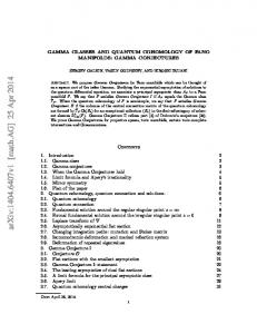
Remark 2.5.6. Applying Watson’s lemma to (2.5.5), we obtain the asymptotic expansion Yτ (z)eU/z ∼ Ψ(id +R1 z + R2 z 2 + · · · ) as z → 0 in the sector | arg z −ϕ| < π2 +ϵ. The right-hand side is called a formal solution which is typically divergent. The existence of a formal solution in the case where u1 , . . . , uN are not distinct was also remarked by Teleman [61, Theorem 8.15]. Our construction shows that each Rk depends analytically on τ , which is not clear from the standard recursive construction of a formal solution. In other words, a semisimple point of a Frobenius manifold is never a turning point. 2.6. Mutation and Stokes matrix. In this section, we discuss mutation of flat sections and Stokes matrices. The braid group action on the irregular monodromy data (Yτ , S) via mutation was discussed by Dubrovin [17, Lecture 4]. We use the idea of Balser-Jurkat-Lutz [5] b and extend expressing Stokes data in terms of monodromy of the Laplace-dual connection ∇ the result of Dubrovin to the case where some of u1 , . . . , uN may coincide. The results here lead us to the formulation of a marked reflection system in §4.2-4.3, §4.5. u1 •

u2 = · · · = ur • ur+1 • uN •

.. .

L1 L2 = · · · = Lr L′1 Lr+1 .. . LN

Figure 1. Right mutation of L1 (where eiϕ = 1 is admissible) Recall that we constructed the asymptotically exponential flat section yi (τ, z) as the Laplace b section yî (τ, λ) over a straight half-line Li = ui + R⩾0 eiϕ . We transform (2.5.5) of the ∇-flat study the change of flat sections under a change of integration paths. To illustrate, we consider the change of paths from L1 to L′1 depicted in Figure 1. In the passage from L1 to L′1 , the path is assumed to cross only one eigenvalue u2 = · · · = ur of multiplicity r − 1. We use the b straight paths L1 , . . . , LN ∪ as branch cuts for ∇-flat sections and regard yî (λ) as a single-valued analytic function on C\ j̸=i Lj . Let M denote the anti-clockwise monodromy transformation b around λ = u2 acting on the space of ∇-flat sections. By Lemma 2.5.3 (2), the monodromy transform of yˆ1 can be written as: M yˆ1 = yˆ1 − c12 yˆ2 − · · · − c1r yˆr for some coefficients c12 , . . . , c1r ∈ C. From this it follows that the flat section y1′ (z) defined by the integral over L′1 is given by: (2.6.1)

y1′ (z) = y1 (z) − c12 y2 (z) − · · · − c1r yr (z).

We call the flat section y1′ (z) (or the path L′1 ) the right mutation of y1 (z) (resp. L1 ) with respect to u2 = · · · = ur . The left mutation of a flat section or a path is the inverse operation: see Figure 2. A mutation occurs when we vary the direction eiϕ and eiϕ becomes non-admissible. We now let the phase ϕ decrease by the angle π continuously. Then the asymptotically exponential − flat sections y1 , . . . , yN undergo a sequence of right mutations. Let y1− , . . . , yN be the basis

14


u1 •

L1 L′r+1 • ur+1

• u2 = · · · = ur

L2 = · · · = Lr Lr+1

Figure 2. Left mutation of Lr+1 of asymptotically exponential flat sections associated to −eiϕ as in Proposition 2.5.1. In the situation of Figure 1, we successively right-mutate L′1 across ur+1 , ur+2 , . . . , uN , arriving at: ( ) linear combinations of yj (z) (2.6.2) y1− (z) = y1 (z) − c12 y2 (z) − · · · − c1r yr (z) − with Im(e−iϕ u ) < Im(e−iϕ . u2 ) j

yi−

In this way we can write as a linear combination of yj ’s and vice versa. The transition matrix is called the Stokes matrix.

Π+ z 9

Y − (z)

• y :

-

Y (z)

ϕ admissible

Π− Figure 3. Domains of the two solutions Y and Y − Definition 2.6.3 ([4, Remark 1.6], [17, Definition 4.3]). Let Y = (y1 , . . . , yN ), Y − = − (y1− , . . . , yN ) be the fundamental solution associated to an admissible direction eiϕ and −eiϕ respectively as in Proposition 2.5.1. Let Π+ ∪ Π− be the domain in Figure 3 where both Y and Y − are defined. The Stokes matrices (or Stokes multipliers) are the constant matrices4 S and S− satisfying Y (z) = Y − (z)S

for z ∈ Π+

Y (z) = Y − (z)S− for z ∈ Π− − ) be the Proposition 2.6.4 ([17, Theorem 4.3, (4.39)]). Let (y1 , . . . , yN ) and (y1− , . . . , yN asymptotically exponential fundamental solution associated to admissible directions eiϕ and −eiϕ respectively and let S = (Sij ), S− = (S−,ij ) be the Stokes matrices. We have (1) Sij = S−,ji = (yi (τ, e−πi z), yj (τ, z))F for z ∈ Π+ . Here we write e−πi z instead of −z to specify the path of analytic continuation. Similarly, (yi− (τ, eπi z), yj− (τ, z))F gives the coefficient (S −1 )ij of the inverse matrix of S. 4Our Stokes matrices are inverse to the ones in [17, Definition 4.3].


15

(2) The Stokes matrix S is a triangular matrix with diagonal entries all equal to one. More precisely, we have Sii = 1 for all i and Sij = 0

if i ̸= j and ui = uj ;

Sij = 0

if Im(e−iϕ ui ) < Im(e−iϕ uj ).

In particular, S, S− do not depend on τ and y1 , . . . , yN are semiorthonormal. Proof. Dubrovin [17] discussed the case where u1 , . . . , uN are distinct. We have yj (z) = ∑N ∑N − − k=1 yk (z)Skj for z ∈ Π+ and yj (z) = k=1 yk (z)S−,kj for z ∈ Π− . Taking the pairing with − yi (−z) and using the property (yk (z), yi (−z))F = δki from Proposition 2.5.1, we obtain (yi (−z), yj (z))F = Sij (yi (−z), yj (z))F = S−,ij

for z ∈ Π+ for z ∈ Π−

Replacing z with −z in the second formula and taking into account the direction of analytic continuation, we see that (1) and (2) hold. (The discussion for (yi− (eπi z), yj− (z))F is similar.) As already discussed, the coefficients of the Stokes matrix arise from a sequence of mutations. Part (3) is obvious from this. □ Remark 2.6.5. We often choose an ordering of normalized idempotents Ψ1 , . . . , ΨN so that the corresponding eigenvalues satisfy Im(e−iϕ u1 ) ⩾ · · · ⩾ Im(e−iϕ uN ). Then the Stokes matrix becomes upper -triangular. Note also that flat sections yi corresponding to the same eigenvalue are mutually orthogonal. Let us go back to the situation of Figure 1. The coefficient c1i appearing in (2.6.2) coincides with the coefficient S1i of the Stokes matrix, because by inverting (2.6.2) we obtain ( ) linear combinations of yj− (z) y1 (z) = y1− (z) + c12 y2− (z) + · · · + c1r yr− (z) + −iϕ −iϕ with Im(e

uj ) < Im(e

u2 )

for z ∈ Π− and therefore c1i = S−,i1 = S1i . Recall that c1i arises as the coefficient of the right mutation (2.6.1). Therefore we obtain the following corollary: Corollary 2.6.6 ([17, Theorem 4.6]). Let eiϕ be an admissible direction and let (y1 , . . . , yN ) be the asymptotically exponential fundamental solution associated to eiϕ in Proposition 2.5.1. Let ua , ub be distinct eigenvalues such that there are no eigenvalues uj with Im(e−iϕ ua ) > Im(e−iϕ uj ) > Im(e−iϕ ub ). Then the right mutation of the flat section ya (z) with respect to ub is given by ∑ ya 7→ ya − Saj yj . j:uj =ub

Similarly, the left mutation of yb (z) with respect to ua is given by: ∑ yb 7→ yb − Sjb yj j:uj =ua

where Sij = (yi (τ, e−πi z), yj (τ, z))F are the coefficients of the Stokes matrix. 2.7. Isomonodromic deformation. In semisimple case, the base of the big quantum connection (2.2.3) can be extended to the universal covering of a configuration space. Suppose that the quantum product is convergent and semisimple in a neighbourhood of q τ = 0 ∈ H (F ). Since the eigenvalues u1 , . . . , uN of E⋆τ form a local co-ordinate system q H (F ), we can make u1 , . . . , uN pairwise distinct by a small deformation of τ . We take a base q point τ ◦ ∈ H (F ) such that the corresponding eigenvalues u◦ = {u◦1 , . . . , u◦N } are pairwise

16


distinct. The quantum connection ∇|τ ◦ then admits a unique isomonodromic deformation over the universal cover CN (C)∼ of the configuration space / (2.7.1) CN (C) = {(u1 , . . . , uN ) ∈ CN : ui ̸= uj for all i ̸= j} SN . Proposition 2.7.2 ([17, Lemma 3.2, Exercise 3.3, Lemma 3.3]). We have a unique meroq morphic flat connection on the trivial H (F )-bundle over CN (C)∼ × P1 of the form: ∂ 1 + Ci ∇ ∂ = ∂ui ∂ui z ∂ 1 ∇z ∂ = z − U +µ ∂z ∂z z q where Ci and U are End(H (F ))-valued holomorphic functions on CN (C)∼ , such that it restricts to the big quantum connection (2.2.3) in a neighbourhood of the base point u◦ . Here the eigenvalues of U give the co-ordinates u1 , . . . , uN on the base. Remark 2.7.3 ([17, Lemma 3.3]). This isomonodromic deformation defines a Frobenius manifold structure on an open dense subset of CN (C)∼ . 3. Gamma Conjecture I In this section we formulate Gamma conjecture I for arbitrary Fano manifolds. We do not need to assume the semisimplicity of the quantum cohomology algebra. 3.1. Property O. We introduce Property O for a Fano manifold F .

q

Definition 3.1.1. Let F be a Fano manifold and let c1 (F )⋆0 ∈ End(H (F )) be the quantum product at τ = 0 (see §2.1). Set T := max{|u| : u is an eigenvalue of (c1 (F )⋆0 )}. We say that F satisfies Property O if (1) T is an eigenvalue of (c1 (F )⋆0 ). (2) If u is an eigenvalue of (c1 (F )⋆0 ) with |u| = T , we have u = T ζ for some r-th root of unity ζ ∈ C, where r is the Fano index of F . (3) The multiplicity of the eigenvalue T is one. Conjecture 3.1.2 (Conjecture O). Every Fano manifold satisfies Property O. The number T ∈ R⩾0 above is an algebraic number. This is an invariant of a monotone symplectic manifold. Conjecture O says that T is non-zero unless F is a point. We do not have a general argument to show Conjecture O, but there are a few weak evidences as follows. Remark 3.1.3. Let r be the Fano index. The formula (2.2.5) shows that we have ⋆0 = ⋆τ with τ = c1 (F )(2πi/r). This together with (2.2.6) gives the symmetry: (3.1.4)

(c1 (F )⋆0 ) = e2πi/r e−2πiµ/r (c1 (F )⋆0 )e2πiµ/r

Therefore the spectrum of (c1 (F )⋆0 ) is invariant under multiplication by e2πi/r . Remark 3.1.5 (O is the structure sheaf). Mirror symmetry for Fano manifolds claims that F is mirror to a holomorphic function f : Y → C on a complex manifold Y . Under mirror symmetry it is expected that the eigenvalues of (c1 (F )⋆0 ) should coincide with the critical values of f . Each Morse critical point of f associates a vanishing cycle (or Lefschetz thimble) which gives an object of the Fukaya-Seidel category of f . Under homological mirror symmetry, the vanishing cycle associated to T should correspond to the structure sheaf O of F . This


17

explains the name ‘Conjecture O’. Our Gamma conjectures give a direct link between T and O in terms of differential equations (without referring to mirror symmetry): the asymptotically bF = Γ b F Ch(O); more generally exponential flat section associated to T should correspond to Γ b F Ch(E) for an exceptional object E ∈ Db (F ) a simple eigenvalue should correspond to Γ coh (see Gamma Conjecture I, II in §3.4, §4.6). Remark 3.1.6 (Conifold point [24]). Let f : (C× )n → C be a convenient5 Laurent polynomial mirror to a Fano manifold F . Suppose that all the coefficients of f are positive real. Then the Hessian ∂2f (x1 , . . . , xn ) ∂ log xi ∂ log xj is positive definite on the subspace (R>0 )n . Thus f |(R>0 )n attains a global minimum at a unique critical point xcon in the domain (R>0 )n ; also the critical point xcon is non-degenerate. We call the point xcon the conifold point. Many examples suggest that T equals Tcon := f (xcon ). Remark 3.1.7 (Perron-Frobenius eigenvalue). This remark is due to Kaoru Ono. We say that a square matrix M of size n is irreducible if the linear map Cn → Cn , v 7→ M v admits no invariant co-ordinate subspace. If (c1 (F )⋆0 ) is represented by an irreducible matrix with nonnegative entries, T is a simple eigenvalue of (c1 (F )⋆0 ) by Perron-Frobenius theorem. Remark 3.1.8 (Fano orbifold). For a Fano orbifold, T may have multiplicity bigger than one. Consider the Z/3Z action on P2 given by [x, y, z] 7→ [x, e2πi/3 y, e4πi/3 z] and let F be the −1 −1 2 2 −1 quotient Fano orbifold P2 /(Z/3Z). The mirror is f = x−1 1 x2 + x1 x2 + x1 x2 and T = 3 has multiplicity three. Under homological mirror symmetry, three critical points in f −1 (T ) correspond to three flat line bundles which are mutually orthogonal in the derived category. One could guess that the multiplicity of T equals the number of irreducible representations of π1orb (F ) for a Fano orbifold F . Remark 3.1.9. In the rest of the section we assume that our Fano manifold F satisfies Property O. However, the argument in this section (i.e. §3) except for §3.7 works under the following weaker assumption: there exists a complex number T such that (1) T is an eigenvalue of (c1 (F )⋆0 ) of multiplicity one and (2) if T˜ is an eigenvalue of (c1 (F )⋆0 ) with Re(T˜) ⩾ Re(T ), then T˜ = T . In §3.7, we use the condition part (2) in Definition 3.1.1. When F satisfies Property O, we write (3.1.10)

T ′ := max {Re(u) : u ̸= T, u is an eigenvalue of (c1 (F )⋆0 )} < T

for the second biggest real part for the eigenvalues of (c1 (F )⋆0 ). 3.2. Asymptotic solutions along positive real line. We construct a fundamental solution for ∇ with nice asymptotic properties over the positive real line; here we do not assume semisimplicity, cf. §2.5. Suppose that a Fano manifold F satisfies Property O. Let λ1 , . . . , λk be the distinct eigenvalues of (c1 (F )⋆0 ) and let Ni be the multiplicity of λi . Note that N = N1 + · · · + Nk . We may assume that T = λ1 ; Property O implies N1 = 1. Note that the Euler vector field 5A Laurent polynomial is said to be convenient if the Newton polytope of f contains the origin in its interior.

18


E at τ = 0 equals c1 (F ). We may also (E⋆τ )|τ =0 = (c1 (F )⋆0 ) is of the form:  u1  u2  U = ..  .

assume that the matrix U (2.4.1) of eigenvalues of 

 T     =  

    

λ2 IN2 ..

.

uN

λk INk q

where INi is the identity matrix of size Ni . Choose a linear isomorphism Ψ : CN → H (F ) which transforms (c1 (F )⋆0 ) to the block-diagonal form:   B1   B2   Ψ−1 (c1 (F )⋆0 )Ψ =   . .   . Bk where Bi is a matrix of size Ni and Bi − λi INi is nilpotent. Proposition 3.2.1. Suppose that a Fano manifold F satisfies Property O. With the notation as above, there exists a fundamental matrix solution for the quantum connection ∇z∂z (2.2.1) at τ = 0 of the form   F1 (z)   F2 (z)   P (z)e−U/z   . .   . Fk (z) over a sufficiently small sector S = {z ∈ C× : |z| ⩽ 1, | arg(z)| ⩽ ϵ} with ϵ > 0 such that (1) P (z) has an asymptotic expansion P (z) ∼ Ψ + P1 z + P2 z 2 + · · · as z → 0 in S; (2) Fi (z) is a GLNi (C)-valued function satisfying the estimate max(∥Fi (z)∥, ∥Fi (z)−1 ∥) ⩽ C exp(δ|z|−p ) on S for some C, δ > 0 and 0 < p < 1. (3) F1 (z) = 1. Proof. By a result of Sibuya [58] and Wasow [65, Theorem 12.2], we can find a gauge transformation P (z) over S satisfying (1) above such that the new connection matrix C(z) P (z)−1 ∇∂z P (z) = ∂z − z −2 C(z) satisfies: • C(z) = diag[C1 (z), . . . , Ck (z)] is block-diagonal with Ci (z) being of size Ni ; • Ci (z) has an asymptotic expansion Ci (z) ∼ Ci,0 + Ci,1 z + Ci,2 z 2 + · · · as z → 0 in S; • Ci,0 − λi INi is nilpotent. Now it suffices to find a fundamental solution for the ith block ∇(i) := ∂z −z −2 Ci (z). We have eλi /z ∇(i) e−λi /z = ∂z − z −2 (Ci (z) − λi INi ) and the leading term of the asymptotic expansion of Ci (z) − λi INi is nilpotent. By [59, Lemma 5.4.1], any fundamental solution Fi (z) for ∂z − z −2 (Ci (z) − λi INi ) satisfies the estimate in part (2) for 1 − 1/Ni < p < 1. We show that part (3) can be achieved. Set D(z) = C1 (z) − λ1 . Then F1 (z) is a solution to the scalar differential equation (∂z − z −2 D(z))F1 (z) = 0. Arguing as in [65, Theorem 12.3], we find that F1 (z) = z c g(z) for some c ∈ C and a holomorphic function g(z) on S which has an asymptotic expansion g(z) ∼ a0 + a1 z + a2 z 2 + · · · at z = 0 with a0 ̸= 0. Thus we obtain


19

a ∇-flat section s1 (z) = e−T /z z c g(z)P1 (z) where P1 (z) is the first column of P (z). Studying the asymptotics of the equation ∇s1 (z) = 0 (using e.g. [65, Theorem 8.8]), we have (µ + c)a0 P1 (0) ∈ Im((c1 (F )⋆0 ) − T ). Recall that P1 (0) is a non-zero T -eigenvector of (c1 (F )⋆0 ). By Lemma 3.2.2 below, we must have c = 0. Thus we can absorb F1 (z) = g(z) into the first column of P (z). □ q

Lemma 3.2.2. Suppose that a Fano manifold F satisfies Property O. Let E(T ) ⊂ H (F ) denote the one-dimensional T -eigenspace of (c1 (F )⋆0 ) and define H ′ := Im(T − (c1 (F )⋆0 )) which is a complementary subspace of E(T ). Then E(T ) and H ′ are orthogonal with respect to the Poincaré pairing and the endomorphism µ satisfies µ(E(T )) ⊂ H ′ . q

Proof. Take α ∈ E(T ) and β ∈ H ′ . There exists an element γ ∈ H (F ) such that β = (T − c1 (F )⋆0 )γ. Then we have (α, β)F = (α, T γ − c1 (F ) ⋆0 γ)F = (T α − c1 (F ) ⋆0 α, γ)F = 0. Thus E(T ) ⊥ H ′ with respect to (·, ·)F . The skew-adjointness of µ with respect to (·, ·)F shows that (µα, α)F = 0; hence µ(α) ∈ H ′ . □ 3.3. Flat sections with the smallest asymptotics. Under Property O, one can find a one-dimensional vector space A of flat sections s(z) having the most rapid exponential decay s(z) ∼ e−T /z as z → +0 on the positive real line. We refer to such sections as flat sections with the smallest asymptotics. It is easy to deduce the following result from Proposition 3.2.1. Proposition 3.3.1. Suppose that a Fano manifold F satisfies Property O. Consider the quantum connection ∇ in (2.2.1) and define: { } q T /z −m A := s : R>0 → H (F ) : ∇s = 0, ∥e s(z)∥ = O(z ) as z → +0 (∃m) (3.3.2) Then: (1) A is a one-dimensional complex vector space. (2) For s ∈ A, the limit limz→+0 eT /z s(z) exists and lies in the T -eigenspace E(T ) of (c1 (F )⋆0 ). The map A → E(T ) defined by this limit is an isomorphism. q (3) Let s : R>0 → H (F ) be a flat section which does not belong to A. Then we have limz→+0 ∥eλ/z s(z)∥ = ∞ for all λ > T ′ where T ′ is in (3.1.10). 3.4. Gamma Conjecture I: statement. The Gamma class [51, 52, 44, 49, 45] of a smooth projective variety F is the class b F := Γ

dim ∏F

q

Γ(1 + δi ) ∈ H (F )

i=1

where δ1 , . . . , δdim F are the Chern roots of the tangent bundle T F so that ∏ F c(T F ) = dim i=1 (1 + δi ). The Gamma function Γ(1 + δi ) in the right-hand side should be expanded in the Taylor series in δi . We have ( ) ∞ ∑ k b F = exp −Ceu c1 (F ) + Γ (−1) (k − 1)!ζ(k) chk (T F ) k=2

where Ceu = 0.57721... is Euler’s constant and ζ(k) is the special value of Riemann’s zeta function.

20


The fundamental solution S(z)z −µ z ρ from Proposition 2.3.1 identifies the space of flat sections over the positive real line R>0 with the cohomology group: q

q

Φ : H (F ) −→ {s : R>0 → H (F ) : ∇s = 0}

(3.4.1)

α 7−→ (2π)−

dim F 2

S(z)z −µ z ρ α

where we use the standard determination for z −µ z ρ = exp(−µ log z) exp(ρ log z) such that log z ∈ R for z ∈ R>0 . Definition 3.4.2. Suppose that a Fano manifold F satisfies Property O. The principal q asymptotic class of F is a cohomology class AF ∈ H (F ) such that A = CΦ(AF ), where A is the space (3.3.2) of flat sections with the smallest asymptotics (recall that A is of dimension one by Proposition 3.3.1). The class AF is defined up to a constant; when ⟨[pt], AF ⟩ ̸= 0, we can normalize AF so that ⟨[pt], AF ⟩ = 1. Conjecture 3.4.3 (Gamma Conjecture I). Let F be a Fano manifold F satisfying Property bF . O. The principal asymptotic class AF of F is given by Γ We explain that the Gamma class should be viewed as a square root of the Todd class (or b A-class) in the Riemann-Roch theorem. Let H denote the vector space of ∇-flat sections over the positive real line: q H := {s : R>0 → H (F ) : ∇s = 0} and let [·, ·) be a non-symmetric pairing on H defined by [s1 , s2 ) := (s1 (e−iπ z), s2 (z))F

(3.4.4)

for s1 , s2 ∈ H, where s1 (e−iπ z) denotes the analytic continuation of s1 (z) along the semicircle [0, 1] ∋ θ 7→ e−iπθ z. The right-hand side does not depend on z because of the flatness (2.2.2). q The non-symmetric pairing [·, ·) induces a pairing on H (F ) via the map Φ (3.4.1); we denote q by the same symbol [·, ·) the corresponding pairing on H (F ). Since S(z) preserves the pairing (Proposition 2.3.1), we have 1 1 (3.4.5) [α, β) = (eπiµ e−πiρ α, β)F = (eπiρ eπiµ α, β)F dim F (2π) (2π)dim F q

for α, β ∈ H (F ). We write Ch(·), Td(·) for the following characteristic classes: Ch(V ) = (2πi)

deg 2

ch(V ) =

rank ∑V

e2πiδj

j=1

Td(V ) = (2πi)

deg 2

td(V ) =

rank ∏V j=1

2πiδj 1 − e−2πiδj

where δ1 , . . . , δrank V are the Chern roots of a vector bundle V . We also write TdF = Td(T F ). Lemma 3.4.6 ([44, 45]). Let V1 , V2 be vector bundles over F . Then [ ) b F Ch(V1 ), Γ b F Ch(V2 ) = χ(V1 , V2 ) Γ ∑ F i i where χ(V1 , V2 ) = dim i=0 (−1) dim Ext (V1 , V2 ). Proof. Recall the Gamma function identity: (3.4.7)

Γ(1 + z)Γ(1 − z) =

2πiz . − e−iπz

eiπz


This immediately implies that

Therefore

[

21

( deg ) b F = TdF . bF · Γ eπiρ eπi 2 Γ

) b F Ch(V1 ), Γ b F Ch(V2 ) = Γ

1 (2πi)dim F

∫ (

eπi

deg 2

) Ch(V1 ) Ch(V2 ) TdF .

F

This equals χ(V1 , V2 ) by the Hirzebruch-Riemann-Roch formula.

□

b F ) of A satisfies the following Under Gamma Conjecture I, the canonical generator Φ(Γ normalization. Proposition 3.4.8. Suppose that a Fano manifold F satisfies Property O and Gamma Conb F )(z). Then we have: jecture I. Set s1 (z) = Φ(Γ (1) The limit v := limz→+0 eT /z s1 (z) ∈ E(T ) satisfies (v, v)F = 1. b ∂ be the Laplace dual (2.5.2) of the quantum connection ∇ at τ = 0. There (2) Let ∇ λ b ∂ -flat section φ(λ) which is holomorphic near λ = T such that φ(T ) = v exists a ∇ λ ∫∞ and that s1 (z) = z −1 T φ(λ)e−λ/z dλ. Proof. We give a construction of the generator s1 of A using Laplace transformation as in b §2.5. Recall that once we have a ∇-flat section φ(λ) holomorphic near λ = T such that φ(T ) is a non-zero eigenvector v of (c1 (F )⋆0 ) with eigenvalue T , the Laplace transform ∫ 1 ∞ s1 (z) = φ(λ)e−λ/z dλ z T gives a ∇-flat section such that limz→+0 eT /z s1 (z) = v (see the discussion around (2.5.5)). b b Thus it suffices to construct a ∇-flat section φ(λ) as above. Property O ensures that ∇ b at λ = T is is logarithmic at λ = T , and Lemma 3.2.2 ensures that the residue R of ∇ b of the form nilpotent and Rv = 0. Thus we have a fundamental matrix solution for ∇ U (λ) exp(−R log(λ − T )) with U (λ) holomorphic near λ = T and U (T ) = id [65, Theorem b 5.5]. Now φ(λ) := U (λ) exp(−R log(λ − T ))v = U (λ)v gives the desired ∇-flat section. It now suffices to show that v = φ(T ) is of unit length. By bending the integration path [T, ∞] as in Figure 4, we obtain the analytic continuation s1 (e−πi z) of s1 (z). Watson’s lemma [1, §6.2.2] shows that limz→+0 e−T /z s1 (e−πi z) = v. Therefore we have [ ) ( ) bF , Γ b F = Φ(Γ b F )(e−πi z), Φ(Γ b F )(z) Γ = (s1 (e−πi z), s1 (z))F → (v, v)F F

as z → +0. By Lemma 3.4.6, the left-hand side equals χ(OF , OF ) = 1 since F is Fano. Thus we have (v, v)F = 1 and the conclusion follows. □ 3.5. The leading asymptotics of dual flat sections. We now study flat sections of the dual quantum connection, which we call dual flat sections. We show that the limit limz→+0 eT /z f (z) exists for every dual flat section f (z). Let H q (F ) = Heven (F ; C) denote the even part of the homology group with complex coefficients. The dual quantum connection is a meromorphic flat connection on the trivial bundle H q (F ) × P1 → P1 given by (cf. (2.2.1)) (3.5.1)

=z ∇∨ z ∂ ∂z

∂ 1 + (c1 (F )⋆0 )t − µt ∂z z

22


• • • b F )(e−πi z) Φ(Γ

•

• •

b )(z) Φ(Γ - F

T

•

Figure 4. Spectrum of (c1 (F )⋆0 ) and the paths of integration (on the λ-plane). where the superscript “t” denotes the transpose. This is dual to the quantum connection ∇ in the sense that we have d⟨f (z), s(z)⟩ = ⟨∇∨ f (z), s(z)⟩ + ⟨f (z), ∇s(z)⟩ where ⟨·, ·⟩ is the natural pairing between homology and cohomology. Because of the property (2.2.2), we can identify the dual flat connection ∇∨ with the quantum connection ∇ with the opposite sign of z. In order to avoid possible confusion about signs, we shall not use this identification. We write E(T )∗ ⊂ H q (F ) for the one-dimensional eigenspace of (c1 (F )⋆0 )t with eigenvalue T and H ′ ∗ := Im(T − (c1 (F )⋆0 )t ) for a complementary subspace. They are dual to E(T ), H ′ from Lemma 3.2.2. Proposition 3.5.2. Suppose that a Fano manifold F satisfies Property O. Then: (1) The limit Lead(f ) := lim e−T /z f (z) z→+0

∇∨ -flat

exists for every a linear functional: Lead :

section f (z) and lies in E(T )∗ . In other words, Lead defines

{ } f : R>0 → H q (F ) : ∇∨ f (z) = 0 −→ E(T )∗ .

(2) If Lead(f ) = 0, we have limz→+0 e−λ/z f (z) = 0 for every λ > T ′ . Proof. Note that a fundamental solution for ∇∨ is given by the inverse transpose of that for ∇. The conclusion follows easily by using the fundamental solution in Proposition 3.2.1. □ 3.6. A limit formula for the principal asymptotic class. The leading asymptotic behaviour of dual flat sections as z → +0 is given by the pairing with a flat section with the smallest asymptotics. From this we obtain a limit formula for AF . The fundamental solution for the dual quantum connection ∇∨ (3.5.1) is given by the inverse transpose (S(z)z −µ z ρ )−t of the fundamental solution for ∇ in Proposition 2.3.1. This yields the following identification (cf. (3.4.1)) (3.6.1)

Φ∨ : H q (F ) −→ {f : R>0 → H q (F ) : ∇∨ f (z) = 0} α 7−→ (2π)

dim F 2

S(z)−t z µ z −ρ α t

between dual flat sections and homology classes. 1

t


23

Proposition 3.6.2. Suppose that F satisfies Property O. Let AF be a principal asymptotic class (Definition 3.4.2). Let ψ0∗ be an element of E(T )∗ which is dual to ψ0 := limz→+0 eT /z Φ(AF )(z) ∈ E(T ) in the sense that ⟨ψ0∗ , ψ0 ⟩ = 1. Then we have: Lead(Φ∨ (α)) := lim e−T /z Φ∨ (α)(z) = ⟨α, AF ⟩ψ0∗ . z→+0

Proof. By the definition of Φ and

Φ∨

(see (3.4.1), (3.6.1)), we have:

⟨α, AF ⟩ = ⟨Φ∨ (α)(z), Φ(AF )(z)⟩ = ⟨e−T /z Φ∨ (α)(z), eT /z Φ(AF )(z)⟩. This converges to ⟨Lead(Φ∨ (α)), ψ0 ⟩ as z → +0 by Propositions 3.3.1, 3.5.2.

□

Definition 3.6.3 ([29]). Let S(z)z −µ z ρ be the fundamental solution from Proposition 2.3.1 and set t := z −1 . The J-function J(t) of F is a cohomology-valued function defined by: q

J(t) := z

dim F 2

z −ρ z µ S(z)−1 1

where 1 ∈ H (F ) is the identity class. Alternatively we can define J(t) by the requirement that ( z ) dim F 2 (3.6.4) ⟨α, J(t)⟩ = ⟨Φ∨ (α)(z), 1⟩ 2π holds for all α ∈ H q (F ), using the dual flat sections Φ∨ (α) in (3.6.1). Remark 3.6.5. The J-function is a solution to the scalar differential equation associated to the quantum connection on the anticanonical line τ = c1 (F ) log t. More precisely, we have ) ( ∂) ( J(t) = 0 P t, [∇c1 (F ) ]z=1 1 = 0 ⇐⇒ P t, t ∂t ∂ ∂ for any differential operators P ∈ C⟨t, t ∂t ⟩, where [∇c1 (F ) ]z=1 = t ∂t + (c1 (F )⋆c1 (F ) log t ). Differential equations satisfied by the J-function are called the quantum differential equations. See also Remark 2.2.4.

Remark 3.6.6. Using the fact that S(z)−1 equals the adjoint of S(−z) (Proposition 2.3.1) and Remark 2.3.2, we have   ⟨ ⟩F N ∑ ∑ ϕi (3.6.7) J(t) = ec1 (F ) log t 1 + tc1 (F )·d ϕi  1 − ψ 0,1,d i=1 d∈Eff(F )\{0}

q

i N where {ϕi }N e i=1 and {ϕ }i=1 are bases of H (F ) which are dual with respect to the Poincar´ pairing (·, ·)F . This gives a well-known form of Givental’s J-function [29] restricted to the anticanonical line τ = c1 (F ) log t.

Theorem 3.6.8. Suppose that a Fano manifold F satisfies Property O. Let AF be a principal asymptotic class (Definition 3.4.2) and let J(t) be the J-function. We have J(t) AF = t→+∞ ⟨[pt], J(t)⟩ ⟨[pt], AF ⟩ lim

where the limit is taken over the positive real line and exists if and only if ⟨[pt], AF ⟩ ̸= 0. Proof. By Proposition 3.6.2, we have lim e−T /z Φ∨ (α)(z) = ⟨α, AF ⟩ψ0∗

z→+0

lim e−T /z Φ∨ ([pt])(z) = ⟨[pt], AF ⟩ψ0∗

z→+0

24


for some non-zero ψ0∗ ∈ E(T )∗ . Therefore by (3.6.4) we have ⟨α, J(t)⟩ e−T /z ⟨Φ∨ (α)(z), 1⟩ ⟨α, AF ⟩ = lim −T /z ∨ = t→+∞ ⟨[pt], J(t)⟩ z→+0 e ⟨[pt], AF ⟩ ⟨Φ ([pt])(z), 1⟩ lim

for all α ∈ H q (F ). Here we used the fact ⟨ψ0∗ , 1⟩ ̸= 0 which is proved in Lemma 3.6.10 below. The limit exists if and only if ⟨[pt], AF ⟩ ̸= 0. The Theorem is proved. □ Corollary 3.6.9. Suppose that a Fano manifold F satisfies Property O. The following statements are equivalent: (1) Gamma Conjecture I (Conjecture 3.4.3) holds for F . b F )(z)∥ ⩽ Ce−λ/z on (0, 1] for some C > 0 and λ > T ′ , where T ′ is given in (2) ∥Φ(Γ (3.1.10) and Φ is given in (3.4.1). (3) We have J(t) bF lim =Γ t→+∞ ⟨[pt], J(t)⟩ where J(t) is the J-function of F given in Definition 3.6.3 and the limit is taken over the positive real line. Proof. The equivalence of (1) and (2) is clear from Proposition 3.3.1. The equivalence of (1) and (3) follows from Theorem 3.6.8. □ Lemma 3.6.10. Suppose that F satisfies Property O. For a non-zero eigenvector ψ0∗ ∈ E(T )∗ , we have ⟨ψ0∗ , 1⟩ ̸= 0. In other words, the E(T )-component of 1 with respect to the q decomposition H (F ) = E(T ) ⊕ H ′ in Lemma 3.2.2 does not vanish. Proof. Let ψ0 ∈ E(T ) be a non-zero eigenvector of (c1 (F )⋆0 ) with eigenvalue T . We claim that ψ0 ⋆0 H ′ = 0. Take α ∈ H ′ and write α = T γ − c1 (F ) ⋆0 γ. Then we have ψ0 ⋆ α = T ψ0 ⋆0 γ − ψ0 ⋆0 c1 (F ) ⋆0 γ = 0. The claim follows. Write 1 = cψ0 + ψ ′ with ψ ′ ∈ H ′ and c ∈ C. Applying (ψ0 ⋆0 ), we obtain ψ0 = cψ0 ⋆0 ψ0 . Thus c ̸= 0 and Lemma follows. □ Remark 3.6.11. See [15, §7] for a discussion of the limit formula in the classification problem of Fano manifolds. 3.7. Apery limit. We can replace the continuous limit of the ratio of the J-function appearing in Theorem 3.6.8 with the (discrete) limit of the ratio of the Taylor coefficients. Golyshev [31] considered such limits and called them Apery constants of Fano manifolds. A generalization to Apery class was studied by Galkin [23]. This limit sees the primitive part of the Gamma class. Expand the J-function as ∑ J(t) = ec1 (F ) log t Jn tn . n⩾0

q

The coefficient Jn ∈ H (F ) is given by: Jn :=

N ∑

∑

i=1 d∈Eff(F ):c1 (F )·d=n

⟨ ⟩F ϕi ψ n−2−dim ϕi

0,1,d

ϕi

where we set dim ϕi = dim F − 12 deg ϕi . See Remark 3.6.6. The main theorem in this section is stated as follows:


25

Theorem 3.7.1. Suppose that F satisfies Property O and suppose also that the principal asymptotic class AF satisfies ⟨[pt], AF ⟩ ̸= 0. Let r be the Fano index. For every α ∈ H q (F ) such that c1 (F ) ∩ α = 0, we have ⟨α, Jrn ⟩ ⟨α, A ⟩ F = 0. lim inf − n→∞ ⟨[pt], Jrn ⟩ ⟨[pt], AF ⟩ Remark 3.7.2. Note that Jn = 0 unless r divides n. In the left-hand side of the above formula, we set ⟨α, Jrn ⟩/⟨[pt], Jrn ⟩ = ∞ if ⟨[pt], Jrn ⟩ = 0. It is however expected that the following properties will hold for Fano manifolds: • the Gromov–Witten invariants ⟨[pt], Jrn ⟩ are all positive for n ⩾ 0; • lim inf n→∞ in Theorem 3.7.1 can be replaced with limn→∞ . Remark 3.7.3. More generally, if α, β ∈ H q (F ) are homology classes such that α ∩ c1 (F ) = β ∩ c1 (F ) = 0 and if we have ⟨β, AF ⟩ ̸= 0, we have the limit formula ⟨α, Jrn ⟩ ⟨α, AF ⟩ = 0. lim inf − n→∞ ⟨β, Jrn ⟩ ⟨β, AF ⟩ This can be shown by the same argument as below. We shall restrict to the case β = [pt] as Gamma Conjecture I implies ⟨[pt], AF ⟩ ̸= 0. b as: Define the functions G and G G(t) := ⟨[pt], J(t)⟩ =

∞ ∑

Gn tn ,

where Gn := ⟨[pt], Jn ⟩,

n=0

b G(κ) :=

∞ ∑ n=0

1 n!Gn κ = κ

∫

n

∞

G(t)e−t/κ dt.

0

b are called (unregularized or regularized) quantum periods of Fano manThese functions G, G ifolds [15]. b Lemma 3.7.4. Let F be an arbitrary Fano manifold. The convergence radius of G(κ) is bigger than or equal to 1/T . Proof. Recall that we have G(t) = (2πt)− dim F/2 ⟨Φ∨ ([pt])(z), 1⟩ (see (3.6.4)) and Φ∨ ([pt])(z) is a ∇∨ -flat section (where z = t−1 ). By Proposition 3.5.2, we have an estimate ∥Φ([pt])(t−1 )∥ ⩽ C0 eT t on t ∈ [1, ∞) for some constant C0 > 0, and thus the following Laplace transformation converges for λ with Re(λ) < −T and ν ≫ 0, ν ∈ / Z. ∫ ∞ dim F φ(λ) = (2π)− 2 tν−1 eλt Φ∨ ([pt])(t−1 )dt 0

The condition ν ≫ 0 ensures that the integral converges near t = 0 (since ∇∨ is regular singular at t = 0, f (t−1 ) is of at most polynomial growth near t = 0). By the standard e (ν) argument using integration by parts, we can show that φ(λ) is flat for the connection ∇ given by e (ν) = ∂λ + (λ + (c1 (F )⋆0 )t )−1 (−µt + ν). ∇ ∂λ

26


Then the convergence radius of ⟨φ(−κ−1 ), 1⟩ =

∫

∞

tν+

dim F 2

0

(3.7.5)

= κν+

dim F 2

−1

−1

∞ ∑

G(t)e−t/κ dt Γ(n + ν +

n dim F 2 )Gn κ

n=0

e (ν) ∇

b is bigger than or equal to 1/T as has no singularities in {|λ| > T }. The function G(κ) −1 has the same radius of convergence as ⟨φ(−κ ), 1⟩ and the conclusion follows. □ Lemma 3.7.6. Suppose that F satisfies Property O and ⟨[pt], AF ⟩ ̸= 0. Then the convergence b radius of G(κ) is exactly 1/T . Proof. In view of the discussion in the previous lemma, it suffices to show that the function ⟨φ(−κ−1 ), 1⟩ in (3.7.5) has a singularity at κ = 1/T . By (3.6.4) we have G(t) = (2πt)− dim F/2 ⟨Φ∨ ([pt])(z), 1⟩. Thus by Proposition 3.6.2 and Lemma 3.6.10, we have lim e−tT (2πt)

dim F 2

t→+∞

G(t) = ⟨[pt], AF ⟩⟨ψ0∗ , 1⟩ ̸= 0.

Therefore the Laplace transform (3.7.5) diverges as κ approaches 1/T from the left for ν ≫ 0. □ ⟨α,AF ⟩ [pt]. Then ⟨β, AF ⟩ = 0. It suffices to show that Proof of Theorem 3.7.1. Set β := α − ⟨[pt],A F⟩ ⟨β, Jrn ⟩ = 0. (3.7.7) lim inf n→∞ ⟨[pt], Jrn ⟩ ∑ n − dim F/2 ⟨Φ∨ (β)(t−1 ), 1⟩ by Set bn := ⟨β, Jn ⟩. Then we have ∞ n=0 bn t = ⟨β, J(t)⟩ = (2πt) ∨ ∗ (3.6.4). By Proposition 3.6.2, we have Lead(Φ (β)) = ⟨β, AF ⟩ψ0 = 0. Thus by Proposition 3.5.2 we have limt→+∞ e−tλ Φ∨ (β)(t−1 ) = 0 for every λ > T ′ . Consider again the Laplace transform ∫ ∞ dim F tν−1 etλ Φ∨ (β)(t−1 )dt φβ (λ) = (2π)− 2 0

e (ν) -flat section which is regular on for ν ≫ 0 (as in the proof of Lemma 3.7.4). This is a ∇ ′ {λ : Re(λ) < −T }. Then its component ⟨φβ (−κ

−1

F ν+ dim −1 2

), 1⟩ = κ

∞ ∑

Γ(n + ν +

n dim F 2 )bn κ

n=0

has the radius of convergence strictly bigger than 1/T . This is because the only singularities of e (ν) on {|λ| ⩾ T } are {−e2πik/r T : k = 0, . . . , r − 1} and ⟨φβ (λ), 1⟩ is regular at λ = −T and ∇ dim F satisfies ⟨φβ (e2πi/r λ), 1⟩ = e−(ν+ 2 −1)2πi/r ⟨φβ (λ), 1⟩. (Here we used Part (2) of Property O.) This implies that there exist numbers C, R > 0 such that R > 1/T and |bn n!| ⩽ CR−n . On the other hand, Lemma 3.7.6 implies that lim sup |Gn n!|1/n = T. n→∞

Let ϵ > 0 be such that (1 − ϵ)RT > 1. Then we have a number n0 such that for every n ⩾ n0 we have supm⩾n |Gm m!|1/m ⩾ T (1 − ϵ/2). Namely we can find a sequence n0 ⩽ n1 < n2
j. This implies that G is non-degenerate, hence vectors vi are linearly independent so N ⩽ dim V . We say that V is a semiorthonormal basis (SOB) if N = dim V i.e. vi form a basis of vector space V , this implies that pairing [·, ·) is non-degenerate. Set of SOBs admits an obvious action of (Z/2Z)N : if v1 , . . . , vN is SOB then so is ±v1 , . . . , ±vN , in this case we say that SOBs are the same up to sign. For u, v ∈ V , define the right mutation Ru v and the left mutation Lu v by Ru v := v − [v, u)u,

Lu v := v − [u, v)u.

The braid group BN on N strands acts on the set of SOBs of N vectors by: σi (v1 , . . . , vN ) = (v1 , . . . , vi−1 , vi+1 , Rvi+1 vi , vi+2 , . . . , vN ) (4.1.1) −1 σi (v1 , . . . , vN ) = (v1 , . . . , vi−1 , Lvi vi+1 , vi , vi+2 , . . . , vN ) 6The central charge Z(V ) here is denoted by (2πi)dim F Z(V ) in [45].

28


where σ1 , . . . , σN −1 are generators of BN and satisfy the braid relation σi σi+1 σi = σi+1 σi σi+1 σi σj = σj σi

if |i − j| ⩾ 2.

4.2. Marked reflection system. A marked reflection system (MRS) of phase ϕ ∈ R is a tuple (V, [·, ·), {v1 , . . . , vN }, m, eiϕ ) consisting of • a complex vector space V ; • a bilinear form [·, ·) on V ; • an unordered basis {v1 , . . . , vN } of V ; • a marking m : {v1 , . . . , vN } → C; we write ui = m(vi ) and u = {u1 , . . . , uN }; • eiϕ ∈ S 1 ; ϕ ∈ R is called a phase such that the vectors vi are semiorthonormal in the sense that: { 1 if i = j; (4.2.1) [vi , vj ) = 0 if i ̸= j and Im(e−iϕ ui ) ⩽ Im(e−iϕ uj ). When the basis is ordered appropriately, (V, [·, ·), v1 , . . . , vN ) gives an SOB. We say that ϕ ∈ R (or eiϕ ∈ S 1 ) is admissible for a multiset u = {u1 , . . . , uN } in C if eiϕ is not parallel to any non-zero difference ui − uj . An MRS is said to be admissible if the phase ϕ is admissible for u. The circle S 1 acts on the space of all MRSs by rotating simultaneously the phase and all markings: ϕ 7→ α + ϕ, ui 7→ eiα ui . We write hϕ : C → R for the R-linear function hϕ (z) = Im(e−iϕ z). Remark 4.2.2 ([30]). The data of admissible marked reflection system may be used to produce a polarized local system (i.e. a local system with a monodromy-invariant bilinear form) on C \ u: by identifying the fiber with V , endowing it with a bilinear form {·, ·} (either with the symmetric form {v1 , v2 } = [v1 , v2 ) + [v2 , v1 ) or with the skew-symmetric form {v1 , v2 } = [v1 , v2 ) − [v2 , v1 )), choosing “eiϕ ∞” for the base point, joining it with the points ui with the level rays ui + R⩾0 eiϕ as paths, trivializing the local system outside the union of the paths, and requiring that the turn around ui act in the monodromy representation by the reflection with respect to vi : rvi (v) = v − {v, vi }vi . In case ui is a multiple marking all the respective reflections commute, so the monodromy of the local system is well-defined as a product of such reflections. The form {·, ·} could be degenerate, however construction above also provides local systems with fiber the quotient-space V / Ker{·, ·} (use reflections with respect to images of vi in the quotient-spaces). When u1 , . . . , uN are pairwise distinct, this construction could be reversed with a little ambiguity: if there is such a local system and the paths are given, we take V to be a fiber, define vi ∈ V as a reflection vector of the monodromy at ui (which could be determined up to sign if {·, ·} is non-degenerate), and define [vi , vi ) = 1 for all i, for i ̸= j put [vi , vj ) = 0 if hϕ (ui ) < hϕ (uj ) and [vi , vj ) = {vi , vj } otherwise. 4.3. Mutation of MRSs. In this section, we explain how an MRS changes by mutation as we vary the marking u and the phase ϕ. First we give an intuitive explanation and then give a formal definition. The mutation of MRSs is parallel to the mutation of asymptotically exponential flat sections in §2.6 (see Corollary 2.6.6). For a given admissible MRS (V, [·, ·), {v1 , . . . , vN }, m(vi ) = ui , eiϕ ), we draw the ray Li = ui + R⩾0 eiϕ from each marking ui in the direction of ϕ to get a picture as in Figure 5. We consider a variation of the parameters u and ϕ. We allow that a multiple marking separates into distinct ones, but do not allow that two different markings


29

ui ̸= uj collide unless the corresponding vectors vi , vj are orthogonal [vi , vj ) = [vj , vi ) = 0. The vectors v1 , . . . , vN stay constant while each uj does not hit any other rays Li with uj ̸= ui . When uj crosses a ray Li from the right side of Li (resp. the left side of Li ) towards the direction ϕ, the vectors marked by ui undergo the right (resp. left) mutation. In the situation of Figure 6, if a vector vl is marked by ui , it is transformed to   ∏ ∑ [vl , vk )vk vl′ =  Rvk  vl = vl − k:uj =uk

k:uj =uk

after the move. The vectors that are not assigned the marking ui remain the same. Note that the vectors with the same marking uj are orthogonal to each other and hence the above product of Rvk does not depend on the order. Note also that the vectors vl′ marked by ui are mutually orthogonal even after the mutation. u1 •

L1 L2 L3 = L4 = L5 L6 = L7 L8 L9

u2 •

u3 = u4 = u5 • u6 = u7 • u8 • u9 •

Figure 5. Rays Li in the admissible direction eiϕ = 1.

ui •

6

phase ϕ

uj • Figure 6. Right mutation Remark 4.3.1. Let (V, [·, ·), {v1 , . . . , vN }, m(vi ) = ui , eiϕ ) be an admissible MRS with multiple markings. Since we have [vi , vj ) = [vj , vi ) = 0 if ui = uj and i ̸= j (see (4.2.1)), there exists ϵ > 0 such that all the admissible MRSs of the form (V, [·, ·), {v1 , . . . , vN }, m(vi ) = u′i , eiϕ ) with pairwise distinct u′1 , . . . , u′N and |ui − u′i | < ϵ are related to each other by mutation. Now we give a formal and precise definition for the deformation of MRSs. We first deal with the case where u = (u1 , . . . , uN ) are pairwise distinct, i.e. give an element of the configuration space CN (C) (2.7.1). We construct a local system L = L(V, [·, ·)) of MRSs with fixed (V, [·, ·)) over CN (C) × S 1 . Then we extend the étalé space (sheaf space) of L to a branched cover M over S N (C)×S 1 (where S N (C) is the symmetric power of C); this amounts to pushing forward L to S N (C) × S 1 as an orbi-sheaf. We will see that the fiber M(u,eiϕ ) at (u, eiϕ ) ∈ S N (C) × S 1 contains the set of all MRSs on (V, [·, ·)) with marking u and phase ϕ. Then we define a deformation of MRSs as a continuous path in M.

30


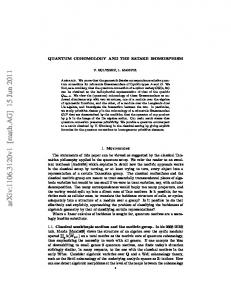
Local system on the ‘distinct’ locus. Consider the codimension-one stratum W ⊂ CN (C) × S 1 consisting of non-admissible parameters (u, eiϕ ): W = {(u, eiϕ ) ∈ CN (C) × S 1 : hϕ (ui ) = hϕ (uj ) for some i ̸= j}. Note that the S 1 -action (u, eiϕ ) 7→ (eiα u, ei(α+ϕ) ) on CN (C) × S 1 preserves W . The complement (CN (C) × S 1 ) \ W is a connected open subset. Fix a vector space V with a bilinear form [·, ·). We define L◦ = L◦ (V, [·, ·)) to be the trivial local system on the open subset (CN (C) × S 1 ) \ W whose fiber at (u, eiϕ ) ∈ (CN (C) × S 1 ) \ W is given by L◦(u,eiϕ ) = {MRSs on (V, [·, ·)) with marking u and phase ϕ} where by “MRS on (V, [·, ·)) with marking u and phase ϕ” we mean an MRS of the form (V, [·, ·), {v1 , . . . , vN }, m, eiϕ ) such that u = {m(v1 ), . . . , m(vN )}. Note that the fiber L◦(u,eiϕ ) is canonically identified with the set of SOBs on V via the ordering given by hϕ , i.e. we can order v1 , . . . , vN in such a way that hϕ (u1 ) > hϕ (u2 ) > · · · > hϕ (uN ) with ui = m(vi ). This identification defines the structure of a trivial local system on L◦ . Next we extend L◦ to a local system L = L(V, [·, ·)) on CN (C) × S 1 . Let ȷ : (CN (C) × S 1 ) \ W → CN (C) × S 1 denote the inclusion. An extension of L◦ is given by an action of π1 (CN (C) × S 1 ) on the set of SOBs of V which is trivial on ȷ∗ π1 ((CN (C) × S 1 ) \ W ). Via the S 1 -action on CN (C) × S 1 , we have the isomorphism {(u1 , . . . , uN ) ∈ CN : Im(u1 ) > Im(u2 ) > · · · > Im(uN )} × S 1 ∼ = (CN (C) × S 1 ) \ W which sends ((u1 , . . . , uN ), eiϕ ) to ({eiϕ u1 , . . . , eiϕ uN }, eiϕ ). Since the first factor of the lefthand side is contractible, we have π1 ((CN (C)×S 1 )\W ) ∼ = Z and the image of ȷ∗ : π1 ((CN (C)× S 1 ) \ W ) → π1 (CN (C) × S 1 ) is generated by the class of an S 1 -orbit. Since π1 (CN (C) × S 1 ) is the direct product of π1 (CN (C) × {1}) and π1 of an S 1 -orbit, an extension of the local system L◦ to CN (C) × S 1 is given by the action of the braid group BN ∼ = π1 (CN (C) × {1}) on the set of SOBs of V . We use the BN -action on SOBs described in §4.1 to define L. More precisely, choosing (u◦ = {u1 = (N − 1)i, u2 = (N − 2)i, . . . , uN = 0}, eiϕ = 1) as a base point of (CN (C) × S 1 ) \ W , we define the parallel transport along the closed path in Figure 7 (based at (u◦ , 1)) as the action of σi ∈ BN on SOBs given in (4.1.1). This defines the local system L of sets over CN (C) × S 1 .

u1 • .. . • ui Y

admissible direction

-

j•

ϕ

ui+1

.. . uN • Figure 7. Braid σi


31

Extension to the ‘non-distinct’ locus. Consider the following diagram: ι

ord (C) × S 1 − CN −−−→   py

CN × S 1   qy

ι

CN (C) × S 1 −−−−→ S N (C) × S 1 ord (C) = {(u , . . . , u ) ∈ CN : u ̸= u for all i ̸= j} is the configuration space of where CN 1 i j N ordered distinct N points on C, S N (C) = CN /SN is the symmetric product of C, ι, ι are the ord (C) × S 1 natural inclusions and p, q are the natural projections. The local system p∗ L on CN can be extended to a constructible sheaf ι∗ p∗ L on CN × S 1 . Since p is an SN -covering, p∗ L and ι∗ p∗ L are naturally SN -equivariant. We topologize the space of MRSs on (V, [·, ·)) using the étalé space (also known as the “sheaf space”) of the sheaf ι∗ p∗ L. We define:

f N, M := M/S

f := the étalé space of the sheaf ι∗ p∗ L. M

As we will see below, M is a smooth manifold (which is non-separable if N ⩾ 2) and is a branched covering of S N (C) × S 1 . We will also see that M contains the set of all MRSs on (V, [·, ·)) as an open dense subset. We say that two MRSs on (V, [·, ·)) are related by mutation (or mutation-equivalent) if they can be connected by a continuous path in M. Remark 4.3.2. Using the language of orbifolds, we can regard M as the étalé space of the orbi-sheaf ι∗ L on S N (C). ∑ Let N• = (N1 ⩾ N2 ⩾ · · · ⩾ Nk ) be a partition of N (i.e. N = ki=1 Ni ). Define a locally closed subset S(N• ) ⊂ S N (C) to be the set of multisets u of the form (4.3.3)

Nk N2 1 (z N z }| { ) }| { z }| { u = λ1 , . . . , λ1 , λ2 , . . . , λ2 , · · · , λk , . . . , λk

for some distinct k points λ1 , . . . , λk ∈ C. We have ⊔ S N (C) =

S(N• ).

N• :partition of N

e • ) := q −1 (S(N• )) ⊂ CN . We have the following proposition. Define S(N Proposition 4.3.4. Let N• = (N1 ⩾ N2 ⩾ · · · ⩾ Nk ) be a partition of N . The restriction e • ) × S 1 is a local system whose fiber is isomorphic to the set of of ι∗ p∗ L to the stratum S(N “block semiorthonormal” bases of (V, [·, ·)), i.e. bases (vi,j )1⩽i⩽k,1⩽j⩽Ni of V such that { 0 if i1 ⩾ i2 and (i1 , j1 ) ̸= (i2 , j2 ); (4.3.5) [vi1 ,j1 , vi2 ,j2 ) = 1 if (i1 , j1 ) = (i2 , j2 ). e • ) acts on the The stabilizer Stab(u) = SN1 × · · · × SNk of the SN -action on CN at u ∈ S(N ∗ stalk (ι p∗ L)(u,eiϕ ) by permutation of the vectors (vi,j ) in the same block. e • ) be an element of the form (4.3.3). Let Di ⊂ C, i = 1, . . . , k be pairwise Proof. Let u ∈ S(N disjoint open discs such that λi ∈ Di . We consider a Stab(u)-invariant open set O containing (u, eiϕ ) given by: (4.3.6)

O = D1N1 × · · · × DkNk × I ⊂ CN × S 1

32


where I ⊂ S 1 is an interval containing eiϕ . The stalk (ι∗ p∗ L)(u,eiϕ ) can be identified with the space of sections of p∗ L over ord ord ord O ∩ (CN (C) × S 1 ) = CN (D1 ) × · · · × CN (Dk ) × I 1 k ord (D ) denotes the set of ordered distinct N points on D . The fundamental group where CN i i i i ord (C) × S 1 ) is the product P (N ) := P × · · · × P of O ∩ (CN • Nk of the pure braid groups N1 ord ∼ PNi = π1 (CNi (Di )). We choose a reference point ( ) ord (4.3.7) x = (xi,j )1⩽i⩽k,1⩽j⩽Ni , eiθ ∈ O ∩ (CN (C) × S 1 )

such that ord (D ) for 1 ⩽ i ⩽ k, eiθ ∈ I; • (xi,1 , . . . , xi,Ni ) ∈ CN i i • hθ (xi,1 ) > hθ (xi,2 ) > · · · > hθ (xi,Ni ) for all 1 ⩽ i ⩽ k; • the intervals [hθ (xi,1 ), hθ (xi,Ni )], i = 1, . . . , k are mutually disjoint. Renumbering the indices i, we may further assume that hθ (x1,1 ) > hθ (x2,1 ) > · · · > hθ (xk,1 ) (then N1 ⩾ · · · ⩾ Nk may no longer hold). With this choice, we can identify (ι∗ p∗ L)(u,eiϕ ) with (p∗ L(x,eiθ ) )P (N• ) , i.e. the set of MRSs on (V, [·, ·)) with marking x and phase θ which ′ e •) × S1) are P (N• )-invariant. The stalks (ι∗ p∗ L)(u′ ,eiϕ′ ) at other points (u′ , eiϕ ) in O ∩ (S(N can be also identified with the same set, and therefore ι∗ p∗ L is locally constant along the e • ) × S 1 . On the other hand, it is easy to check that a semiorthonormal collection stratum S(N (v1 , . . . , va ) is invariant under the pure braid group Pa ⊂ Ba if and only if v1 , . . . , va are mutually orthogonal, i.e. [vi , vj ) = [vj , vi ) = 0 for all 1 ⩽ i, j ⩽ a. Therefore P (N• )-invariant MRSs with marking x and phase θ corresponds to block SOBs (vi,j ) in the proposition. To see the last statement, note that ω = (ω1 , . . . , ωk ) ∈ SN1 × · · · × SNk sends a block SOB (vi,j ) defining an element of (p∗ L(x,eiθ ) )P (N• ) to a block SOB (vi,ωi (j) ) defining an element of (p∗ L(ω·x,eiθ ) )P (N• ) where ω ·x = (xi,ωi (j) )i,j . Since (vi,1 , . . . , vi,Ni ) are mutually orthogonal, the parallel transport from p∗ L(ω·x,eiθ ) to p∗ L(x,eiθ ) sends the SOB (vi,ωi (j) ) to the SOB (vi,ωi (j) ), and the conclusion follows. □ f of ι∗ p∗ L is free, and The above proposition shows that the SN -action on the étalé space M f N is a smooth manifold. The natural map M → S N (C) × S 1 is thus the quotient M = M/S a covering map restricted to each stratum S(N• ) × S 1 . We show that MRSs on (V, [·, ·)) form an open dense subset of M. Proposition 4.3.8. For (u, eiϕ ) ∈ S N (C) × S 1 , we have a canonical inclusion {MRSs on (V, [·, ·)) with marking u and phase ϕ} ⊂ M(u,eiϕ ) where M(u,eiϕ ) denotes the fiber of M → S N (C) × S 1 at (u, eiϕ ). This inclusion is an equality if the phase ϕ is admissible for u. Proof. The fiber of M at (u, eiϕ ) ∈ S N (C) × S 1 is given by (ι∗ p∗ L)(u,eiϕ ) / Stab(u). Here, by abuse of notation, u denotes both a point of S N (C) and its lift in CN . Suppose that u ∈ S(N• ) is of the form (4.3.3). Let (V, [·, ·), {vi,j }1⩽i⩽k,1⩽j⩽Ni ) be an SOB such that the marking m(vi,j ) = λi defines an MRS of phase ϕ. We first construct an element of the fiber M(u,eiϕ ) from these data. Take a sufficiently small open neighbourhood O ⊂ CN × S 1 of ord (C)×S 1 ), (u, eiϕ ) of the form (4.3.6) such that, for any (x = (xi,j )1⩽i⩽k,1⩽j⩽Ni , eiθ ) ∈ O∩(CN hϕ (λi1 ) > hϕ (λi2 ) =⇒ ∀j1 , ∀j2 , hθ (xi1 ,j1 ) > hθ (xi2 ,j2 ).


33

ord (C) × S 1 \ p−1 (W )), we define an MRS Ref(x, θ) by For (x, eiθ ) ∈ O ∩ (CN ( ) Ref(x, θ) := V, [·, ·), {vi,j }, m(vi,j ) = xi,j , eiθ .

This is indeed an MRS because vi,j ’s with the same value of hϕ (λi ) are orthogonal to each other. For the same reason, the family of MRSs Ref(x, θ) parametrized by (x, eiθ ) ∈ O ∩ ord (C) × S 1 \ p−1 (W )) are related to each other by mutation, and extends to a locally (CN ord (C) × S 1 ). Therefore, they define an element of the constant section of p∗ L over O ∩ (CN ∗ stalk (ι∗ p L)(u,eiϕ ) . This construction depends on an auxiliary choice of the ordering of each orthogonal collection {vi,1 , . . . , vi,Ni }, and changing this choice yields elements in a single Stab(u)-orbit in (ι∗ p∗ L)(u,eiϕ ) . Thus we get an injection from the set of MRSs with marking u and phase ϕ to M(u,eiϕ ) ∼ = (ι∗ p∗ L)(u,eiϕ ) / Stab(u). When ϕ is admissible for u, every point ord (C) × S 1 \ p−1 (W )) satisfies the conditions for the reference point (4.3.7) (x, eiθ ) in O ∩ (CN in the proof of Proposition 4.3.4. Thus the argument and the result there show that this construction is an isomorphism. □ 4.4. Exceptional collections. In this section we sketch only the necessary definitions of (full) exceptional collections in triangulated categories and braid group action on them. For details we refer the reader to [7] or to the survey [34]. Recall that an object E in a triangulated category T over C is called exceptional if Hom(E, E) = C and Hom(E, E[j]) = 0 for all j ̸= 0. An ordered tuple of exceptional objects E1 , . . . , EN is called an exceptional collection if Hom(Ei , Ej [k]) = 0 for all i, j, k with i > j and k ∈ Z. If E1 , . . . , EN is an exceptional collection and k1 , . . . , kN is a set of integers then E1 [k1 ], . . . , EN [kN ] is also an exceptional collection, in this case we say that two collections coincide up to shift. An exceptional object E gives a pair of functors called left mutation LE and right mutation RE which fit into the distinguished triangles7: LE F [−1] → Hom• (E, F ) ⊗ E → F → LE F, RE F → F → Hom• (F, E)∗ ⊗ E → RE F [1]. The set of exceptional collections of N objects in T admits an action of the braid group BN in a way parallel to the BN -action (4.1.1) on SOBs, i.e. the generator σi replaces {Ei , Ei+1 } with {Ei+1 , REi+1 Ei } and σi−1 replaces {Ei , Ei+1 } with {LEi Ei+1 , Ei }. The subcategory in T generated by Ei (minimal full triangulated subcategory that contains all Ei ) stays invariant under mutations. An exceptional collection is called full if it generates the whole category T ; clearly braid group and shift action respects fullness. When a triangulated category T has a full exceptional collection E1 , . . . , EN , the Grothendieck K-group K 0 (T ) is the abelian group freely generated by ∑ the classes [Ei ]. The Gram matrix Gij = χ(Ei , Ej ) of the Euler pairing χ(E, F ) = (−1)i dim Hom(E, F [i]) is uniuppertriangular in the basis {[Ei ]}. Thus any exceptional collection E1 , . . . , EN produces an SOB (K 0 (T ) ⊗ C; χ(·, ·); [E1 ], . . . , [En ]). The action of the braid group BN and shifts Ei → Ei [ki ] described above descends to the action of BN and change of signs on the Kgroup described in §4.1. 4.5. Asymptotic basis and MRS of a Fano manifold. Let F be a Fano manifold such q that ⋆τ is convergent and semisimple for some τ ∈ H (F ). Choose a phase ϕ ∈ R that is admissible for the spectrum of (E⋆τ ). By Proposition 2.5.1, we have a basis y1 (τ, z), . . . , yN (τ, z) of asymptotically exponential flat sections for the quantum connection ∇|τ defined over the sector ϕ− π2 −ϵ < arg z < ϕ+ π2 +ϵ for some ϵ > 0. They are canonically defined up to sign and 7What we write as L F , R F here are denoted respectively by L F [1], R F [−1] in [7, 34]. E E E E

34


ordering. The basis is marked by the spectrum u = {u1 , . . . , uN } of (E⋆τ ). We can naturally identify yi (τ, z) on the universal cover of the z-plane C× . By ∇-parallel transportation of yi (τ, z) to τ = 0, arg z = 0 and |z| ≫ 1, we can identify the basis y1 , . . . , yN of flat sections q with a basis A1 , . . . , AN of H (F ) via the fundamental solution S(z)z −µ z ρ in Proposition 2.3.1, i.e. dim F yi (τ, z) parallel transport = Φ(Ai )(z) := (2π)− 2 S(z)z −µ z ρ Ai to τ = 0, arg z = 0

where Φ was given in (3.4.1). The basis {A1 , . . . , AN } is defined up to sign and ordering and is semiorthonormal with respect to the pairing [·, ·) in (3.4.4)–(3.4.5) by Proposition 2.6.4. We call it the asymptotic basis of F at τ with respect to the phase ϕ. The marked reflection system (MRS) of F is defined to be the tuple: q

Ref(F, τ, ϕ) := (H (F ), [·, ·), {A1 , . . . , AN }, m : Ai 7→ ui , eiϕ ). The marking m assigns to Ai the corresponding eigenvalue ui of (E⋆τ ). It is defined up to sign. Note that Ref(F, τ, ϕ) and Ref(F, τ, ϕ + 2π) are not necessarily the same: they differ by the monodromy around z = 0. By the discussion in §2.6, when (τ, ϕ) varies, the corresponding MRSs change by mutation as described in the previous section §4.3. Remark 4.5.1. When ⋆0 is semisimple, we have the two MRSs Ref(F, 0, ±ϵ) defined at the canonical position τ = 0 for a sufficiently small ϵ > 0. When ϕ = 0 is admissible for the spectrum of (c1 (F )⋆0 ), the two MRSs coincide. 4.6. Dubrovin’s (original) conjecture and Gamma conjecture II. We recall Dubrovin’s Conjecture (see also Remark 4.6.5). Let F be a Fano manifold. Dubrovin [18, Conjecture 4.2.2] conjectured: b (F ) admits a full (1) the quantum cohomology of F is semisimple if and only if Dcoh exceptional collection E1 , . . . , EN ; and if the quantum cohomology of F is semisimple, there exists a full exceptional collection b (F ) such that: E1 , . . . , EN of Dcoh (2) the Stokes matrix S = (Sij ) is given by Sij = χ(Ei , Ej ), i, j = 1, . . . , N ; (3) the central connection matrix has the form C = C ′ C ′′ when the columns of C ′′ are the q q q components of Ch(Ej ) ∈ H (F ) and C ′ : H (F ) → H (F ) is some operator satisfying q C ′ (c1 (F )a) = c1 (F )C ′ (a) for any a ∈ H (F ). The central connection matrix C above is given by   | | 1 A1 · · · AN  C= (2π)dim F/2 | | q

where the column vectors A1 , . . . , AN ∈ H (F ) are an asymptotic basis in §4.5. Gamma Conjecture II makes precise the operator C ′ in Part (3) of Dubrovin’s conjecture. Conjecture 4.6.1 (Gamma Conjecture II). Let F be a Fano manifold such that the quantum q b (F ) has a full product ⋆τ is convergent and semisimple for some τ ∈ H (F ) and that Dcoh exceptional collection. There exists a full exceptional collection {E1 , . . . , EN } such that the asymptotic basis A1 , . . . , AN of F at τ with respect to an admissible phase ϕ (see §4.5) is given by: b F Ch(Ei ). (4.6.2) Ai = Γ In other words, the operator C ′ in Part (3) of Dubrovin’s conjecture is given by C ′ (α) = b F α. (2π)− dim F/2 Γ


35

Remark 4.6.3. The validity of Gamma Conjecture II does not depend on the choice of τ and ϕ. Under deformation of τ and ϕ, the marked reflection system Ref(F, τ, ϕ) changes by mutations (i.e. defines a continuous path in the space M of MRSs) as described in §2.6 and §4.3. On the other hand, the braid group acts on full exceptional collections by mutations (§4.4). These mutations are compatible in the K-group because the Euler pairing χ(·, ·) is identified with the pairing [·, ·) (3.4.5) by Lemma 3.4.6. Remark 4.6.4. If F satisfies Gamma Conjecture II, the quantum differential equations of F specify a distinguished mutation-equivalence class of (the images in the K-group of) full exceptional collections of F given by an asymptotic basis. It is not known in general whether any two given full exceptional collections are connected by mutations and shifts. Remark 4.6.5. While preparing this paper, we are informed that Dubrovin [19] himself formulated the same conjecture as Gamma Conjecture II. Proposition 4.6.6. Gamma Conjecture II implies Parts (2) and (3) of Dubrovin’s conjecture. Proof. Recall from Proposition 2.6.4 that the Stokes matrix is given by the pairing [yi , yj ) of asymptotically exponential flat sections. Under Gamma Conjecture II, we have [yi , yj ) = [Ai , Aj ) = χ(Ei , Ej ), where we used the fact that the pairing [·, ·) is identified with the Euler pairing (Lemma 3.4.6). □ A relationship between Gamma Conjectures I and II is explained as follows. Proposition 4.6.7. Suppose that a Fano manifold F satisfies Property O and that the quantum product ⋆0 is semisimple. Suppose also that F satisfies Gamma Conjecture II. If the exceptional object corresponding to the eigenvalue T and an admissible phase ϕ with |ϕ| < π/2 is the structure sheaf O (or its shift), then F satisfies Gamma Conjecture I. b F ) corresponding to O satisfies the asympProof. Under the assumptions, the flat section Φ(Γ −T /z b F )(z) ∼ e totics Φ(Γ ψ0 for some ψ0 ∈ E(T ), as z → 0 in the sector ϕ − π2 − ϵ < arg z < b F ) belongs to the space A (3.3.2). Gamma ϕ + π2 + ϵ (see Proposition 2.5.1). Therefore Φ(Γ Conjecture I holds (see Conjecture 3.4.3, Theorem 3.6.8). □ 4.7. Quantum cohomology central charges. Suppose that F satisfies Gamma Conjecture II and that ⋆0 is semisimple. Let ψ1 , . . . , ψN be the idempotent basis for ⋆0 and u1 , . . . , uN be the corresponding eigenvalues of (c1 (F )⋆0 ) i.e. c1 (F ) ⋆0 ψi = ui ψi . Let ϕ ∈ R be an admissible phase for {u1 , . . . , uN } and let E1 , . . . , EN be an exceptional collection corresponding (via (4.6.2)) to the asymptotic basis A1 , . . . , AN at τ = 0 with respect to the phase ϕ. Then the quantum cohomology central charges of E1 , . . . , EN (see (3.8.1), (3.8.2)) have the following asymptotics: √ Z(Ei ) ∼ (ψi , ψi )F (2πz)dim F/2 e−ui /z as z → 0 in the sector ϕ − π2 − ϵ < arg z < ϕ + π2 + ϵ for a sufficiently small ϵ > 0. This follows √ from the definition (3.8.1) of Z(Ei ) and the asymptotics Φ(Ai )(z) ∼ e−ui /z ψi / (ψi , ψi )F . See also §3.8. 5. Gamma conjectures for projective spaces In this section we prove the Gamma Conjectures for projective spaces following the method of Dubrovin [17, Example 4.4]. The Gamma conjectures for projective spaces also follow from the computations in [44, 45, 49].

36


Theorem 5.0.1. Gamma Conjectures I and II hold for the projective space P = PN −1 . b P Ch(O(i)) associated to An asymptotic basis is formed by mutations of the Gamma basis Γ Beilinson’s exceptional collection {O(i) : 0 ⩽ i ⩽ N − 1}. Corollary 5.0.2 (Guzzetti [35], Tanabé [60]). Dubrovin’s conjecture holds for P = PN −1 . 5.1. Quantum connection of projective spaces. Let P denote the projective space PN −1 . Let h = c1 (O(1)) ∈ H 2 (P) denote the hyperplane class. The quantum product by h is given by: { hi+1 if 0 ⩽ i ⩽ N − 2; h ⋆0 hi = 1 if i = N − 1. It follows that the quantum multiplication (c1 (P)⋆0 ) = N (h⋆0 ) is a semisimple operator with pairwise distinct eigenvalues. Also Property O (Definition 3.1.1) holds for P with T = N . Let ∇ be the quantum connection (2.2.1) at τ = 0. The differential equation ∇f (z) = 0 for ∑ −1 i− N 2−1 N −1−i a cohomology-valued function f (z) = N h reads: i=0 fi (z)z fi (z) = N −i (z∂z )i f0 (z)

1 ⩽ i ⩽ N − 1,

f0 (z) = z N N −N (z∂z )N f0 (z). Therefore a flat section f (z) for ∇ is determined by its top-degree component z − which satisfies the scalar differential equation: ( N ) D − N N (−t)N f0 = 0 (5.1.1)

N −1 2

f0 (z)

where we set t := z −1 and write D := t∂t = −z∂z . Remark 5.1.2. Equation (5.1.1) is the quantum differential equation of P with t replaced with −t (see Remark 3.6.5). 5.2. Frobenius solutions and Mellin solutions. Solving the differential equation (5.1.1) by the Frobenius method, we obtain a series solution ∞ ∑ Γ(h − n)N N n −N h log t (5.2.1) Π(t; h) := e t Γ(h)N n=0

C[h]/(hN ).

taking values in the ring Expanding Π(t; h) in the nilpotent element h, we obtain a basis {Πk (t) : 0 ⩽ k ⩽ N − 1} of solutions as follows: Π(t; h) = Π0 (t) + Π1 (t)h + · · · + ΠN −1 (t)hN −1 . Since hN = 0, we may identify h with the hyperplane class of P. The basis {Πk (t)} yields the fundamental solution S(z)z −µ z ρ of ∇ near the regular singular point t = z −1 = 0 in Proposition 2.3.1. More precisely, we have:  N −1  t− 2 (− N1 D)N −1 Πk (t)   ..   . −µ ρ N −1−k   (5.2.2) S(z)z z h = N −3   t 2 (− N1 D)Πk (t)  N −1 t 2 Πk (t) where the right-hand side is presented in the basis {1, h, . . . , hN −1 }. Another solution to equation (5.1.1) is given by the Mellin transform of Γ(s)N : ∫ c+i∞ 1 (5.2.3) Ψ(t) := Γ(s)N t−N s ds 2πi c−i∞


37

with c > 0. The integral does not depend on c > 0. One can easily check that Ψ(t) satisfies equation (5.1.1) by using the identity sΓ(s) = Γ(s + 1). Comparing (5.2.1) and (5.2.3), we can think of Ψ(t) as being obtained from Π(t; h) by multiplying Γ(h)N and replacing the discrete sum over n with a “continuous” sum (i.e. integral) over s. Note that we have a standard determination for Πk (t) and Ψ(t) along the positive real line by requiring that log t ∈ R and t−N s = e−N s log t for t ∈ R>0 . We see that Ψ(t) gives rise to a flat section with the smallest asymptotics along the positive real line (see §3.3). Proposition 5.2.4. The solution Ψ(t) (5.2.3) of (5.1.1) satisfies the asymptotics Ψ(t) ∼ Ct−

N −1 2

e−N t (1 + O(t−1 ))

as t → ∞ in the sector − π2 < arg t < π2 , where C = N −1/2 (2π)(N −1)/2 . Write the Gamma b P = Γ(1 + h)N = ∑N −1 ck hN −1−k . Then we have the following class of P = PN −1 as Γ k=0 connection formula: ∫ N −1 ∑ b P ∪ Π(t; h) Ψ(t) = ck Πk (t) = Γ P

k=0

under the analytic continuation along the positive real line. The function Ψ(t) is one of Meijer’s G-functions [55] and the large t asymptotics here was obtained by Meijer, see equations (22), (23), (24) ibid ; see also [17, Example 4.4]. The connection formula follows by closing the integration contour in (5.2.3) to the left and expressing Ψ(t) as the sum of residues at s = 0, −1, −2, −3, . . . . In fact, the residue of Γ(s)N t−N s at s = −n can be rewritten as an integral over P: ∫ Γ(h − n)N N n−N h N N n−N h Resh=0 Γ(h − n) t dh = Γ(1 + h)N t Γ(h)N P which gives the connection formula. The connection formula and equation (5.2.2) show that:  N −1  t− 2 (− N1 D)N −1 Ψ(t)   ..   . −µ ρ b  . (5.2.5) S(z)z z ΓP =  N −3  1  t 2 (− N D)Ψ(t)  N −1 t 2 Ψ(t) This flat section has the smallest asymptotics ∼ e−N t as t → +∞ (see (3.3.2)). Therefore we conclude (recall Conjecture 3.4.3): Corollary 5.2.6. Gamma Conjecture I holds for P. 5.3. Monodromy transformation and mutation. We use monodromy transformation and mutation to deduce Gamma Conjecture II for P from the truth of Gamma Conjecture I for P. The differential equation (5.1.1) is invariant under the rotation t → e2πi/N t. Therefore the functions Ψ(j) (t) = Ψ(e−2πij/N t), j ∈ Z are also solutions to (5.1.1). By changing co-ordinates t → e−2πij/N t in Proposition 5.2.4, we find that Ψ(j) satisfies the asymptotic condition (5.3.1)

Ψ(j) (t) ∼ Cj t−

N −1 2

e−N ζ

−j

2πj π (N −1)πij/N . in the sector − π2 + 2πj N < arg t < 2 + N where ζ = exp(2πi/N ) and Cj = Ce Using Π(e−2πij/N t; h) = Ch(O(i)) ∪ Π(t; h), we also find the connection formula ∫ (j) b P Ch(O(j)) ∪ Π(t; h). Ψ (t) = Γ P

38


Let yj (z) be the flat section corresponding to Ψ(j) (cf. (5.2.5)):  N −1  t− 2 (− N1 D)N −1 Ψ(j) (t)   ..   . − N 2−1  . yj (z) := (2π) N −3    t 2 (− N1 D)Ψ(j) (t)  N −1 t 2 Ψ(j) (t) The above connection formula and (5.2.2) show that ( ) ( ) N −1 b P Ch(O(i)) = Φ Γ b P Ch(O(i)) (5.3.2) yj (z) = (2π)− 2 S(z)z −µ z ρ Γ where we recall that Φ was defined in (3.4.1). Since the sectors where the asymptotics (5.3.1) of Ψ(j) hold depend on j, the flat sections yj (z) do not quite form the asymptotically exponential fundamental solution in the sense of Proposition 2.5.1. We will see however that they give it after a sequence of mutations. Recall from Proposition 3.4.8 that the flat section y0 (z) with the smallest asymptotics (along R>0 ) can be written as the Laplace integral: ∫ 1 ∞ y0 (z) = φ(λ)e−λ/z dλ z T b b is the Laplace for some ∇-flat section φ(λ) holomorphic near λ = T (= N ). Recall that ∇ dual (2.5.2) of ∇ at τ = 0. This integral representation is valid when Re(z) > 0. We have ∫ ζ −j ∞ 2πijµ/N −j 2πijµ/N 2πij/N yj (z) = e y0 (e z) = e φ(λ)e−ζ λ/z dλ z T ∫ = e2πijµ/N φ(ζ j λ)e−λ/z dλ. T ζ −j +R⩾0 ζ −j

b The Set φj (λ) = e2πijµ/N φ(ζ j λ). Then φj (λ) is holomorphic near λ = ζ −j T and is flat for ∇. latter fact follows easily from (3.1.4). Thus we obtain an integral representation of yj (z): ∫ 1 yj (z) = φj (λ)e−λ/z dλ z T ζ −j +R⩾0 ζ −j 2πj π which is valid when − π2 − 2πj N < arg z < 2 − N . By bending the radial integration path, we can analytically continue yj (z) for arbitrary arg z. When arg z is close to zero, for example, we bend the paths as shown in Figure 8. Here we choose a range [j0 , j0 + N − 1] of length N and consider a system of integration paths for yj (z), j ∈ [j0 , j0 + N − 1] when arg z is close to zero. We can construct an asymptotically exponential fundamental solution in the sense of Proposition 2.5.1 by straightening the paths (see Figure 9). Note that limz→+0 eT /z y0 (z) = φ(T ) is a T -eigenvector of (c1 (P)⋆0 ) of unit length by Proposition 3.4.8. Therefore φj (ζ −j T ) = e2πijµ/N φ(T ) is also of unit length. It is a ζ −j T -eigenvector of (c1 (P)⋆0 ) by (3.1.4). Therefore φj (ζ −j T ), j ∈ [j0 , j0 + N − 1] form a normalized idempotent basis for ⋆0 . Let ϕ be an admissible phase for the spectrum of (c1 (P)⋆0 ) which is close to zero. By the discussion in §2.5, the ∇-flat sections ∫ 1 −j xj (z) = φj (λ)e−λ/z dλ ∼ e−ζ T /z φj (ζ −j T ) z T ζ −j +R⩾0 eiϕ

with j ∈ [j0 , j0 + N − 1] give the asymptotically exponential fundamental solution associated to eiϕ . By the argument in §2.6, the two bases {yj } and {xj } are related by a sequence of


39

Figure 8. Bent paths starting from T ζ −j , j = −3, · · · , 4 (N = 8).

Figure 9. Straightened paths in the admissible direction eiϕ . mutations. Because {yj } corresponds to the Beilinson collection {O(j)} (see (5.3.2)), {xj } corresponds to a mutation of {O(j)} (see §2.6 and Remark 4.6.3). This shows that the b P Ch(O(j)), asymptotic basis at τ = 0 with respect to phase ϕ is given by a mutation of Γ j0 ⩽ j ⩽ j0 + N − 1. The proof of Theorem 5.0.1 is now complete.

Figure 10. A system of paths after isomonodromic deformation.

40


Remark 5.3.3. In §2.6 and §4.3, we considered mutations for straight paths. Although our paths in Figure 8 are not straight, we can make them straight after isomonodromic deformation (see Figure 10). We can therefore apply our mutation argument to such straight paths. When the eigenvalues of E⋆τ align as in Figure 10, the corresponding flat sections yj form an asymptotically exponential fundamental solution and the Beilinson collection gives the b P Ch(O(j))} at such a point τ . asymptotic basis {Γ 6. Gamma conjectures for Grassmannians We derive Gamma Conjectures for Grassmannians of type A from the truth of Gamma Conjectures for projective spaces. Let G = G(r, N ) denote the Grassmannian of r-dimensional subspaces of CN and let P = PN −1 = G(1, N ) denote the projective space of dimension N − 1. 6.1. Statement. Let S ν denote the Schur functor for a partition ν = (ν1 ⩾ ν2 ⩾ · · · ⩾ νr ). Denote by V the tautological bundle8 over G = G(r, N ). Kapranov [47, 48] showed that b (G), where ν ranges over the vector bundles S ν V ∗ form a full exceptional collection of Dcoh all partitions such that the corresponding Young diagrams are contained in an r × (N − r) rectangle, i.e. νi ⩽ N − r for all i. Theorem 6.1.1. Gamma Conjectures I and II hold for Grassmannians G. An asymptotic b G Ch(S ν V ∗ ) associated to Kapranov’s basis of G is formed by mutations of the Gamma basis Γ exceptional collection {S ν V ∗ : ν is contained in an r × (N − r) rectangle }. Corollary 6.1.2 (Ueda [64]). Dubrovin’s Conjecture holds for G. The proof of Gamma Conjecture II for G will be completed in §6.6; the proof of Gamma Conjecture I for G will be completed in §6.7. 6.2. Quantum Pieri and quantum Satake. For background material on classical cohomology rings of Grassmannians, we refer the reader to [21]. Let x1 , . . . , xr be the Chern roots of the dual V ∗ of the tautological bundle over G = G(r, N ). Every cohomology class of G can be written as a symmetric polynomial in x1 , . . . , xr . We have: / q H (G) ∼ = C[x1 , . . . , xr ]Sr ⟨hN −r+1 , . . . , hN ⟩ where hi = hi (x1 , . . . , xr ) is the ith complete symmetric polynomial of x1 , . . . , xr . An additive q basis of H (G) is given by the Schur polynomials9 λ +r−j

(6.2.1)

σλ = σλ (x1 , . . . , xr ) =

det(xi j

)1⩽i,j⩽r r−j det(xi )1⩽i,j⩽r

with partition λ in an r×(N rectangle. The class σλ is Poincaré dual to the Schubert cycle ∑−r) r Ωλ and deg σλ = 2|λ| = 2 i=1 λi . For 1 ⩽ k ⩽ N − r, we write σk = hk (x1 , . . . , xr ) = ck (Q) for the Schubert class corresponding to the partition (k ⩾ 0 ⩾ · · · ⩾ 0). Here Q is the universal quotient bundle. They are called the special Schubert classes. The first Chern class is given by c1 (G) = N σ1 . The classical Pieri formula describes the multiplication by the special Schubert classes: ∑ σk ∪ σλ = σν (6.2.2) 8The dual V ∗ can be identified with the universal quotient bundle on the dual Grassmannian G(N − r, N ). q 9The Satake identification H q (G) ∼ = ∧r H (P) is also indicated by this expression.


41

where the sum ranges over all partitions ν = (ν1 ⩾ · · · ⩾ νr ) in an r × (N − r) rectangle such that |ν| = |λ| + k and ν1 ⩾ λ1 ⩾ ν2 ⩾ λ2 ⩾ · · · ⩾ νr ⩾ λr . Bertram’s quantum Pieri formula gives the quantum multiplication by special Schubert classes: Proposition 6.2.3 (Quantum Pieri [8], see also [10, 22]). We have ∑ ∑ σk ⋆σ1 log q σλ = σν + q σµ where the first sum is the same as the classical Pieri formula (6.2.2) and the second sum ranges over all µ in an r × (N − r) rectangles such that |µ| = |λ| + k − N and λ1 − 1 ⩾ µ1 ⩾ λ2 − 1 ⩾ µ2 ⩾ · · · ⩾ λr − 1 ⩾ µr ⩾ 0. From the quantum Pieri formula, one can deduce that the quantum connection of G is the wedge power of the quantum connection of P. This is an instance of the quantum Satake principle of Golyshev-Manivel [32]. The geometric Satake correspondence of Ginzburg [26] implies that the intersection cohomology of an affine Schubert variety Xλ in the affine Grassmannian of a complex Lie group G becomes an irreducible representation of the Langlands dual Lie group GL . Our target spaces P, G arise as certain minuscule Schubert varieties in the affine Grassmannian of GLN (C). Therefore the cohomology groups of P and G are representations q q q of GLN (C): H (P) is the standard representation of GL(H (P)) ∼ = GLN (C) and H (G) is the r-th wedge power of the standard representation. In fact, by the ‘take the span’ rational map P × · · · × P (r factors) 99K G, we obtain the Satake identification (6.2.4)

q

∼ =

q

Sat : ∧r H (P) −→ H (G),

σλ1 +r−1 ∧ σλ2 +r−2 ∧ · · · ∧ σλr 7−→ σλ

where σλi +r−i = (σ1 )λi +r−i is the special Schubert class of P = G(1, N ). The Satake identifiq q cation endows H (G) with the structure of a gl(H (P))-module. q

Proposition 6.2.5 ([9, Theorem 2.5], [32, §1.6]). The quantum product (c1 (G)⋆0 ) on H (G) q coincides, upon the Satake identification Sat, with the action of (c1 (P)⋆πi(r−1)σ1 ) ∈ gl(H (P)) q on the r-th wedge representation ∧r H (P). □

Proof. This follows easily from quantum Pieri in Proposition 6.2.3. q

Remark 6.2.6 ([32]). More generally, the action of the power sum (xk1 + · · · + xkr )⋆0 on H (G) q coincides, upon the Satake identification with the action of (σk ⋆(r−1)πiσ1 ) ∈ gl(H (P)) on the q r-th wedge representation ∧r H (P), cf. Theorem 6.3.1. We have a similar result for the grading operator. The following lemma together with Proposition 6.2.5 implies that the quantum connection of G is the wedge product of the quantum connection of P. Lemma 6.2.7. Let µP and µG be the grading operators of P and G respectively (see §2.2). q The action of µG coincides, upon the Satake identification with the action of µP ∈ gl(H (P)) q on the r-th wedge representation ∧r H (P). Proof. This is immediate from the definition: we use dim G + r(r − 1) = r dim P.

□

The Satake identification also respects the Poincaré pairing up to sign. The Poincaré q q pairing on H (P) induces the pairing on the r-th wedge ∧r H (P): (α1 ∧ · · · ∧ αr , β1 ∧ · · · ∧ βr )∧P := det((αi , βj )P )1⩽i,j⩽r . q

Lemma 6.2.8. We have (α, β)∧P = (−1)r(r−1)/2 (Sat(α), Sat(β))G for α, β ∈ ∧r H (P).

42


Proof. For two partitions λ, µ in an r×(N −r) rectangle, we have (σλ , σµ )G = 1 if λi +µr−i+1 = N − r for all i, and (σλ , σµ )G = 0 otherwise. On the other hand, if λi + µr−i+1 = N − r for all i, we have (σλ1 +r−1 ∧ · · · ∧ σλr , σµ1 +r−1 ∧ · · · ∧ σµr )∧P = (σλ1 +r−1 ∧ · · · ∧ σλr , σN −1−λr ∧ · · · ∧ σN −r−λ1 )∧P = (−1)r(r−1)/2 . Otherwise, the pairing can be easily seen to be zero.

□

Remark 6.2.9. Proposition 6.2.5 implies the well-known formula that the spectrum of (c1 (G)⋆0 ) consists of sums of r distinct eigenvalues of (c1 (P)⋆(r−1)πiσ1 ), i.e. { } i1 ir Spec(c1 (G)⋆0 ) = N e(r−1)πi/N (ζN + · · · + ζN ) : 0 ⩽ i1 < i 2 < · · · < i r ⩽ N − 1 where ζN = e2πi/N . In particular G satisfies Property O (Definition 3.1.1) with T = N sin(πr/N )/ sin(π/N ). The quantum product (c1 (G)⋆0 ) has pairwise distinct eigenvalues if k! and N are coprime, where k = min(r, N − r). 6.3. The wedge product of the big quantum connection of P. The quantum Satake principle implies that the quantum connection for G (at τ = 0) is the r-th wedge product of the quantum connection for P (at τ = (r − 1)πi). By using the abelian/non-abelian correspondence of Bertram–Ciocan-Fontanine–Kim–Sabbah [9, 14, 50], we observe that this is also true for the isomonodromic deformation corresponding to the big quantum cohomology of P and G. When the eigenvalues of (c1 (G)⋆0 ) are pairwise distinct, this can be also deduced from the quantum Pieri (Proposition 6.2.3) and Dubrovin’s reconstruction theorem [16]; however it is not always true that (c1 (G)⋆0 ) has pairwise distinct eigenvalues (see Remark 6.2.9). The quantum product ⋆(r−1)πiσ1 of P = PN −1 is semisimple and (c1 (P)⋆(r−1)πiσ1 ) has pairwise distinct eigenvalues u◦ = {N eπi(r−1)/N e2πik/N : 0 ⩽ k ⩽ N − 1}. As explained in §2.7, the quantum connection of P has an isomonodromic deformation over the universal cover CN (C)∼ of the configuration space (2.7.1) of distinct N points in C. Let ∇P be the q connection on the trivial bundle H (P) × (CN (C)∼ × P1 ) → (CN (C)∼ × P1 ) which gives the isomonodromic deformation (see Proposition 2.7.2). Here the germ (CN (C)∼ , u◦ ) at u◦ is q identified with the germ (H (P), (r − 1)πiσ1 ) by the eigenvalues of (E⋆τ ) and ∇P is identified with the big quantum connection (2.2.3) of P near u◦ . Consider the r-th wedge product of this bundle: q (∧r H (P)) × (CN (C)∼ × P1 ) → (CN (C)∼ × P1 ) equipped with the meromorphic flat connection ∇∧P : ∇∧P (ξ1 ∧ ξ2 ∧ · · · ∧ ξr ) :=

r ∑

ξ1 ∧ · · · ∧ (∇P ξi ) ∧ · · · ∧ ξr .

i=1

q Theorem 6.3.1. There exists an embedding f : (H (P), (r − 1)πiσ) ∼ = (CN (C)∼ , u◦ ) → q (H (G), 0) between germs of complex manifolds such that the big quantum connection ∇G of G pulls back (via f ) to the r-th wedge ∇∧P of the big quantum connection of P under the Satake identification Sat (6.2.4). More precisely, the bundle map q

q

∧r H (P) × (CN (C)∼ × P1 ) −→ H (G) × (CN (C)∼ × P1 ) (α, (u, z)) 7−→ (ir(r−1)/2 Sat(α), (u, z)) intertwines the connections ∇∧P , f ∗ ∇G and the pairings (·, ·)∧P , (·, ·)G .


43

Proof. The proposition follows by unpacking the definition of the “alternate product of Frobenius manifolds” in [50]. The key ingredient is a universal property of the universal deformation (unfolding) of meromorphic connections due to Hertling and Manin [37]. The argument is straightforward, but technical. We recommend the reader unfamiliar with Hertling-Manin’s universal deformation to begin by reading [50, §1]. We first review the construction of the alternate product for the big quantum cohomology Frobenius manifold of P. A pre-Saito structure [50, §1.1] with base M is a meromorphic flat connection ∇ on a trivial vector bundle E 0 × (M × P1 ) → M × P1 of the form: ( ) 1 1 dz ∇=d+ C+ − U +V z z z for some C ∈ End(E 0 ) ⊗ Ω1M and U, V ∈ End(E 0 ) ⊗ OM (it follows from the flatness of ∇ that V is constant). Here E 0 is a finite dimensional complex vector space and the base space M is a complex manifold. The big quantum connection (2.2.3) is an example of a pre-Saito structure. Consider the quantum connection of P restricted to H 2 (P) × P1 . This gives a pre-Saito structure. The external tensor product of this pre-Saito structure yields a pre-Saito structure ∇×r on the bundle: q

⊗r H (P) × ((H 2 (P))r × P1 ) → (H 2 (P))r × P1 . q

q

We choose a base point t◦ ∈ H 2 (P). Let ∆ : H (P) → (H (P))r denote the diagonal map ∆(τ ) = (τ, . . . , τ ). For notational convenience, for a point x on a manifold M , we write Mx for the germ (M, x) of M at x. We restrict the pre-Saito structure ∇×r to the germ (H 2 (P))r∆(t◦ ) . By Hertling-Manin’s reconstruction theorem [37], [50, Corollary 1.7] and [50, Lemma 2.1], q the pre-Saito structure ∇×r admits a universal deformation over the base ⊗r H (P). Here we q embed the base (H 2 (P))r∆(t◦ ) into ⊗r H (P)χ1 (∆(t◦ )) by the map q

χ1 : (H (P)) ,→ ⊗ H (P), 2

r

r

χ1 (τ1 , . . . , τr ) =

r ∑

ith

1 ⊗ · · · ⊗ 1 ⊗ τi ⊗ 1 ⊗ · · · ⊗ 1

i=1

and the universal deformation is a pre-Saito structure ∇⊗r on the bundle ( ) q q q ⊗r H (P) × ⊗r H (P)χ1 (∆(t◦ )) × P1 → ⊗r H (P)χ1 (∆(t◦ )) × P1 such that χ∗1 ∇⊗r = ∇×r . The construction of ∇⊗r is given in [50, §2.2, p.234]; the embedding χ1 is a primitive of the infinitesimal period mapping (see [50, §1.2]) of the pre-Saito structure q ∇×r attached to 1 ⊗ 1 ⊗ · · · ⊗ 1 ∈ ⊗r H (P). Geometrically this is the big quantum connection of P × · · · × P (r factors). The pre-Saito structure ∇⊗r is equivariant with respect to the natural W := Sr -action. We restrict the pre-Saito structure ∇⊗r to the W -invariant base q q Symr H (P) ⊂ ⊗r H (P); fibers of the restriction are representations of W . By taking the anti-symmetric part, we obtain a pre-Saito structure ∇Sym on the bundle ( ) q q q ∧r H (P) × Symr H (P)χ1 (∆(t◦ )) × P1 → Symr H (P)χ1 (∆(t◦ )) × P1 . Here the superscript ‘Sym’ of ∇Sym signifies the base space, not the fiber. We further restrict q q this pre-Saito structure to the subspace Elemr H (P) ⊂ Symr H (P) spanned by “elementary symmetric” vectors r

q

Elem H (P) =

r ⊕ k=1

C

∑ i1∑ ,...,ir ∈{0,1} r a=1 ia =k

q

σi1 ⊗ · · · ⊗ σir ⊂ Symr H (P)

44


which contains χ1 (∆(H 2 (X)). By Hertling-Manin’s reconstruction theorem and [50, Lemma 2.9], we obtain a universal deformation of the pre-Saito structure ∇Sym |Elemr H q (P) over the q base ∧r H (P). More precisely, we have an embedding q

q

χ2 : Elemr H (P)χ1 (∆(t◦ )) ,→ ∧r H (P)χ2 (χ1 (∆(t◦ ))) and a pre-Saito structure ∇∧r on the bundle ( ) q q q (6.3.2) ∧r H (P) × ∧r H (P)χ2 (χ1 (∆(t◦ ))) × P1 → ∧r H (P)χ2 (χ1 (∆(t◦ ))) × P1 which is a universal deformation of ∇Sym |Elemr H q (P) via the embedding χ2 . The construction of ∇∧r is given in [50, §2.2, p.235–236]. By the construction in the proof of [50, Corollary 1.7], the embedding χ2 is a primitive of the infinitesimal period mapping of the pre-Saito structure ∇Sym |Elemr H q (P) attached to σr−1 ∧ σr−2 ∧ · · · ∧ σ0 , i.e. ( ) dχ2 = z∇Sym σr−2 ∧ σr−1 ∧ · · · ∧ σ0 . q r Elem H (P)×{z=0}

(∆(t◦ )))

We normalize χ2 by the initial condition χ2 (χ1 = t◦ σr−1 ∧ σr−2 ∧ · · · ∧ σ0 . Since the q restriction of ∇Sym to the diagonal χ1 ◦ ∆ : H 2 (P) ,→ Elemr H (P) can be identified with the r-th wedge product of the small quantum connection of P, we have χ2 (χ1 (∆(τ ))) = τ σr−1 ∧ σr−2 ∧ · · · ∧ σ0 ,

for τ ∈ H 2 (P).

The pre-Saito structure ∇∧r together with a primitive section cσr−1 ∧ · · · ∧ σ0 (for some q c ∈ C× ) and the metric (·, ·)∧P endows the base space ∧r H (P) with a Frobenius manifold structure [50, Corollary 2.10]. The main result of Ciocan-Fontanine–Kim–Sabbah [50, Theorem 2.13], [14, Theorem 4.1.1] implies that the germ of the pre-Saito structure ∇∧r at χ2 (χ1 (∆(t◦ ))) with t◦ = (r − 1)πiσ1 is isomorphic to the pre-Saito structure on the bundle q

q

q

H (G) × ((H (G), 0) × P1 ) → (H (G), 0) × P1

(6.3.3)

defined by the big quantum connection of G. By the construction in [14, §3], the isomorphism between the above two pre-Saito bundles (6.3.2), (6.3.3) is induced by the Satake identification Sat between the fibers (up to a scalar multiple). By the universal property (see [37, Definition 2.3], [50, §1.2]) of the pre-Saito structures ∇⊗r and ∇∧r , we obtain maps χ ˜1 , χ ˜2 extending χ1 and χ2 which fit into the following commutative diagram.

? _ Elemr H q (P)χ (∆(t◦ )) / ⊗r H q (P)χ (∆(t◦ )) o ? _ Symr H q (P)χ (∆(t◦ )) o 1 1 _ 1 _ 5 TTTT 6 lll mmm TTTT l m l m l m TTTT χ2 lll mmm TTTT χ ˜2 lll l mmm χ˜1 l m ) l q q lll (H (P))r∆(t◦ ) ∧r H (P)χ2 (χ1 (∆(t◦ ))) lllψ l 1 c l c c l O ccccccccc lll ccccccccc lll c c c l c c c l c c ∆ ll ccccc f ( llll ccccccccccccccccc q ? cccc

(H 2 (P))r∆(t◦ )

χ1

H (P)t◦

The maps χ ˜1 , χ ˜2 are such that q • the pre-Saito structure over (H (P))r∆(t◦ ) defined by the r-fold external tensor product of the big quantum connection of P equals the pull-back of ∇⊗r by χ ˜1 ; q • the pre-Saito structure ∇Sym over Symr H (P)χ1 (∆(t◦ )) equals the pull-back of ∇∧r by χ ˜2 .


45

Again by the proof of [50, Corollary 1.7], the (non-injective) map χ ˜1 is a primitive of the q infinitesimal period mapping of the pre-Saito structure on (H (P))r∆(t◦ ) (which is the r-fold external tensor product of the big quantum connection of P) attached to 1 ⊗ 1 ⊗ · · · ⊗ 1, and thus given by: r ∑ ith χ ˜1 (τ1 , . . . , τr ) = 1 ⊗ · · · ⊗ τi ⊗ · · · ⊗ 1. i=1

q

q

q

Pre-composed with the diagonal map ∆ : H (P) → (H (P))r , χ ˜1 induces a map ψ : H (P)t◦ → q q r Sym H (P)χ1 (∆(t◦ )) . We have that the pre-Saito structure on H (P)t◦ defined as the rfold tensor product of the big quantum connection of P is isomorphic to the pull-back of q ∇⊗r |Symr H q (P) by ψ, where the identification of fibers is the identity of ⊗r H (P). Therefore the pull-back of the pre-Saito structure ∇Sym (defined as the anti-symmetric part of ∇⊗r |Symr H q (P) ) by ψ is naturally identified with the r-th wedge power ∇∧P of the big quantum connection of P. Hence the composition f = χ ˜2 ◦ψ pulls back the pre-Saito structure ∇∧r to the pre-Saito structure ∇∧P . Since the pre-Saito structure ∇∧r is identified with the quantum connection ∇G of G near f (t◦ ), we have f ∗ ∇G ∼ = ∇∧P under the Satake identification. r(r−1)/2 The scalar factor i is put to make the pairings match (see Lemma 6.2.8). Finally we show that the map f is an embedding of germs. It suffices to show that the differential of f at the base point t◦ = (r − 1)πiσ1 is injective. Since we already know that ∇G is pulled back to ∇∧P , it suffices to check that z∇∧P σk (σr−1 ∧ · · · ∧ σ0 )|t◦ , k = 0, . . . , N − 1 G are linearly independent, as they correspond to z∇df (σk ) 1 = df (σk ). This follows from a straightforward computation. □ Corollary 6.3.4. Let ψ1 , . . . , ψN be the idempotent basis of the quantum cohomology of P at u ∈ CN (C)∼ near u◦ and write ∆i = (ψi , ψi )−1 P . Let f be the embedding in Theorem 6.3.1. Then we have: (1) the quantum product ⋆τ of G is semisimple near τ = 0; (2) the idempotent basis of G at τ = f (u) is given by ∏ ( ra=1 ∆ia ) det ((ψia , σr−b )P )1⩽a,b⩽r Sat(ψi1 ∧ · · · ∧ ψir ) with 1 ⩽ i1 < i2 < · · · < ir ⩽ N ; (3) the eigenvalues of the Euler multiplication (E G ⋆τ ) of G at τ = f (u) are given by ui1 + · · · + uir with 1 ⩽ i1 < i2 < · · · < ir ⩽ N . q

Proof. The quantum product ⋆τ for G is semisimple if and only if there exists a class v ∈ H (G) such that the endomorphism (v⋆τ ) is semisimple with pairwise distinct eigenvalues. In this case, each eigenspace of (v⋆τ ) contains a unique idempotent basis vector. On the other hand, q since the quantum product of P is semisimple, we can find w ∈ H (P) such that the action q of (w⋆u ) on ∧r H (P) is semisimple with pairwise distinct eigenvalues. Theorem 6.3.1 implies that w⋆u is conjugate to dfu (w)⋆f (u) under Sat. This proves Part (1). Moreover the eigenspace C Sat(ψi1 ∧ · · · ∧ ψir ), i1 < i2 < · · · < ir of dfu (w)⋆f (u) contains a unique idempotent basis q vector ψi1 ,...,ir ∈ H (G). Set ψi1 ,...,ir = c Sat(ψi1 ∧ · · · ∧ ψir ). Then we have (ψi1 ,...,ir , ψi1 ,...,ir )G = (ψi1 ,...,ir ⋆f (u) ψi1 ,...,ir , 1)G = (ψi1 ,...,ir , 1)G . This implies by Lemma 6.2.8 that: c2 (ψi1 ∧ · · · ∧ ψir , ψi1 ∧ · · · ∧ ψir )∧P = c(ψi1 ∧ · · · ∧ ψir , σr−1 ∧ · · · ∧ σ0 )∧P . Part (2) follows from this. Part (3) follows from the fact that the Euler multiplication (E P ⋆τ ) q q on ∧r H (P) is conjugate to (E G ⋆f (u) ) on H (G) by Sat. □

46


6.4. The wedge product of MRS. Let M = (V, [·, ·), {v1 , . . . , vN }, m : vi 7→ ui , eiϕ ) be an MRS (see §4.2). The r-th wedge product ∧r M is defined by the data: • the vector space ∧r V ; • the pairing [α1 ∧ · · · ∧ αr , β1 ∧ · · · ∧ βr ) := det([αi , βj ))1⩽i,j⩽r ; • the basis {vi1 ∧ · · · ∧ vir : 1 ⩽ i1 < · · · < ir ⩽ N }; • the marking m : vi1 ∧ · · · ∧ vir 7→ ui1 + · · · + uir ; • the same phase eiϕ . Note that the basis {vi1 ∧ · · · ∧ vir } is determined up to sign because {v1 , . . . , vN } is an unordered basis. In other words, ∧r M is defined up to sign. The following lemma shows that the above data is indeed an MRS. Recall that hϕ (u) = Im(e−iϕ u). Lemma 6.4.1. Let 1 ⩽ i1 < · · · < ir ⩽ N , 1 ⩽ j1 < · · · < jr ⩽ N be increasing sequences of integers. If hϕ (ui1 + · · · + uir ) = hϕ (uj1 + · · · + ujr ), we have { 1 if ia = ja for all a = 1, . . . , r; [vi1 ∧ · · · ∧ vir , vj1 ∧ · · · ∧ vjr ) = 0 otherwise. ∏ Proof. Suppose that ra=1 [via , vjσ(a) ) ̸= 0 for some permutation σ ∈ Sr . Then for each a, we have either ia = jσ(a) or hϕ (uia ) > hϕ (ujσ(a) ) by (4.2.1). The assumption implies that ia = jσ(a) for all a; this happens only when σ = id. The lemma follows. □ The wedge product of an admissible MRS is not necessarily admissible. Remark 6.4.2. We can define the tensor product of two MRSs similarly. Remark 6.4.3. We can show that, when two MRSs M1 and M2 are related by mutations (see §4.3), ∧r M1 and ∧r M2 are also related by mutations. We omit a proof of this fact since we do not use it in this paper; the details are left to the reader. 6.5. MRS of Grassmannian. Using the result from §6.3, we show that the MRS of G is isomorphic to the wedge product of the MRS of P. By the results in §6.3, the flat connections ∇P and ∇∧P on the base CN (C)∼ give isomonodromic deformations of the quantum connections of P and G respectively. Therefore we can define the MRSs of P or G at a point u ∈ CN (C)∼ with respect to an admissible phase ϕ following §2.7 (and §4.5). q

Proposition 6.5.1. Let (H (P), [·, ·), {A1 , . . . , AN }, Ai 7→ ui , eiϕ ) be the MRS of P at u ∈ CN (C)∼ with respect to phase ϕ. Suppose that the phase ϕ is admissible for the r-th wedge {ui1 + · · · + uir : i1 < i2 < · · · < ir } of the spectrum of (E⋆u ). Then the MRS of G at u with respect to ϕ is given by the asymptotic basis 1 e−(r−1)πiσ1 Sat(Ai1 ∧ · · · ∧ Air ) r(r−1)/2 (2πi) marked by ui1 +· · ·+uir with 1 ⩽ i1 < i2 < · · · < ir ⩽ N , where Sat is the Satake identification (6.2.4). In other words, one has Ref(G, u, ϕ) ∼ = ∧r Ref(P, u, ϕ) (see §6.4). Proof. Let y1 (z), . . . , yN (z) be the basis of asymptotically exponential flat sections for ∇P |u corresponding to A1 , . . . , AN . They are characterized by the asymptotic condition yi (z) ∼ e−ui /z (Ψi + O(z)) in the sector | arg z − ϕ| < π2 + ϵ for some ϵ > 0, where Ψ1 , . . . , ΨN are normalized idempotent basis for P. For 1 ⩽ i1 < i2 < · · · < ir ⩽ N , yi1 ,...,ir (z) := yi1 (z) ∧ · · · ∧ yir (z) gives a flat section for ∇∧P |u and satisfies the asymptotic condition yi1 ,...,ir (z) ∼ e−(ui1 +···+uir )/z (Ψi1 ∧ · · · ∧ Ψir + O(z))


47

in the same sector. Note that ir(r−1)/2 Sat(Ψi1 ∧ · · · ∧ Ψir ) give (analytic continuation of) the normalized idempotent basis for G by Theorem 6.3.1 and Corollary 6.3.4. Therefore the asymptotically exponential flat sections ir(r−1)/2 Sat(yi1 ,...,ir (z)) give rise to the asymptotic basis of G for u and ϕ. q P P Let S P (τ, z)z −µ z ρ with τ ∈ H (P) denote the fundamental solution for the big quantum q P P connection of P as in Remark 2.3.2. The group elements S P (τ, z), z −µ , z ρ ∈ GL(H (P)) q naturally act on the r-th wedge representation ∧r H (P); we denote these actions by the same q symbols. Define the End(H (G))-valued function S G (z) by S G (z) Sat(α) = e(t

◦ ∪)/z

Sat(S P (t◦ , z)α)

q

with t◦ := (r − 1)πiσ1

for all α ∈ ∧r H (P). This satisfies S G (z = ∞) = idH q (G) . Using Lemma 6.2.7 and the ‘classical’ Satake for the cup product by c1 (cf. Proposition 6.2.5), we find: G

P

G

z ρ Sat(α) = Sat(z ρ α),

P

z µ Sat(α) = Sat(z µ α)

where µG is the grading operator of G and ρG = (c1 (G)∪). Therefore: (6.5.2)

G

G

S G (z)z −µ z ρ Sat(α) = e(t

◦ ∪)/z

P

P

Sat(S P (t◦ , z)z −µ z ρ α).

These sections are flat for ∇G |τ =0 by the ‘quantum’ Satake (or Theorem 6.3.1). Note that we have: G G ◦ P P z µ S G (z)z −µ Sat(α) = e(t ∪) Sat(z µ S P (t◦ , z)z −µ α). By Lemma 6.5.3 below, we have [z µ S G (z)z −µ ]z=∞ = idH q (G) . Hence S G (z)z −µ z ρ coincides with the fundamental solution of G from Proposition 2.3.1. The asymptotic basis A1 , . . . , AN of P are related to y1 (z), . . . , yN (z) as (see §4.5) 1 P P yi (z) parallel transport = S P (t◦ , z)z −µ z ρ Ai . dim P/2 (2π) to u◦ = {τP = t◦ } G

G

G

G

This together with (6.5.2) and the definition of yi1 ,...,ir (z) implies that ir(r−1)/2 Sat(yi1 ,...,ir (z)) parallel transport to u◦ [ ] 1 1 G −µG ρG −(t◦ ∪) S (z)z z e Sat(Ai1 ∧ · · · ∧ Air ) . = (2π)dim G/2 (−2πi)r(r−1)/2 q

q

Recall that the base point u◦ ∈ CN (C)∼ corresponds to 0 ∈ H (G) for G and to t◦ ∈ H (P) for P. The conclusion follows from this. (Note also that the asymptotic basis is defined only up to sign.) □ Lemma 6.5.3. The fundamental solution S(τ, z)z −µ z ρ in Remark 2.3.2 satisfies [z µ S(τ, z)z −µ ]z=∞ = e−(τ ∪) for τ ∈ H 2 (F ). Proof. The differential equation for T (τ, z) = z µ S(τ, z)z −µ in the τ -direction reads ∂α T (τ, z)+ q z −1 (z µ (α⋆τ )z −µ )T (τ, z) = 0 for α ∈ H (F ). If τ, α ∈ H 2 (F ), we have that z −1 (z µ (α⋆τ )z −µ ) is regular at z = ∞ and equals (α∪) there. Here we use the fact that F is Fano and the divisor axiom (see Remark 2.1.2). The conclusion follows by solving the differential equation along H 2 (F ). □ Remark 6.5.4. When we identify the MRS of G with the r-th wedge of the MRS of P, we q q should use the identification (2πi)−r(r−1)/2 e−(r−1)πiσ1 Sat : ∧r H (P) ∼ = H (G) that respects the pairing [·, ·) in (3.4.5).

48


6.6. The wedge product of Gamma basis. We show that the r-th wedge of the Gamma b P Ch(O(i))} given by Beilinson’s exceptional collection for P matches up with the basis {Γ b G Ch(S ν V ∗ )} given by Kapranov’s exceptional collection for G. In view of Gamma basis {Γ the truth of Gamma Conjecture II for P (Theorem 5.0.1) and Proposition 6.5.1, the following proposition completes the proof of Gamma Conjecture II for G. Proposition 6.6.1. Let N − r ⩾ ν1 ⩾ ν2 ⩾ · · · ⩾ νr ⩾ 0 be a partition in an r × (N − r) rectangle. We have ( ) r b G Ch(S ν V ∗ ) = (2πi)−(2) e−(r−1)πiσ1 Sat Γ b P Ch(O(ν1 + r − 1)) ∧ · · · ∧ Γ b P Ch(O(νr )) . Γ In this section we prove this proposition. Let x1 , . . . , xr denote the Chern roots of V ∗ as before. (Recall that V is the tautological bundle on G.) Let h = c1 (O(1)) denote the hyperplane class on P = PN −1 . Lemma 6.6.2. Let f1 (z), . . . , fr (z) be power series in C[[z]]. One has Sat(f1 (h) ∧ f2 (h) ∧ · · · ∧ fr (h)) =

det(fj (xi ))1⩽i,j⩽r ∏ . i

GAMMA CLASSES AND QUANTUM COHOMOLOGY ...

GAMMA CLASSES AND QUANTUM COHOMOLOGY ...

Suggest Documents

GAMMA CLASSES AND QUANTUM COHOMOLOGY OF FANO

Transferred characteristic classes and generalized cohomology rings ...

Hyperfunction cohomology classes and their ...

p-HARMONIC MORPHISMS, COHOMOLOGY CLASSES AND ...

Quantum Cohomology of Hypertoric Varieties

Algebraic Local Cohomology Classes Attached to Quasi ...

INVARIANTS FOR 1-DIMENSIONAL COHOMOLOGY CLASSES ...

BOUNDARY BEHAVIOR OF SPECIAL COHOMOLOGY CLASSES ...

deforming cohomology classes - American Mathematical Society

Quantum cohomology and the Satake isomorphism

J-holomorphic Curves and Quantum Cohomology - Mathematics

Bialgebra cohomology, deformations, and quantum groups - NCBI

EQUIVARIANT QUANTUM COHOMOLOGY AND YANG-BAXTER ...

CIRCLE-ACTIONS, QUANTUM COHOMOLOGY, AND THE FUKAYA

Tangency quantum cohomology and characteristic numbers

Extension of holomorphic functions and cohomology classes from non ...

Quantum cohomology of minuscule homogeneous spaces

On the quantum cohomology of adjoint varieties

On the quantum cohomology of adjoint varieties

Semisimple quantum cohomology of some Fano varieties

ORBIFOLD QUANTUM COHOMOLOGY OF WEIGHTED PROJECTIVE ...

A Mathematical Theory of Quantum Sheaf Cohomology

Star Products, Quantum Groups, Cyclic Cohomology

THE QUANTUM CONNECTION 1. Review of quantum cohomology ...