INVARIANTS FOR 1-DIMENSIONAL COHOMOLOGY CLASSES ...

INVARIANTS FOR 1-DIMENSIONAL COHOMOLOGY CLASSES ARISING FROM TQFT

Patrick M. Gilmer

arXiv:q-alg/9501004v3 8 Nov 1995

Louisiana State University Abstract. Let (V, Z) be a Topological Quantum Field Theory over a field f defined on a cobordism category whose morphisms are oriented n + 1-manifolds perhaps with extra structure (for example a p1 structure and banded link). Let (M, χ) be a closed oriented n + 1-manifold M with this extra structure together with χ ∈ H 1 (M). Let M∞ denote the infinite cyclic cover of M given by χ. Consider a fundamental domain E for the action of the integers on M∞ bounded by lifts of a surface Σ dual to χ, and in general position. E can be viewed as a cobordism from Σ to itself. We give Turaev and Viro’s proof of their theorem that the similarity class of the non-nilpotent part of Z(E) is an invariant. We give a method to calculate this invariant for the (Vp , Zp ) theories of Blanchet, Habegger, Masbaum and Vogel when M is zero framed surgery to S 3 along a knot K. We give a formula for this invariant when K is a twisted double of another knot. We obtain formulas for the quantum invariants of branched covers of knots, and unbranched covers of 0-surgery to S 3 along knots. We study periodicity among the quantum invariants of Brieskorn manifolds. We give an upper bound on the quantum invariants of branched covers of fibered knots. We also define finer invariants for pairs (M, χ) for TQFT’s over Dedekind domains. We use these ideas to study isotopy invariants of banded links in S 1 × S 2 .

First Version: 1/5/94

This Version: 11/02/95

Introduction Witten conceived of topological quantum field theory and related it to the Jones polynomial [W]. Axioms, based on Segal’s axioms for conformal field theory, were given by Atiyah [A1,A2]. The first rigorous development of the projective version of the TQFT’s which most concern us here was given by Reshetikhin-Turaev [RT]. There are now several rigorous mathematical approaches to topological quantum field theory. We have used the work of Blanchet, Habegger, Masbaum and Vogel [BHMV1,MV1] as a foundation for our work, as it is the most complete development of the subject for someone with our background. We have also been influenced by the papers of Lickorish [L1] and Walker [Wa1] which will not be explicitly referred to below. If we have a n + 1-manifold fibered over a circle, and a TQFT in n + 1 dimensions, then the monodromy induces an automorphism of the vector space associated to the fiber. This construction was generalized to n + 1-manifolds M together with a one dimensional cohomology class χ by Turaev and Viro [TV] as follows. One considers a fundamental domain E for the action of the integers on M∞ , the infinite cyclic cover of M. E can be viewed as a cobordism from a surface Typeset by AMS-TEX 1

2

PATRICK M. GILMER

to itself. We give Turaev and Viro’s proof of their theorem that the similarity class of the non-nilpotent part of the induced endomorphism is an invariant. In §1, we describe the Turaev-Viro module of (M, χ), which Turaev and Viro conceived of as being somewhat analogous to the the Alexander module of a knot, but with a TQFT replacing homology. We study a number of properties of the Turaev-Viro module and its associated invariants. In particular, we relate these invariants to TQFT invariants of the finite cyclic covers of M given by χ. In §2, we show how this invariant may be refined if we are working with a TQFT defined over a Dedekind domain, rather than a field. The results of the first two sections are axiomatic and apply to any TQFT and more generally to many linearizations of cobordism categories. By a linearization over a ring d, we mean a functor from a cobordism category to a category of modules over d. If target category is a category of finitely generated modules over d, the linearization is said to be finite. In particular, §1 and §2 may be applied to the Zp theories of [BHMV1] and the theories of Frohman and Nicas [FN1,FN2]). In §3, we discuss various issues involving Vp theories and p1 -structures. In §4 we study banded links L in S 1 × S 2 which are null homologous modulo two. We define a restricted cobordism category C and a finite linearization of C over Z[A, A−1 ]. We obtain in this way a polynomial invariant D(L) ∈ Z[A, A−1 ], as well as an invariant of L which is a similarity class of 1 ]. For almost all p, these invariants automorphisms of modules over Q[A, A−1 , D(L) specialize to invariants associated to L by the Zp theory as above. In §5, we adapt Rolfsen’s method [R] of calculating the Alexander module to the problem of calculating the Turaev-Viro module associated to 0-framed surgery along a knot. We study twisted doubles of knots in detail. We also calculate the invariant for the knot 88 for p = 5. We also prove a number of general results. We use a result of Casson and Gordon to obtain a restriction on this invariant for a fibered ribbon knot. In §6, we use these results to calculate the quantum invariant < >p for the finite cyclic covers of 0-framed surgery along knots. In §7, we introduce certain colored invariants of knots which are necessary to give a good formula for the Turaev-Viro modules of a connected sum. These same colored invariants are then used in §8 to give formulas for the quantum invariants of the branched cyclic covers of knots. We use these formulas to give closed formulas for < >5 for all the branched cyclic covers of the trefoil, the figure eight, the stevedore’s knot, and the untwisted double of the figure eight. In fact, using our formulas, it is an easy matter to calculate recursively < >5 for all the branched cyclic covers of a twisted double of a knot J, once we know two values of the Kauffman polynomial of J. The same may be said for the unbranched cyclic covers of zero surgery to S 3 along a twisted double of J. We then derive some periodicity results for quantum invariants of Brieskorn manifolds and more generally branched covers of fibered knots with periodic monodromy. For fibered knots whose monodromy is not necessarily periodic, we obtain an upper bound for their quantum invariants. In §9, we consider the extent to which these invariants are skein invariants. In §10, we discuss Vp (Σ) for p odd and Σ disconnected. In §11, we compare when possible our calculations with other calculations and methods. The afterword has some final conjectures and other remarks. In the interest of the reader, we will frequently derive a result, and then subsequently derive a more general result by a more difficult proof, or a proof requiring more background. We used Mathematica running on a NeXT computer for

INVARIANTS ARISING FROM TQFT

3

our calculations. We wish to thank Oleg Viro, Gregor Masbaum, Pierre Vogel, Neal Stoltzfus, Rick Litherland, Larry Smolinsky, Steve Weintraub, Chuck Livingston, Paul Melvin, Bill Hoffman, Jorge Morales, and Bill Adkins for useful conversations. §1 The Turaev-Viro module Suppose we have a concrete cobordism category C in the sense of [BHMV1,(1.A)]. The objects of C are compact oriented manifolds of dimension n with perhaps some extra structure. A morphism from Σ to Σ′ is a compact oriented manifold M of dimension n + 1 with perhaps some structure together with a diffeomorphism ` extra ′ of ∂M to the disjoint union −Σ Σ , up to equivalence. We call such a manifold a cobordism from Σ to Σ′ . Two such cobordisms are equivalent if there is a diffeomor` phism between them respecting the diffeomorphism of the boundary with −Σ Σ′ . In other words, the relevant diagram must commute. Moreover the extra structure ` on M must induce the extra structure on −Σ Σ′ . We assume codimension-zero submanifolds in general position inherit this structure. In addition we assume the compact codimension zero submanifolds in general position in an infinite cyclic covering space of a n + 1-manifold with this structure inherit such a structure from their base. An especially important example is the category C2p1 whose objects are closed smooth 2-manifolds with p1 structure containing a banded (an interval passing through each point) collection of points and whose morphisms are smooth 3-manifolds with p1 structure containing a banded link [BHMV1]. A banded link in a 3-manifold is an embedded oriented surface diffeomorphic to the product of a 1-manifold with an interval which meets the boundary of the 3-manifold in the product of the boundary of the 1-manifold with the interval. ¯ (perhaps trivial). Next suppose we have Let f be a field with involution λ → λ finite linearization of C over f. It assigns a k-vector space V (Σ) to an object Σ and a linear transformation Z(M ) to a morphism M . We let (V, Z) denote this functor. If we were to follow the notation of [BHMV1,(1.A)], we should denote Z(M ) by ZM , and reserve Z(M ) for the morphism induced by the manifold M viewed as a cobordism from ∅ to ∂M . However this gets more difficult to read as subscripts proliferate, and it will be clear from context how we are thinking of M as a cobordism from which part of the boundary to which other part of the boundary. Let M∞ denote the infinite cyclic cover of M classified by χ, let π denote the projection and T denote the generating covering transformation. Suppose γ is a path covering a loop on which χ evaluates to 1, then our convention is that γ(1) = ˜ be any lift of Σ in M∞ . Let E(Σ) ˜ be the compact submanifold T (γ(0)). Let Σ ` ˜ TΣ ˜ which may view as a cobordism from Σ ˜ to T Σ. ˜ of M∞ with boundary −Σ ˜ E(Σ) is a fundamental domain for the action of the integers on M∞ . If we take ˜ defines a morphism in C. Since the projection Σ to be in general position, E(Σ) π defines a specific diffeomorphism from any lift of Σ and Σ preserving any extra ˜ as an endomorphism of V (Σ). Note that E(Σ) ˜ structure, we may regard Z(E(Σ)) is diffeomorphic to the exterior of Σ, i.e. M minus an open tubular neighborhood of Σ. However this diffeomorphism does not necessarily preserve extra structure. Alternatively we may define E(Σ) to be M “slit” along Σ. This is the ` n + 1manifold obtained by replacing a tubular neighborhood of Σ by Σ × [−1, 0] Σ × [0, 1]. In other words, we take M after we have replaced each point of Σ by two points and defined neighborhood systems for these points appropriately. E(Σ) is a

4

PATRICK M. GILMER

` n + 1-manifold with structure with boundary −Σ Σ. Given a linear endomorphism Z of a finite dimensional vector space V, V has a canonical Z-invariant direct sum decomposition as V0 ⊕ V♭ , where Z restricted to V0 is nilpotent and Z restricted to V♭ is an automorphism, denoted Z♭ . Here V0 = ∪k≥1 Kernel(Z k ), and V♭ = ∩k≥1 Image(Z k ). We let M(Z) denote V♭ viewed as a f [t, t−1 ]-module where t acts by Z♭ . We observe that one actually has V0 = Kernel(Z dim(V) ), and V♭ = Image(Z dim(V) ). Note dim(V♭ ) is simply the number of nonzero eigenvalues of Z counted with multiplicity. V0 is also known as the generalized 0-eigenspace. Let MZ (M, χ) denote the k[t, t−1 ]-module M(Z(E(Σ))). Let AZ (M, χ) denote the automorphism Z(E(Σ))♭ . In most cases, we will drop the subscript Z. Theorem (1.1)(Turaev and Viro). The module M(M, χ) is a well defined invariant of the pair (M, χ) up to isomorphism. In other words, A(M, χ) is well defined up to similarity class. ˜ be as above, and let E = E(Σ). ˜ For k an integer, define Σ ˜k = Proof. Let Σ, and Σ k˜ i T Σ. For a negative integer k < 0, let Ek = ∪k≤i≤−1 T E. For a positive integer ˜ k has a natural diffeomorphism with Σ. We k, let Ek = ∪0≤i≤k−1 T i E. Of course Σ ˜ k ) = V (Σ ˜ k )0 ⊕ V (Σ ˜ k )♭ . can use this diffeomorphism to give a decomposition V (Σ ˜ ′ be any If Σ′ is a second oriented surface dual to χ in general position and, let Σ ′ i ˜ and which lies in ∪i≥0 T E. We consider also the lift of Σ which is disjoint from Σ ′ ′ ˜ 6= Σ. ˜ Let W be the compact submanifold of M∞ with case that Σ =`Σ, but Σ ′ ′ ˜′ ˜ ˜ ˜ ′ )♭ analogously to the unprimed items. boundary −Σ Σ . Define Ek , Σk and V (Σ k The result will follow from three lemmas: ˜ → V (Σ ˜ ′ ) will send V (Σ) ˜ ♭ to V (Σ ˜ ′ )♭ . Lemma (1.2). Z(W ) : V (Σ)

˜ ♭ , and Z(W )x = x′ . For every k < 0, there is a Proof. Suppose that x ∈ V (Σ) ˜ k ) such that Z(Ek )y = x. Let Z(T −k W )y = y ′ . Since T −k W ∪E ′ = Ek ∪W , y ∈ V (Σ k ′ ′ ˜ ˜ ′ ) will we have that Z(Ek )y = y. Thus we have proved that Z(W ) : V (Σ) → V (Σ ˜ ♭ to V (Σ ˜ ′ )♭ . We will denote this homomorphism Z(W )♭ . send V (Σ) ˜ ♭ isomorphically to V (Σ ˜ ′ )♭ Lemma (1.3). Z(W )♭ sends V (Σ) ˜ ′ will lie in ∪iΣ = 0, or λλ orthogonal with respect < , >Σ . In particular if the inner product is definite, then all the roots of Γ(M, χ) have their conjugates as reciprocals. Proof. The monodromy T of this bundle is a diffeomorphism of Σ which preserves ˜ is the mapping cylinder of T . the p1 -structure which Σ inherits from M . E(Σ) ∈ M One may check that T is an isometry of < , >Σ . Thus the norm of the determinant of a matrix which represents this map is one. Then < z, z >Σ =< T z, T z >Σ = ¯ < z, z >Σ . Similarly if z1 and z2 are eigenvectors with distinct eigenvalues λ1 λλ ¯ 2 < z1 , z2 >Σ . and λ2 , < z1 , z2 >Σ =< T z1 , T z2 >Σ = λ1 λ

6

PATRICK M. GILMER

For the rest of this section, we suppose that (Z, V ) satisfies all the axioms for a TQFT in the sense of [BHMV1,(1.A)]. Let χd denote χ modulo d and (M, χ)d denote the d-fold cyclic cover of M classified by χd with the induced structure. By the trace formula of TQFTs [BHVM, (1.2)], we have: Proposition (1.7). We have: Z((M, χ)d ) = Trace(A((M, χ))d). Corollary (1.8). Z((M, χ)d ) may be computed recursively with recursion relation given by Γ(M, χ). If f has characteristic zero, then the values of Z((M, χ)d ) for all d, determine Γ(M, χ). Proof. The first statement just follows from the Cayley-Hamilton Theorem applied to A(M, χ), or it may be obtained from Newton’s formula as below. The trace of A(M, χ))d is the sum of the dth powers of the eigenvalues of A(M, χ) counted with multiplicity. Moreover the coefficients of Γ(M, χ) are, up to sign, the elementary symmetric functions of the eigenvalues of A(M, χ) counted with multiplicity. Thus the initial terms of the sequence Z((M, χ)d ) may also be computed from the coefficients of Γ(M, χ) using Newton’s formula [Ms, (Problem 16-A)]. Over a field of characteristic zero, Newton’s formula allows us to calculate the coefficients of Γ(M, χ) recursively from the values of Z((M, χ)d ). Remarks. For example: if Γ(M, χ) = x2 −σ1 x+σ2 then Z(M ) = σ1 , Z((M, χ)2 ) = σ12 − 2σ2 , and Z((M, χ)d ) = σ1 Z((M, χ)d−1 ) − σ2 Z((M, χ)d−2 for d > 2. Girard’s Formula [MS, (Problem 16-A)] gives a closed formula for Z((M, χ)d ) in terms of the coefficients of Γ(M, χ). Thus Γ(M, χ) contains the same information as the sequence Z((M, χ)d ). However Γ(M, χ) is a compact way of organizing this information. If Γ(M, χ) has distinct roots, then it determines the similarity class of A(M, χ) and thus the isomorphism class of (M, χ). Proposition (1.9). Suppose (V, Z) is a TQFT defined on C2p1 and it satisfies the surgery axiom (S1) of [BHMV1], then we have: A(M #M ′ , χ ⊕ χ′ ) = η(A(M, χ) ⊗ A(M ′ , χ′ )).

§2 TQFT’s over Dedekind Domains For each positive integer p, [BHMV1] defined cobordism generated quantizations (Vp , Zp ) which take values in free finitely generated kp modules and homomorphism of kp modules, where 1 kp = Z[ , A, κ]/(ϕ2p(A), κ6 − u) d where ϕ2p (A) is the 2p-cyclotomic polynomial in the indeterminate A,   p(p+1) −6− 2   , A  p, for p 6=3,4,6 1, for p = 3,4 and u = d= 1,     2, for p = 6, A,

for p 6= 1,2 for p = 1 for p = 2.

We let Ap denote the image of A in kp . Note that up , the image of u in kp , is also 1 for p = 3 or 4.


7

In every case kp is the ring of integers of a cyclotomic number field localized with respect to the multiplicative subset {dn |n ∈ Z, n ≥ 0} and so is a Dedekind domain by [La,p.21] for instance. For this reason, we consider now invariants which may be defined in this, and in even more general circumstances which are potentially stronger than those obtained by passing to the field of fractions and applying the previous section. In this section we will assume that (V, Z) is a finite linearization over a Dedekind domain k. Let V be a finitely generated module over a Dedekind domain k, Z a endomorphism of V. Let V0 = ∪k≥1 Kernel(Z k ). Let V♯ = V/V0 . Since V0 is Z invariant, there is an induced endomorphism Z♯ of V♯ . It is clear that Z♯ is injective. Let coker(Z♯ ) denote the cokernel of Z♯ . Because Z♯ is injective, coker(Z♯ ) is a torsion module. To see this consider the map induced on V modulo its torsion submodule. This map is an isomorphism after tensoring with the field of fractions of k. It follows that coker(Z♯ ) is a torsion module. It must also be finitely generated as V maps onto it. Thus coker(Z♯ ) is a direct sum of cyclic modules of the form k/ann where ann is a non-trivial ideal of k [J,Thm. 10.15]. A k-module is of finite length if and only if it is finitely generated. This follows from the classification of finitely generated modules over a Dedekind domain given in [J, Chapt.10]. Given k-module F of finite length, Serre [S,p.14] defined an ideal of k, denoted χk (F ). Given a short exact sequence, the value of χk on the middle term is the product of its value on the side terms. χk (G), for G a torsion module, is a nontrivial ideal. In fact if M pei,p G= p,i

then χk (G) =

Y p

P

p(

i

ei,p )

,

where p ranges over all prime ideals of k, and almost all ei,p are zero. If k is a PID, then χk (F ) is the order ideal of F as defined by Milnor [M]. If G is the cokernel of a 1-1 map of free k modules of finite rank, χk (G) has a nice interpretation. We need the following result which is less general than [Ba,p. 500]. We include a proof for the convenience of the reader. Proposition (2.1). If G is the cokernel of Z : k n → k n and det(Z) 6= 0, then χk (G) is the principal ideal generated by det(Z). P Proof. We need to see that for each p, νp (det u) = det(u)p = i ei,p . Clearly P ei,p ei,p i . Finally det(up ). Also cokernel(up ) = ⊕i p . Thus χkp (cokernel(up )) = p as kp is a PID and the result to be proved is true for PID’s [S,p.17 Lemma 3], det(up ) = χkp (cokernel(up )). Let I(Z) denote χk (coker(Z♯ )). Let f denote the field of fraction of k, and let kI denote ring {x ∈ f | νp (x) ≥ 0 ∀p ∤ I}. Let Z♮ denote the endomorphism Z♯ ⊗ idkI(Z) , of V♯ ⊗ kI(Z) , which we denote V♮ . Then Z♮ is an isomorphism. Here we have localized as little as possible such that Z♮ is an isomorphism. Let M(Z) denote the kI(Z) [t, t−1 ]-module given by the action of Z♮ on V♮ . An n × n matrix H with coefficients in k defines an endomorphism ZH of k n . We let H♮ denote the similarity class of the induced automorphism (ZH )♮ of a kI(ZH ) -module.

8

PATRICK M. GILMER

Proposition (2.2). Let Z and Z ′ be two endomorphisms defined on the finitely generated k-modules V and V ′ . Suppose that the induced injections Z♯ , and Z♯′ fit into commutative diagram with α injective: Z♯

V♯ −−−−→   αy Z♯′

V♯  α y

V♯′ −−−−→ V♯′

Then χk (coker(Z♯ )) = χk (coker(Z♯′ )). Proof. We form a short exact sequence of chain complexes all of whose nonzero terms are concentrated in two dimensions: Z♯

0 −−−−→ V♯ −−−−→ V♯ −−−−→ coker(Z♯ ) −−−−→ 0       αy αy βy Z♯

0 −−−−→ V♯′ −−−−→ V♯′ −−−−→ coker(Z♯′ ) −−−−→ 0

Then the induced long exact sequence of homology is: 0 → ker(β) → coker(α) → coker(α) → coker(β) → 0. On the other hand we have: 0 → ker(β) → coker(Z♯ ) → coker(Z♯′ ) → coker(β) → 0. Because of the multiplicative property of χk , the result follows. Let IZ (M, χ) denote the ideal I(Z(E). Let MZ (M, χ) denote the module M(Z(E(Σ))). Let AZ (M, χ) denote the automorphism Z(E(Σ))♮ . In most cases, we will drop the subscript Z. Theorem (2.3). I(M, χ), and the isomorphism class of M(M, χ) (or the similarity class of A(M, χ) ) are invariants of (M, χ). Proof. We use the notations at the beginning of the proof of Theorem (1.1). Let V (Σk )♯ = V (Σk )/V (Σk )0 . Analogous to Lemma(1.2) we have: ˜ → V (Σ ˜ ′ ) will send V (Σ) ˜ 0 to V (Σ ˜ ′ )0 . Thus there is Lemma(2.4). Z(W ) : V (Σ) ˜ ♯ → V (Σ ˜ ′ )♯ which we will denote Z(W )♯ . an induced map V (Σ) ˜ 0 , then for some k > 0, Z(Ek )x = 0. Since W ∪ E ′ = Proof. Suppose that x ∈ V (Σ) k Ek ∪ T k W, (2.5)

Z(Ek′ ) ◦ Z(W ) = Z(T k W ) ◦ Z(Ek ).

˜ ′ )0 . It follows that Z(E ′ )k (Z(W )x) = 0. This means Z(W )x ∈ V (Σ


9

˜ ♯ → V (Σ ˜ ′ )♯ is injective. Lemma(2.6). Z(W )♯ : V (Σ) ˜ and let [x] denote the the image of x in V (Σ) ˜ ♯ . Suppose Proof. Let x ∈ V (Σ), ′ ′ ˜ )0 . So for some k, Z(E )((Z(W )x) = 0. Z(W )♯ ([x]) = 0. Then Z(W )(x) ∈ V (Σ k ′ ˜l ∈ For some l > 0, Σ / W ∪ Ek . Let X be the compact submanifold of M∞ with ` ˜ l . Thus Z(X) ◦ Z(E ′ ) ◦ Z(W )(x) = 0. Since El = W ∪ E ′ ∪ X, ˜′ Σ boundary −Σ k k k ˜ 0 , thus [x] = 0. x ∈ V (Σ) By Lemma (2.6) and Equation (2.5), the hypothesis of Proposition (2.2) are now satisifed with Z = Z(E), and Z ′ = Z(E ′ ). Thus I(Z(E)) = I(Z(E ′ )). Thus Z(E)♮ is an isomorphism. Now as in the proof of Lemma (1.4), we have that the similarity class of Z(E)♮ does not depend on the choice of Σ. Given a finite linearization (V, Z) over a Dedekind domain k as above, we may of ˆ the field of fractions of k, by ˆ over k, course obtain a finite linearization, say, (Vˆ , Z) ˆ Then we have AZ (M, χ) ⊗ kˆ = A ˆ (M, χ) and MZ (M, χ) ⊗ k ˆ= tensoring with k. Z MZˆ (M, χ). We also define ΓZ (M, χ) = ΓZˆ (M, χ) and DZ (M, χ) = DZˆ (M, χ). Using (2.1), we have: Proposition (2.7). Suppose there is a surface Σ dual to χ such that V (Σ) is a free k module and Z(E(Σ)) is injective, then I(M, χ) is the principle ideal generated by DZ (M, χ). The hypothesis of (2.7) usually holds in the examples we have studied. However it does not always hold. §3 The (Vp , Zp ) Theories From now on, we will mainly be discussing the (Vp , Zp ) theories of [BHMV1]. p1 ,c These are defined on the cobordism category C2p1 and on the larger category C2,q [BHMV1,4.6] whose objects are surfaces with p1 -structure with q-colored banded points, and whose morphisms are 3-manifolds with p1 -structure with a banded trivalent q-colored graph with admissible q-coloring. Here a q-coloring assigns to if p ≥ 4 and each edge or framed point an integer from zero to q − 1. Here q is p−2 2 is even, and is p − 1 if p ≥ 3 and is odd. In the case p is one of two, we take q to equal two and assume that the union of the edges of the graph weighted one is a link. We will call one of these integers a q-color. A good q-color is simply a q-color if p is even and is an even q-color if p is odd. Recall [BHMV1] a triple of q-colors (i, j, k) is called admissible if i + j + k ≡ 0 (mod 2), and i ≤ j + k, j ≤ i + k, and k ≤ i + k. We will say that an admissible triple (i, j, k) is small if in addition i + j + k < 2q. A coloring is said to be admissible if the colors of the edges meeting at any vertex of order three form an admissible triple. A coloring is small if these admissible triples are small. From now on we will refer to an admissibly q-colored trivalent banded graph as simply a colored graph. Note that the notion of a colored graph includes the notion of a colored link, and plain banded link as special cases. A colored graph which happens to be a link (i.e. there are no 3-valent vertices) will be called a colored link. p1 ,c One may regard C2p1 as a subcategory of C2,q by assigning one uniformly. The target category for (Vp , Zp ) is the category of free finitely generated kp modules, and module homomorphisms. The functor from C2p1 is the composition of inclusion p1 ,c and the functor from C2,q . Thus we do not really need to distinguish between these

10

PATRICK M. GILMER

two linearizations in our notation. If the structure of M contains a banded link (colored graph) we will denote it by L (G). We say L is an even link in (M, χ) if χ reduced modulo two is trivial on the nonoriented fundamental class of L. Otherwise L is an odd link in (M, χ). A colored graph is odd or even according to whether its expansion [BHMV1] is. Proposition 3.1. If the colored graph in (M, χ) is odd, MZp (M, χ) = 0. Proof. In this case Vp (Σ) is zero as a surface with an odd number of points is not a boundary. Proposition (3.2). AZp (M, χ) does not change if we vary the p1 -structure on M by a homotopy. Proof. Suppose we change the p1 -structure on M by a homotopy, then we change the p1 -structure on E by a homotopy during which the p1 -structure induced on the two copies of Σ is identical. Let E ′ denote E with the new p1 -structure, and let Σ′ denote Σ with the new p1 -structure. We use this homotopy of p1 -structure restricted to Σ to put a p1 -structure on I × Σ. As L ∩ Σ or G ∩ Σ defines some framed points in Σ, (−1, 1) times these framed points defines a banded link in I × Σ. Let P denote I × Σ equipped with the above p1 -structure, and banded link. Let E ′′ = P ∪ E ∪ −P glued along the two copies of Σ. E ′ and E ′′ both define morphisms from Σ′ to Σ′ . There is a diffeomorphism from E ′ to E ′′ , and if we pull back the p1 -structure on E ′′ to E ′ , it is homotopic to the p1 -structure on E ′ . Similarly if we pull back the banded link in E ′′ to E ′ , it is isotopic to the link in E ′ . Thus our morphisms Zp (E ′′ ) to Zp (E ′ ) are equal. Clearly Zp (E ′′ ) is similar to Zp (E). Proposition (3.3). κ−σ(α(M )) AZp (M, χ) is invariant as we vary the p1 -structure on M. Proof. If we change the homotopy class of the p1 -structure we may do that in a small ball neighborhood well away from Σ. This lifts to a change in the p1 -structure of E which takes place in a small ball in the interior of E. Using the functorial properties of (Zp , Vp ), this will change Zp (E) and Zp (M ) by the same nonzero factor. By [BHMV1,(1.8)], this factor is compensated for by κ−σ(α) . In view of the above, we let Zp (M, χ) denote κ−σ(α) AZp (M, χ). We also let Zˆp (M, χ) denote κ−σ(α) AZˆp (M, χ). In this way, we may remove the dependence of our invariants on the p1 -structure. The dependence on the banding of the link L or colored graph G is similar. However there is no integer invariant of this banding that can be defined in this generality to play the role of σ. Since ei ∈ Vp (S 1 × S 1 ) is an 2 eigenvector for the twist map with eigenvalue µ(s) = (−1)s As +2s [BHVM1,(5.8)], we can show Proposition (3.4). Zp (M, χ) is multiplied by µ(s) when we change the banding on the colored graph G by adding a single positive full twist to a single edge colored s. The behavior of the σ-invariant of p1 -structures under a cover is related to signature defects [H] [KM2]:


11

Proposition (3.5). Given (M, χ) with p1 -structure α(M ) and χ ∈ H 1 (M ), we have σ(α(Md )) = dσ(α(M )) − 3 def (M, χd ). p1 ,c If N is a morphism from ∅ to ∅ in C2p1 or C2,q , we follow [BHMV1] and denote Zp (N ) ∈ kp by < N >p . πi Let i denote an embedding of kp in C which sends A to e p and sends η to a positive number. There is such an embedding since i(κ3 ) is only determined up to 2n −A−2n will be sent to a positive number sign by the choice of i(A). Then [n] = AA2 −A −2 for n < p. If (i1 , i2 , i3 ) is a small admissible triple of q-colors, with associated internal colors (α, β, γ) then i([k]) > 0 if k is one of i1 , i2 , i3 , α, β, γ, α + β + γ + 1. Thus, in this situation, (−1)α+β+γ i(< i1 , i2 , i3 >) > 0. Also for any q-color c, i([c]) > 0. [BHMV1,(4.11),(4.14)] describes a basis for Vp (Σ) given by a small admissible coloring of a trivalent graph in a handlebody with boundary Σ. They also describe the Hermitian form < >Σ on Vp (Σ).

Proposition (3.6). If we extend our coefficients to C by i, then the form < >Σ on Vp (Σ) ⊗ C is positive definite. By (1.6) we have: Corollary (3.7). Suppose M is a fiber bundle over a circle with fiber Σ and let χ ∈ H 1 (M ) be the cohomology class which is classified by the projection. Then the roots of i(Γp (M, χ)) lie on the unit circle. By the triangle inequality and (1.7), we have: Corollary (3.8). Suppose M is a fiber bundle over a circle with fiber Σ and let χ ∈ H 1 (M ) be the cohomology class which is classified by the projection. For all d, |i(< (M, χ)d >p )| ≤ dim Vp (Σ). Proposition (3.9). Let Σ denote a surface and suppose Σ × S 1 is given a p1 structure with σ zero. For p ≥ 3, < Σ × S 1 >p = rankkp Vp (Σ). Proof. Give Σ a p1 -structure, give S 1 the p1 -structure coming from a framing on S 1 . The mapping torus of the identity map on Σ, is Σ × S 1 with the product p1 -structure which we denote by α. Σ × S 1 is the boundary of Σ × D2 , and the p1 structure on Σ × S 1 extends over this 4-manifold as any p1 -structure on S 1 extends to one on D2 . Since the signature of Σ × D2 is zero, σ(α) is zero. Also rankkp Vp (Σ) is the trace of the identity on Vp (Σ). Of course the above proposition is well known except possibly for nailing down the σ invariant. Corollary (3.10). Suppose M is a fiber bundle over a circle with fiber Σ with mondromy of period s. Suppose the colored graph in M is empty. Let χ ∈ H 1 (M ) be the cohomology class which is classified by the projection. Assume p ≥ 3. If p ≡ 0 (mod 4) or p ≡ −1 (mod 4), then Zp (M, χ) is a periodic map with period 2ps. If p ≡ 2 (mod 4) or p ≡ 1 (mod 4), then Zp (M, χ) is a periodic map with period 4ps. Proof. Let Σ be the fiber. Let E be the associated fundamental domain of the infinite cyclic cover of M and Es = ∪0≤i≤s−1 T i E as in §1. Es is diffeomorphic to Σ × [0, 1], forgetting p1 -structure . Thus (Zp (E))s = Zp (Es ) is then given by a scalar multiple, say c, of the identity. By (3.5), Ms has an induced p1 -structure with σ(α(Ms )) = −3 def (M, χs ). < Ms >p = c dim Vp (Σ), the trace of Zp (Es ).

12

PATRICK M. GILMER

Whereas if we gave Σ × [0, 1] the product p1 -structure, then Zp (Σ × [0, 1]) would be the identity, and by (3.9), the associated mapping torus, with a p1 -structure with σ equal to zero, would have < >p equal to dim Vp (Σ). Thus c = κ−9def (M,χs ) is a power of κ3 . If p ≡ 0 (mod 4) or p ≡ −1 (mod 4), this is a 2pth root of unity. If p ≡ 1 (mod 4) or p ≡ 2 (mod 4), this is a 4pth root of unity. So in the first case (Zp (E))2ps is the identity. In the second case (Zp (E))4ps is the identity. §4 Links in S 1 × S 2 and their wrapping numbers Now we consider Zˆp (M, χ) where M = S 1 × S 2 containing a banded link L, and χ evaluates to one on the S 1 factor. We let zˆp (L) denote this invariant. We will also let zp (L) denote Zp (M, χ). It turns out that for almost all p, zˆp (L) is actually the reduction of a single automorphism of a free Q[A, A−1 ]-module. To see this we first define a finite linearization over Z[A, A−1 ] of a certain weak cobordism category C. By a weak cobordism category, we mean a cobordism category which does not have a disjoint union operation. The involution on the ring Q[A, A−1 ] and Z[A, A−1 ] sends A to A−1 and fixes Q. We form C by taking the definition of the category C2p1 , throwing out any mention of p1 structure, insisting that every object be diffeomorphic to either S 2 with an even number of banded points or the ∅, and insisting that every morphism be diffeomorphic to either S 3 , D3 , S 2 × I or ∅ equipped with a banded link which meets each boundary component in an even number of points. Now the Kauffman bracket on banded links in S 3 , is an involutory Z[A, A−1 ]valued invariant of closed objects of C and so defines a linearization (V, Z) over Z[A, A−1 ]. If Σ is a nonempty object with 2n banded points then V(Σ) is the Kauffman skein module of (B, 2n), where B is a 3-ball with boundary Σ. This module may be identified with Kn , the Kauffman skein module for the disk with 2n-boundary components discussed by Lickorish [L2]. This has a basis {Di } consisting of all the isotopy classes of configurations of n arcs in D2 with boundary the collection of 2n points with diagrams with no crossings. The number of such diagrams and thus the dimension of this Z[A, A−1 ]-module is the nth Catalan number 2n 1 −1 ]. Thus V(Σ) will be free and has c(n) = n+1 n . One also has V(∅) = Z[A, A finite rank. If M = S 1 × S 2 containing an even banded link L, and χ evaluates to one on the 1 S factor, then in the construction of §1 we may always take Σ to be an object of C, and E(Σ) to be a morphism of C. In this way we obtain an endomorphism Z(E) of V(Σ). The results (1.1)-(1.5), (2.3)-(2.6) apply just as well to finite linearization of a weak cobordism category. Given a link L in S 1 ×S 2 , we may isotope it so that it lies in S 1 ×B 2 , is transverse to {1} × S 2 and has a regular projection to S 1 × B 1 . Next we cut the diagram of the projection to S 1 × B 1 along {1} × B 1 , to obtain a link diagram T in I × B 1 . By the number of strands of T , we mean the number of points in T ∩ {0} × B 1 . Suppose for now that T has 2n strands. Let Di be a diagram for Di in [−1, 0] × B 1 with the 2n points on {0}×B 1 . Let Q(T ) be the c(n)×c(n) matrix over Z[A, A− 1], whose (i, j) entry is given by the coefficient of the skein element Dj when Di ∪ T in [−1, 1] × B 1 is written in terms of the basis {Dj } with the 2n points now on {1} × B 1 . Let Γ(T ) ∈ Z[A, A−1 ] denote the normalized characteristic polynomial of Q(T ). There is an alternative to the above method method for writing out Q(T ). Let


13

D(n) denote the c(n) × c(n) matrix whose (i, j) entry is the bracket of the diagram in S 2 obtained by taking the union of the diagram for Di with the diagram for Dj along their boundary. As this is a diagram without crossings this entry is just δ = −(A2 + A−2 ) raised to the number of components in the resulting diagram in S 2 . This matrix was first considered by Lickorish [L2]. det D(n) is a nonzero polynomial in δ. It is easy to see that the diagonal entries of D(n) are just δ n and the off diagonal entries are δ to smaller powers. Thus the degree of det D(n) in δ is 2n nc(n) = n . Thus D(n) is invertible over the field of rational functions Q(A). Let B(T ) be the matrix over Z[A], whose entries are given by the bracket polynomial of the diagram Di ∪ T ∪ m(Di ) in [−1, 2] × B 1 . Here m(Di ) is the diagram in [1, 2] × B 1 obtained by reflecting Di across the line {1/2} × B 1 . Note if T is a diagram consisting of 2n straight strands, then B(T ) = D(n). In general, we have Q(T ) = B(T )D(n)−1 . Note that this method of calculating Q(T ) does not make it apparent that the entries of Q(T ) lie in Z[A, A−1 ]. ˆ Z) ˆ over the rational functions Q(A). Let We now consider the quantization (V, Q(T )♭ denote the induced automorphism of (Kn ⊗ Q(A))♭ , as in §1. Γ(T ) is the characteristic polynomial of Q(T )♭ . Thus we have: Theorem (4.1). The similarity class of Q(T )♭ , and the polynomial Γ(T ) are invariants of L. Thus we may let Γ(L) denote Γ(T ), and let D(L) denote the constant term of Γ(T ). The wrapping number w(L) is the minimum number of transverse intersections of L with an essential embedded 2-sphere [Li]. Corollary (4.2). If L is an even link in S 1 × S 2 with diagram T with 2n strands where n ≥ 2 and det(B(T )) is nonzero, then w(L) = 2n. Proofs. If det(B(T )) is nonzero, then det(B(T )D(n)−1 ) is nonzero. Thus Γ(L) has degree c(n). Since m < n implies c(m) < c(n) for n > 2, the conclusion follows. ) ≥ deg(G(L)). Corollary (4.3). If L is an even link in S 1 × S 2 , then c( w(L) 2 Proof. We may calculate G(L) from a tangle with w(L) of strands.

Hoste and Przytycki have calculated the Kauffman skein module of S 1 × S 2 and have in this way obtained results on the wrapping number [HP]. Our results appear to be different but a detailed comparison has not been done. Hoste and Przytycki show the Kauffman skein module modulo Z[A, A−1 ]-torison is Z[A, A−1 ], and let π denote the quotient map. In [Gi], we show that the trace of Q(T ) is the same as π(L). ˇ Z) ˇ over the PID Q[A, A−1 ]. Now we consider an intermediate linearization (V, Let Q(T )♯ denote the induced 1-1 endomorphism of (Kn ⊗ Q[A, A−1 ])♯ , as in §2. Γ(T ) is its characteristic polynomial. Thus IZˇ (M, χ) is the principle ideal generated 1 by D(L). Thus in this case kI is Q[A, A−1 , D(L) ]. Let Q(T )♮ denote the induced 1 ] as in §2. We have : automorphism of Kn ⊗ Q[A, A−1 , D(L) 1 Theorem (4.4). The similarity class of Q(T )♮ , over Q[A, A−1 , D(L) ] is an invariant of L. 1 ]. So we may let z(L) denote the similarity class of Q(T )♮ , over Q[A, A−1 , D(L)

14

PATRICK M. GILMER

Figure 1

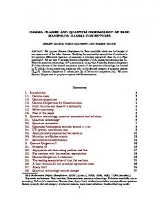
Example (4.5) Let T be the tangle on the left of Figure 1. It can be closed up to form a link L in S 1 × S 2 . B(T ) is given by taking the bracket polynomial of δh δ 2 A6 , the matrix of link diagrams on the right of Figure 1. Thus B(T ) = 2 δ h w where h = −δ(A4 + A−4 ), the bracket of the standard diagram for the Hopf link, and w = −2 + A−16 − A−8 − A−4 − 2A4 − 2A8 − A20 . Kauffman has a good method for calculating the bracket of link diagrams with double strands [KL,(§4.4)]. See also [K2], an early version of [K3]. We call this the Kauffman double bracket method. We used this method to calculate w. Thus Q(T ) is given by −1 − A−4 −A−2 + A6 A−10 − A−6 + 3A−2 + A2 − A6 + 2A10 − A14 A−12 − A−8 + 2 − 2A4 + A12 − A16 This matrix has a nonzero determinant D(L) = −A−16 + A−12 + 2 − 2A4 − A16 + A20 . Thus the above matrix represents z(L), and Γ(L) = g0 + g1 x + x2 where g0 = D(L) above and g1 = −A−12 + A−8 + A−4 − 1 + 2A4 − A12 + A16 . We may conclude that the wrapping number of L is four. This also follows from [Li], as well as [HP]. Using (1.5) and an analog of (3.4), we conclude that L is not isotopic to its image under a orientation reversing diffeomorphism of S 1 × S 2 ignoring banding. If X is either a scalar in Z[A] or a matrix over Z[A], then we let either p X or Xp (depending on where there is more room for the subscript) denote X after evaluating at A = Ap . Similarly if X is a module or module homomorphism over Z[A, A− 1] or Q[A, A−1 ] let Xp denote the result of tensor product with kp or Idkp . We will say p is ordinary with respect to n if and only if D(n)p is nonsingular. If p is not ordinary, we will say it is special with respect to n. Ko and Smolinsky


15

[KS] studied the question: when is p ordinary with respect to n? We note first that since det D(n) is a nonconstant polynomial almost all p are ordinary with respect to a given n. Ko and Smolinsky showed that all the roots of D(n)p are of the form δ = kπ ) where 1 ≤ k ≤ m ≤ n. We note that one and two are ordinary with 2 cos( m+1 respect to any n. Ko and Smolinsky showed that 2r is special with respect to r − 1, as required by Lickorish [L2]. By [BHMV1,(1.9)], there is an epimorphism ǫ(D3 ,2n) : K(D3 , 2n)p → Vp (S 2 , 2n). Here we let (S 2 , m) denote the 2-sphere with m framed points. Using the nonsingular Hermitian form on Vp (S 2 , 2n), one sees that ǫ(D3 ,2n) is an isomorphism if and only if p is ordinary with respect to n. In this case {Di } describes a basis for Vp (S 2 , 2n) with cardinality c(n). [BHMV1,(4.11 & 4.14)] gives bases for Vp (S 2 , 2n) and so may also be used to determine when ǫ(D3 ,2n) is an isomorphism. We obtain: Proposition (4.6). If p ≥ 4 is even, then p is ordinary with respect to n if and only if p > 2n + 2. If p ≥ 3 is odd, then p is ordinary with respect to n if and only if p > n + 1. Theorem (4.7). If p is ordinary with respect to n, and D(L)p 6= 0, then Γp (L) = (Γ(L))p , and zˆp (L) = z(L)p Proof. If p is ordinary with respect to n, Zˆp (I × S 2 , T ) with respect to the basis {Di } is represented by the matrix Q(T )p . If D(L)p 6= 0, then (Q(T )♮ )p represents Zˆp (I × S 2 , T )♭ . We note that the hypothesis of (4.7) is true for almost all p if Γ(L) 6= 0. Although it would be interesting to calculate zp (L), or zˆp (L) for p which are special with respect to n, we do not pursue this now. In order to define invariants for odd links in S 1 × S 2 we have several options. One could color the link L with a fixed even integer, say two, and evaluate the above invariants in the colored theories. Alternatively one could consider the link obtained by replacing each component of L with two strands using the banding to form a new banded link L′ , and then calculate the invariants of the even link L′ . Note that L′ is formed by taking a pair of “scissors” and splitting each band in L to form two bands. One could use other “even” satellite constructions. In §10 we will mention a third method of obtaining invariants of odd links. §5 Knot invariants Given an oriented knot K in a homology sphere S, we may let S(K) denote zero framed surgery to S along K. S(K) has the integral homology of S 1 × S 2 . We let χ denote the cohomology class which evaluates to be one on a positive meridian of K. Let Zp (K) denote Zp (S(K), χ), Zˆp (K) denote Zˆp (S(K), χ), and Γp (K) = Γp (S(K), χ). We will also let E(K) denote the list of eigenvalues of Zˆp (K) counted with multiplicity. By Proposition (1.5), one can see that these invariants do not depend on the string orientation of the knot. Let −K denote the knot obtained by taking the mirror image of K and reversing the string orientation. This knot represents the inverse of K in the knot cobordism group. Then Zp (−K) = (Zp (K))∗ . Let U denote the unknot in S 3 , then S 3 (U ) = S 1 × S 2 . So far for the examples we have calculated Zˆp (K) is diagonalizable. It would be interesting to

16

PATRICK M. GILMER

find two knots K1 and K2 such that Γp (K1 ) = Γp (K2 ), but Zˆp (K1 ) 6= Zˆp (K2 ), or Zp (K1 ) 6= Zp (K2 ). Theorem (5.1). If K is a fibered knot in a homology sphere which is a homotopy ribbon knot, then one is a root of Γp (K). Proof. According to Casson and Gordon [CG1], a fibered knot in a homology sphere is homotopy ribbon if and only if the the closed monodromy extends over a handlebody H. In this case the ordinary mapping torus R of the extension to the handlebody is a homology S 1 × B 3 which embeds naturally in a homology ball B with boundary S in which K bounds a homotopy ribbon disk ∆. In fact R is basically the exterior of ∆. We can give B a p1 -structure.. It will induce a p1 structure on R which in turn induces a p1 -structure on S(K) with σ zero. Note H represents an element in V (∂H) = V (Σ) which is fixed by T . Thus H represents an eigenvector with eigenvalue one. Remark Although there is an algorithm to answer the question of whether a given diffeomorphism extends over a handlebody [CL], consideration of the eigenvalues of a map induced under a TQFT functor may turn out to be a good way to show that a diffeomorphism does not extend over a handlebody or even bound in the bordism group of diffeomorphisms [B],[EW]. The following proposition follows instantly from [BHMV1,(1.5)]. Here ip : k2 → k2p and jp : kp → k2p are the homomorphisms defined in [BHMV1]. We must note that for p odd, ip (κ2 )jp (κp ) = κ2p . We use the same symbols to describe the induced maps on similarity classes and polynomials over these rings. We will discuss the tensor product of polynomials in the Appendix. Proposition (5.2). If p is odd, then Z2p (K) = ip (Z2 (K)) ⊗ jp (Zp (K)), and so Γ2p (K) = ip (Γ2 (K)) ⊗ jp (Γp (K)). Let U denote the unknot. We will say the similarity class of the identity on a free module of rank one is trivial. Theorem (5.3). For all p, Zp (U ) is trivial. If p is one, three or four, and K is a knot in S 3 , then Zp (U ) is also trivial. Proof. The first statement follows directly from the definitions. If p is one, three or four, we have [BHMV1,§2][BHMV2,§6] ω = η, κ−3 η = 1, κ6 = 1, and thus κ3 η = 1. One may obtain any knot in S 3 from the unknot U by doing ±1 surgery to the components of an unlink in the complement of U where the linking number of each component with U is trivial [R,(6D)]. Thus we may pick a Seifert surface F for U in the complement of this unlink. We may calculate Zp (U ) from an E that we construct with Σ = F capped off. Here we give S 3 a p1 -structure with σ zero. Let us calculate the effect of a single surgery on E. Let E ′ denote the result of performing +1 framed p1 -surgery to E. Then Zp (E ′ ) = ωp Zp (E) = ηZp (E). Let K ′ denote the image of U after this surgery. Then Zp (K ′ ) = κ−3 Zp (E ′ ) = Zp (E) = Zp (U ). If we were to perform −1 surgery then the invariant would change by a factor of κ3 η = 1. This same argument may be repeated to show the further surgeries do not change Zp (K). In order to obtain (5.6) below about periodicity of Zp (K), for K fibered with periodic monodromy, we make the following definitions and observations which will be useful later as well. Let σω (K) = Sign((1 − ω)V + (1 − ω ¯ )V t ), where ω ∈ C


17

with |ω| = 1 and V is a Seifert matrix for K. Following [KM2], let σd (K) = Pd−1 2πi/d . These are called the total d-signatures of K. i=1 σωdi (K), where ωd = e Our convention is that σ1 (K) is taken to be zero. Also def(S 3 (K), χd ) = −σd (K). By (3.5) we have: Proposition (5.4). Let α(K, d) be the p1 -structure on S(K)d induced from S(K), σ(α(K, d)) = 3σd (K). Lemma(5.5). If K is a fibered knot with a periodic monodromy of order s, then σs+1 (K) ≡ 0 (mod 8), and σs (K) ≡ 0 (mod 8). Proof. Let Dd denote the d-fold cyclic branched cover of D4 along a pushed in Seifert surface for K. Dd is a spin simply connected manifold with boundary Kd and Sign(Dd ) = σd (K). Ks+1 is the result of 1/n surgery on K for some n. Thus Ks+1 is a homology sphere. So the signature of Ds+1 is the signature of an even unimodular symmetric matrix and so is zero modulo eight. (S 3 (K))s is diffeomorphic to Σ × S 1 . It follows that H1 (Ks ) is torsion free. Thus the induced form on H2 (Ds ) modulo the radical of the intersection form is given by an even unimodular symmetric matrix and so has signature zero modulo eight. Proposition (5.6). Suppose K is a fibered knot with a periodic monodromy of order s. Let u4(σs (K)/8) have order h in kp . Note h divides p. Then Zp (K) is a periodic map with period hs. Proof. By(5.4), κσ(α(K,d)) = u4(σs (K)/8) . The result follows from the proof of (3.10). 2k+1 J k full twists

2k+1

k full twists Figure 2

2k+1

J

Given a surgery description of a knot as in Rolfsen [R,159] where each surgery curve has zero linking number with the unknot, we will give a procedure to calculate Zp (K). We use Rolfsen’s method of giving a surgery description for the infinite cyclic branched cover of S 3 along K from a surgery description for K [R, p162, p158]. The same picture and argument shows that we are obtaining a description of the infinite cyclic unbranched cover of M (K) as obtained by surgery to R × S 2 . Since we are actually working with manifolds with a p1 -structure our surgery is p1 surgery, but when we do our initial surgery to tie up K we change the p1 -structure on S 3 and S 1 ×S 2 . In other words our surgery description describes M (K) with the p1 -structure with σ3 equal to the number of plus one surgeries minus the number of ′ minus one surgeries done [BHMV1, Appendix II]. We have Zp (K) = κ−σ p ZP (E (Σ)), where E ′ (Σ) is the manifold we describe below.

18

PATRICK M. GILMER

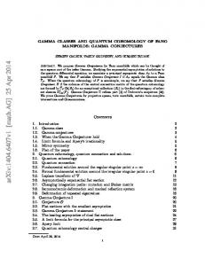
Twisted Doubles of Knots. We consider first the case that K is Dk (J), the k-twisted double of a knot J [R,p112]. We perform a single minus one surgery to undo the clasp. See [CG2], [K1,Chapt 18] where the (finite) cyclic covers are calculated for J the unknot, and [R] for k = 0 and J equal to the right handed trefoil. Figure 2 gives a surgery description for the infinite cyclic cover (with k = 4). The box labelled J represents two parallel copies of a string diagram for J with zero writhe. To obtain the infinite cyclic cover one should perform framed surgery to R×S 2 along the indicated infinite chain. Consider a 2- sphere given by {a} × S 2 which meets one component of our diagram in two points. Delete these two points and close the surface off by adding a tubular neighborhood of an arc on the intersected component. Call the resulting torus Σ.

ω

2k+1 f ull twists

k full twists

Figure 3

We can now construct E ′ (Σ) by taking a “slab” I × S 2 , drilling out a tunnel along an arc which meets {0} × S 2 (the arc is the top of one of the surgery curves), adding a 1-handle added along {1} × S 2 , and finally performing framed surgery along a simple closed curve γ which travels once over the one handle. According to [BHMV1,(1.C),§2,(5.8)], Zp (E ′ (Σ)) = Zp (E ′′ (Σ)), where E ′′ (Σ) is formed by placing a linear combination of banded links ω with 2k + 1 full twists along γ where we would have performed surgery in constructing E ′ (Σ). In Figure 3, we sketch E ′′ (Σ) when J is the unknot. The figure actually shows the case k = 2. We only draw an I × B 2 portion of I × S 2 . Given an element in α ∈ V (Σ), we may figure out its image under Zp (E ′′ (Σ)) as follows. α can be represented by a banded link in a solid genus one handlebody H with boundary Σ. If we glue this handlebody to the bottom of E ′′ (Σ) we will obtain a linear combination of banded links in the handlebody H ∪ E ′′ (Σ) with boundary T (Σ). This linear combination is formed as the union of α and ω. This linear combination represents Zp (E ′′ (Σ))(α) ∈ V (T (Σ)). Preparatory material on the Kauffman bracket and the Kauffman polynomial. Let ck (J) denote the bracket of the diagram, say Dk (J), obtained from a diagram of a knot J with writhe k by replacing each arc by 2 parallel arcs. The Kauffman double bracket method is a very efficient means for calculating ck (J). In fact ck (J) =


19

[Dk (J)]2 + 1, [KL,(p.35-36)] and [ ]2 satisfies a simple skein relation. We let [[J]] denote [D0 (J)]2 . Note [[J1 #J2 ]] = δ21−1 [[J1 ]] [[J2 ]]. Also ck (J) = A8k [[J]] + 1. If D is a knot diagram, then the writhe of D, denoted w(D) is well defined. This is not true of link diagrams. One may show that < D >2 = iw(D) 2. If J is a knot, let < J > denote the bracket polynomial of a diagram for J with zero writhe. Thus < J >2 = 2. Using the relation of the bracket polynomial and the Jones polynomial, it is easy to see that < J > will be a polynomial in even powers of A. It is convenient to note that [K5,(3.2)] < J >=

a + a−1 − 1 FJ (a, z)|a=−A3 z

and z=A+A−1

Here FJ (a, z) denotes the Kauffman polynomial, normalized so that it is one for the unknot. This is the form that is in the tables of [K1]. As observed in [KL], [D]2 is the Dubrovnik version of the Kauffman polynomial [K5,§VII] of D evaluated at z = A4 − A−4 , and a = A8 . Using Lickorish [L4], we have: [[J]] = −

a + a−1 − 1 FJ (a, z)|a=−iA8 z

and z=i(A4 −A−4 )

Let bk (J) denote the bracket of D0 (J) but with k additional full twists between the two strands. One has that bk (J) = A−6k ck (J) = A2k [[J]] + A−6k . The following proposition now follows easily from the above formulas. This proposition seems related to identities in [P] and could perhaps be proved using them. Proposition (5.7).

p bk (J)

is periodic in k with period p. Also 2 bk (J) = (−1)k 4.

Some conventions which hold for the rest of this paper. We will let A denote Ap , unless there may be some confusion as to which p is meant. We do not specify which primitive 2pth root of unity this is. Similarly Ω, ω, κ, δ will denote the items defined in [BHMV1], and sometimes denoted Ωp , ωp , κp , δp . We let µ = µ(1) = −A3 . We also give κ−3 η the name β. We also let bk (J) denote bk (J) evaluated at Ap , and < J > denote < J >p The case p = 2. If Σ is a torus, then V2 (Σ) has a basis consisting of 1 and z. We have that ω = ηΩ where Ω = 1 + z2 , and β = 1−A . With respect to the basis {1, z}, 2 1 Z2 (E(Σ)) = κ−3 Z2 (E ′′ (Σ)) is given by β µ2k+1 µ2k+1 bk (J) . Thus Z2 (E(Σ)) 2δ 2δ 1 2 1−A is given by 2 . A (−1)k A 2 Proposition (5.8). Let K be the k twisted double of J. If k is even, then Z2 (K) 1 2 , and Γ2 (K) is x2 −x+1. So E2 (K) is trivial. If k is odd, Z2 (K) = 1−A 2 − A2 A ♮ is {1} if k is even and is {A3 , A¯3 } if k is odd.

20

PATRICK M. GILMER

The case p = 5. If Σ is a torus, then V2 (Σ) has a basis consisting of 1 and z. We have ω = ηΩ. 2 −2A3 Ω = 1 + δz, and β = 3−A+4A . With respect to the basis {1, z}, Z5 (E(Σ)) = 5 1 κ−3 Z5 (E ′′ (Σ)) is given by β . 2k+1 2k+1 µ µ bk (J) By Proposition (5.7), each entry in the above matrix has period five. Thus: 1 Proposition (5.9). Z5 (Dk (J)) = β . Z (D (J)) µ2k+1 < J > µ2k+1 bk (J) ♮ 5 k is periodic in k with period five. We now calculate these five invariants for various knots J. First we consider J = U , the unknot. We can make a number of predictions a priori. Note that D0 (U ) is the unknot again, so Z5 (D5n (U )) is trivial. Also note D1 (U ) is the figure eight knot and D−1 (U ) is right handed trefoil. Both of these knots are fibered, so E5 (D5n+1 (U )) and E5 (D5n−1 (U )) should consist of elements of norm one. Since the trefoil is period with period six, by (5.4), E5 (D5n+1 (U )) should consist of 30th roots of unity. Also since the figure eight is amphichiral, E5 (D5n+1 (U )) = E5 (D5n+1 (U )). We obtain: Proposition(5.10). If k ≡ 0 (mod 5), Z5 (Dk (U )) is trivial. If k 6≡ 0 (mod 5), 1 δ Z5 (Dk (U )) = β . In particular for all in2k+1 2k+1 2k 2 µ δ µ (A (δ − 1) + A−6k ) ♮ tegers n, we have: Γ5 (D5n (U)) = x − 1

E5 (D5n (U)) = {1}

¯ +1 Γ5 (D5n+1 (U)) = x2 − (A + A)x 2 ¯ +A ¯ Γ5 (D5n+2 (U)) = x − (1 + A)x

¯ E5 (D5n+1 (U)) = {A, A} ¯ E5 (D5n+2 (U)) = {1, A}

¯2 )x + A ¯ Γ5 (D5n+3 (U)) = x2 − (1 + A 2 2 ¯ ¯ Γ5 (D5n+4 (U)) = x − (A)x + (A)

¯ A ¯3 A}. ¯ E5 (D5n+4 (U)) = {A3 A,

Note E5 (D5n+4 (U )) are primitive 15th roots of unity. We do not list the eigenvalues for the 5n + 3 twisted doubles. Although they are easily worked out, the formulas are not enlightening. By (5.1) and (5.10), we have that the trefoil and figure eight knots are not homotopy ribbon. This a (not very deep) four dimensional result obtained from studying a TQFT in dimension 2+1. By (7.6), below we have that the granny knot is not homotopy ribbon as well. Let RT, LT and F 8 denote the right handed trefoil, the left handed trefoil and the figure eight knots. For J = RT , LT F 8, and the square knot RT #LT and for all k, the above matrix has nonzero determinant. Below we list {k, Γ5 (D5n+k (J))} for J = RT, LT, F 8, and RT #LT. J = RT {0, 1 + 2 A2 − 2 A3 − 2 − A + 2 A2 − A3 x + x2 } {1, −A3 − 2 − A3 x + x2 } {2, 1 + A − A2 − 1 − A + A2 − 2 A3 x + x2 } {3, 1 − 2 A − A3 − (1 − A) x + x2 } {4, −A + A2 + A3 − A x + x2 } J = LT


21

{0, 2 − 2 A − A3 + A3 x + x2 } {1, −1 − A + A2 − 1 − A + A2 x + x2 } {2, 1 + 2 A2 − A3 − (1 + A) x + x2 }

{3, A − A2 − A3 − 2 − A + 2 A2 − 2 A3 x + x2 } {4, 1 − 2 − A − A3 x + x2 } J = F8

{0, −3 + 2 A − 2 A2 + 3 A3 − A2 x + x2 } {1, 3 + 2 A2 − A3 − 2 + A2 x + x2 } {2, 1 − 2 A − A3 − 2 + A2 − 2 A3 x + x2 } {3, 1 + 2 A2 − A3 − 2 − 2 A + A2 − 2 A3 x + x2 } {4, 1 − 2 A − 3 A3 + A2 x + x2 }

J = RT #LT {0, −6 + 4A − 4A2 + 6A3 − A − A2 + 2A3 x + x2 } {1, 6 + A + A2 − 1 + A + 2A2 − A3 x + x2 } {2, 1 − 5A + A2 − 2A3 − 4 − 2A + 2A2 − 2A3 x + x2 } {3, 2 − A + 5A2 − A3 − 1 − A2 − 2A3 x + x2 } {4, −A − A2 − 6A3 − −2A + A2 − A3 x + x2 }

The case p = 6. By (5.2), Z6 (K) = i3 (Z2 (K)) ⊗ j3 (Z3 (K)). Note that i3 (A2 ) = A96 = −A36 . As Z3 (K) is trivial, and ip fixes Z, we have by (5.8) that: Proposition(5.11). Z6 (K) = i3 (Z2 (K))). if k is even Z6 (Dk (J)) In particular, 3 1 2 , and Γ6 (K) = x2 − x + 1. is trivial. If k is odd, Z6 (Dk (J)) = 1+A A3 3 2 −A 2 ♮ So E6 (Dk (J)) is {1} if k is even and is {A3 , A¯3 } if k is odd. The case p = 10. By (5.2), we have Z10 (K) = i5 (Z2 (K))⊗j5 (Z5 (K)), and so Γ10 (K) = i5 (Γ2 (K))⊗ j5 (Γ5 (K)). Thus one may work out, for instance, Γ10 (Dk (U ). We note that j5 (A5 ) = A610 . By (5.8) and (5.10), i5 (Γ2 (D5n+4 (U ))) = x2 − x + 1, and j5 (Γ5 (D5n+4 (U ))) = x2 + (A410 )x + A810 . Using A.3 from the appendix, we obtain:

(5.12)

Γ10 (D5n+4 (U )) = x4 + (A410 )x3 − (A210 )x − A610 .

The general case, p ≥ 3. Pn−1 If p ≥ 3 then ω = ηΩ, and Ω = s=0 < es > es where es is an eigenvector for the 2s+2 −2s−2 2 twist map with eigenvalue µ(s) = (−1)s As +2s , and < es >= (−1)s A A2 −A . −2 −A p−1 n−1 The {ei }i=0 where n = 2 form a basis for V of a torus. We form two n × n Pn−1 matrices B(J, k) and L(J). B(J, k)i,j = β s=0 < es > µ(s)2k+1 b(J, k)i,s,j where

22

PATRICK M. GILMER

b(J, k)i,s,j is the bracket polynomial of the colored banded link in Figure 4a.

i

s

J

i

J(k)

j j

J

Figure 4a

Figure 4b

The box labelled J(k) represents two parallel strands of a string diagram for J with zero writhe with k additional full twists added to the strands and the circle labelled J represents a string diagram for J with zero writhe. Let L(J)i,j be the bracket polynomial of the colored banded link in Figure 4b. For a knot J, let Jc denote J colored c. Theorem (5.13). If p ≥ 3, and < Jc >p is nonzero for all 0 ≤ c ≤ n − 1, then Zp (Dk (J)) = (B(J, k) L(J)−1 )♮ . b(J, k)i,s,j and L(J)i,j may be calculated recursively using the colored Kauffman relations. These are given in [MV2] and for p even in [KL]. In fact L(U )i,j for p even is given in [KL,p.127]. This is easily worked out for all p using the formulas in [MV2]. It is not hard to see that the summations given [MV,p 367] should be taken over k such that (i, j, k) is a small admissible triple, when one specializes to A = Ap . Using the colored Kauffman relations, one may deduce: Corollary (5.14). If p ≥ 3, and < Jc >p is nonzero for all 0 ≤ c ≤ n − 1, then Zp (Dk (J)) is periodic in k with period p. Let δ(k; i, j), and < i, j, k > be as in [MV2]. We have: (5.15)

L(U)i,j =

X

δ(r; i, j)2 < r > .

r ∋ (i,r,j) is a small admissible triple

(5.16) b(U, k)i,s,j =

X

r,r′ ∋ (i, r, s), and (j, r′ , s) are small admissible triples

δ(r; i, s)2 δ(r′ ; j, s)2k

< r >< r′ >

Of course both of these should be evaluated at A = Ap . We have calculated Zp (Dk (U )) exactly with entries polynomials in A for 0 ≤ k ≤ p − 1 and for 5 ≤ p ≤ 16. These as well as other lists of quantum invariants are available at gopher://math.lsu.edu. For certain knots, we have carried the calculation to higher p. We observe that for p ≤ 20, Zp (RT ) is a periodic map with period 3p, and sometimes less. By (5.6), Zp (RT ) must be periodic with period by 6p, and sometimes less, since the trefoil has a monodromy of period six. The roots of Zp (F 8) are all periodic maps for p ≤ 20. The period is an erratic function of p. This periodicity is somewhat surprising since the monodromy for F8 is hyperbolic. We also


23

observe that Γp (61 ) has one as an eigenvalue one for p ≤ 18. The tweenie knot is 52 = −D2 (U ) [As,p.86]. We noticed that the degree of Γ2r ( tweenie knot ) is less than r − 1 = dim V2r ( torus ) for 3 ≤ r ≤ 9. Thus the hypothesis of (2.7) does not hold. We plan to investigate whether I(M, χ) is principle in this case. Other Knots K. If we consider more general knots, two extra difficulties arise. First, we may not be able to calculate Zp (E(Σ)) directly but only some power of it. As an example, starting with the surgery description of the knot 816 given in [R,p.169], one may calculate Zp (E(Σ))n for n ≥ 2. Fortunately if we can calculate Zp (E(Σ))c, then we can also calculate Zp (E(Σ))c+1 , and from this deduce Zp (E(Σ))♮. Secondly, the genus of Σ may be higher than one. In the higher genus case, there is a good description [MV1],[BHMV1] of a basis of Vp (Σ) in terms of colorings of a trivalent graph which is a deformation retract of the handlebody. Thus the same methods may be applied. The calculation becomes more difficult as p and the genus of Σ grow. A computation with Σ genus two. V5 of the boundary of a genus two handlebody has a basis given by the links denoted 1, z, w, zw, and z#w in Figure 5. Starting with a surgery description of the knot 88 , we obtain, as in Rolfsen, a surgery description of the infinite cyclic cover shown in Figure 6. Just as above, we can then find a matrix for calculating Z5 (88 ). In particular, we have that Γ5 (88 ) = (x − 1)(x4 + (−1 − A − A2 )x3 + (1 + A2 )x2 + (−A − A2 − A3 )x + (−1 + A + A3 )).

1

z

w

z #w

zw

Figure 5 -3 +1

-3 +1 Figure 6

§6 Quantum Invariants of the finite cyclic covers of S 3 (K) For p ≥ 3, (1.8), and the remarks following tell us how to compute < S 3 (K)d >p recursively as a function of d, once we know Γp (K). We discuss < S 3 (K)d >p for low p. We have that < S 3 (K)d >p = 1, for p = 1, 3, and 4. For p = 1, this follows easily from the definitions. For p = 3, and 4, this follows from (1.8) and (5.3). By (1.7) and (5.9) (6.1)

< S 3 (Dk (J)) >5 = β5 (1 + µ52k+1 bk (J)5 ).

24

PATRICK M. GILMER

By (1.8) and (5.11)  1      2 3 < S (Dk (J))d >6 = 1    −1    −2

(6.2)

if k is even if k is odd and d ≡ 0 (mod 6) if k is odd and d ≡ ±1 (mod 6) . if k is odd and d ≡ ±2 (mod 6) if k is odd and d ≡ 3 (mod 6)

We let s(k, d) denote the function above. Again as Z2 does not satisfy the tensor product axiom, we need an alternative method of calculating < S 3 (K)d >2 . < S 3 (K)d >2 can be computed from < S 3 (K)d >6 using [BHMV1,1.5] since < S 3 (K)d >3 = 1. In fact, one sees that < S 3 (K)d >2 is equal to the sum of the dth powers of the roots of Γ2 (K). Thus it turns out that < S 3 (K)d >p is the sum of the dth powers of the roots of Γp (K), for all p ≥ 1. In particular, < S 3 (Dk (J))d >2 = s(k, d).

(6.3) Thus we have

< S 3 (Dk (J))d >10 = s(k, d)j5 (β5 (1 + µ52k+1 bk (J)5 )).

(6.4)

Here are some examples for p = 5. All of these examples are atypical except perhaps the last. In the first of these examples, we compare our result with previous calculations. The covers of 0-surgery along the trefoil. By (5.10) the eigenvalues of Z5 (RT ) are primitive 15th roots of unity. Thus < S 3 (RT ))d >5 is periodic with period fifteen. Actually the first fifteen values are −A4 , A3 , 2 A2 , A, −1, −2A−1 , A3 , −A2 , −2 A, −1, A−1 , −2 A3 , −A2 , A, 2. Since the monodromy of the trefoil has order six, one might, at first, expect periodicity of order six. However by (5.4), < S 3 (RT ) >5 = κ−3σ7 (RT ) < (S 3 (RT ))7 >5 = −A4 . This is consistent with our previous calculation of < S 3 (LT ) >5 . S 3 (RT )6 is the three torus. Thus the invariant of the three torus equipped with a p1 -structure α with σ(α) zero is κ−3σ6 (RT ) < (S 3 (RT ))6 >5 = κ24 (−2A−1 ) = 2. This calculation agrees with (3.9). The covers of 0-surgery along the untwisted double of the figure eight knot. < S 3 (K)d >5 is given by the sum of the dth powers of the roots of Γ5 (K) counted with multiplicity. It may also be easily computed recursively. This example is atypical in that we noticed something systematic. Γ5 D0 (F 8) = x2 − (A2 )x + (−3 + ¯ − 8(A2 + A¯2 ) − 1. λ is a positive real number 2A − 2A2 + 3A3 ). Let λ = 12(A + A) πi under all complex embeddings of κ5 . In fact if A goes to e± 5 , then λ goes to 3πi approximately 13.4721. If A goes to e± 5 , then λ goes to approximately 4.52786. Let κ be the positive square root of λ. Then the roots of Γ5 (D0 (F 8)) are 1+κi 2 , 1−κi and 2 . So we have: (6.5) 3

< (S (D0 (F 8)))d >5 =

A2d 2d

[d/2] A2d X r d ((1 + κi) + (1 − κi) ) = d−1 λr (−1) 2 2r r=0 d

d


25

The behavior of the argument (or phase) of < (S 3 (D0 (F 8)))d >5 mod π as a function of d is quite simple in this case. The covers of 0-surgery along the knot 81 . This example is more typical. The 3-twisted double of the unknot is 81 . One may of course easily compute < (S 3 (81 ))d >5 exactly by recursion. For example < (S 3 (81 ))17 >5 = 188 + 152A + 136A2 . There is not much pattern. However πi if we embedd k5 in C by sending A to e 5 then the eigenvalues of Z5 (81 ) are e1 ≈ 0.676766 − 1.2548i, and e2 ≈ .632251 + 0.303739i. e1 has norm greater than one and e2 has norm less than one. Thus < (S 3 (81 ))d >5 = (e1 )d + (e2 )d . So d πi ≈ (e1 ) , for d large. < (S 3 (81 ))d >5 5 |A=e

§7 A connected sum formula If c is a q-color, let K(c) denote S(K) with the image of a meridian colored c. Here and below the banding on a meridian is taken to be that given by another nearby meridian. As before we have a generator χ ∈ H 1 (S(K)). Let Zp (K, i) = Zp ((K, i), χ). Define Γp similarly. Note Zp (K, 0) = Zp (K). Since Vp of a surface with a single odd colored banded point is zero, Proposition (7.1). If c is odd, Zp (K, c) = 0 Because Vp of a 2-sphere with a single colored banded point is zero, we have: Proposition (7.2). If c 6= 0, Zp (U, c) = 0 Let U (i, j, k) denote zero surgery to the unknot with the images of three meridians colored i, j, and k, where these are are good q-colors. By [BHMV1,(4.4)], Vp of a 2-sphere with three points colored i, j, and k, is one dimensional if (i, j, k) is a small admissible triple, and is zero otherwise. Thus Proposition (7.3). Assume p ≥ 3. Zp (U, i, j, k) is the identity on a free rank one kp -module if (i, j, k) is a small admissible triple, and is zero otherwise. By (7.3), and the Colored Splitting Theorem [BHMV1,(1.14)], one has: Theorem 7.4. Assume p ≥ 3. Zp (K1 #K2 ) =

M

Zp (K1 , i) ⊗ Zp (K2 , i).

i is a q-color

More generally: Zp (K1 #K2 , i) =

M

Zp (K1 , j) ⊗ Zp (K2 , k).

j,k such that (i,j,k) is a small admissible triple

Proposition(7.5). Z5 (Dk (U ), 2) is periodic in k with period five. In particular, Z5 (D5n (U ), 2) = [0]♮ Z5 (D5n+1 (U ), 2) = [1]♮ Z5 (D5n+2 (U ), 2) = [1 − A3 ]♮

26

PATRICK M. GILMER

Z5 (D5n+3 (U ), 2) = [1 − A − A3 ]♮ Z5 (D5n+4 (U ), 2) = [−A2 ]♮ Proof. One may use the same basic procedure described in §5 to calculate the colored invariants of a knot. One only needs to add a straight colored line to the slab. V5 of a torus with one framed point colored 2 is one dimensional [BHMV1,(4.14)]. A generator is pictured in Figure 7. To calculate Z5 (Dk (U ), 2) one should attach the solid handlebody of Figure 7 to the bottom of the slab of Figure 3 with a vertical line colored 2 added so that the arcs labelled 2 match up. This new picture represents some multiple of the generator pictured in Figure 7. Just as in §5 we must multiply by κ−3 to correct for the p1 -structure. Recall ω = η(1 + δz). But this diagram with the curve labelled ω deleted will represent zero since f2 times ⊃⊂ is zero in the Temperley Lieb algebra. Thus Z5 (E) is multiplication by ηδµ2k+1 times ak , where ak is the multiple of Figure 7 represented by our picture with curve label ω colored 1 and the 2k + 1 twists deleted. One may calculate ak doing a standard Kauffman bracket calculation of the link in the diagram colored 1, discarding any terms in an expansion where the segment labelled 2 is joined to a loop which is inessential (again since f2 times ⊃⊂ is zero.) One is left with ak times the generator. One has ak = A2 ak−1 + (1 + A)µ2−2k , and a0 = 0. The result follows easily.

1 2

Figure 7

The above result may also be derived from (7.7),(7.9) and (7.10). It also follows from (8.6) below. The above proof is more elementary and helps us understand these invariants concretely. By (5.10),(7.4) and (7.5), we have for instance:

E5 (RT #LT ) = {1, 1, 1, A23, A¯23 } E5 (F 8#F 8) = {1, 1, 1, A2, A¯2 } (7.6)

E5 (RT #RT ) = {A4 , A¯2 , A¯2 , A23 A¯2 , A¯23 A¯2 }

Before we made this calculation, we had found E5 (F 8#F 8) using the method used in calculating Γ5 (88 ). Let S(c, p) be the set of good q-colors i such that (i, i, c) form a small admissible triple. The colored graphs in the solid torus pictured in Figure 7 with 1 replaced by i and 2 replaced by c as i ranges over S(c, p) forms a basis for Vp of a torus with a single point colored c, [BHMV1,(4.11)]. Let n(c, p) be the cardinality of S(c, p). We form two n(c, p) × n(c, p) matrices B(J, k, c) and L(J, c) with rows and columns indexed by S(c, p). At this point, we begin to suppress the dependence on Pn−1 p again. B(J, k, c)i,j = β s=0 < es > µ(s)2k+1 b(J, k, c)i,s,j where b(J, k, c)i,s,j is


27

the bracket polynomial of the colored banded link in Figure 8a.

i c

c

s

J

i

J(k)

j j

Figure 8a

J

Figure 8b

Let L(J, c)i,j be the bracket polynomial of the colored banded link in Figure 8b. Let J(e) denote the knot J colored e. Theorem (7.7). If p ≥ 3, and < Je >p is nonzero for all e ∈ S(c, p), then Zp (Dk (J), c) = (B(J, k, c)L(J, c)−1)♮ . By the same arguments as used for (5.14), we have : Corollary (7.8). If p ≥ 3, and < Je >p is nonzero for all e ∈ S(c, p), then Zp (Dk (J), c) is periodic in k with period p. A B E Using the tetrahedron coefficient , in the notation of [MV2] , we D C F have: (7.9) X

L(U, c)i,j =

r ∋ (i,r,j) is a small admissible triple

δ(r; i, j)2 < r > < r, i, j >

c r

j i

j i

.

(7.10) If (c, s, s) is not a small admissible triple, b(U, k, c)i,s,j = 0, otherwise b(U, k, c)i,s,j =

r,r′

X

(j, r′ , s)

∋ (i, r, s), and are small admissible triples

δ(r; i, s)2 < r > δ(r′ ; j, s)2k < r′ > < r, i, s >< r′ , j, s >< c, s, s >

c r

i s

i s

c r′

j s

j s

.

§8 Quantum invariants of branched cyclic covers of knots Let sd (K, c)p denote the sum of the dth powers of the roots of Γp (K, c). Note that in §6, we calculated sd (K, 0)p in several cases. The same methods, originally discussed in the remarks following (1.8), may be applied to calculate sd (K, c)p, from Γ(K, c). Proposition (8.1). If p ≥ 3 and c is even, sd (K, c)p =< K(c)d >p . Let Kd denote the branched cyclic cover of a knot K equipped with a p1 -structure α with σ(α) = 3σd (K). This is in the homotopy class of p1 -structures which extend across the branched cover of D4 along a pushed in Seifert surface. Recall < ei >= 2i+2 −2i−2 . (−1)i A A2 −A −A−2

28

PATRICK M. GILMER

Theorem (8.2). For p ≥ 3,

< Kd >p =

(

η η

P(p−3)/2 i=0

P[p/4]−1 i=0

< e2i > sd (K, 2i)p

if p is odd

< e2i > sd (K, 2i)p

if p is even.

Proof. Note that 0-framed surgery to S 3 (K)d along the inverse image of the meridian is actually Kd . The trace of this surgery has zero signature, so the σ invariant of the p1 -structure is the same for Kd and S 3 (K)d . Suppose we have a surgery description of K in S 3 . Consider the resulting surgery description of S 3 (K)d . Let Dc be the result of replacing each surgery curve by ω with the given framing and then adding to the resulting picture the inverse image of the banded meridian colored c. Let Dω be the result of replacing each surgery curve by ω with the given framing and replacing the inverse image of the banded meridian by ω. We have that < K(c)d >p = η < Dc >, and < Kd >p = η < Dw > . Thus by (8.1) if p ≥ 3 and c is even, < Dc >= η −1 sd (K, c). Here < X > just the Kauffman bracket of the linear combination of framed links X, after letting A = Ap . Of course instead of replacing a curve by ω, we could replace it by any other combination of framed links in S 1 × B 2 which represents the same element of Vp (S 1 × S 1 ). If p is even, and c is odd, then by (3.1) < K(c)d >p = 0. If p is even, we are P(p−4)/2 done since ω = ηΩ, and Ω = < ei > ei . For p odd, we replace ω by i=0 P(p−3)/2 ′ ω = η i=0 < e2i > e2i . One uses [BHMV2,6.3(iii)], to see that ω and ω ′ represent the same element in Vp of the boundary of a solid torus. If K is a knot in S 3 , then K1 is S 3 . Thus we have the following restriction on the colored invariants of K. Corollary (8.3). For p ≥ 3,

1=

( P(p−3)/2 i=0

P[p/4]−1 i=0

< e2i > Trace Zp (K, 2i)

if p is odd

< e2i > Trace Zp (K, 2i)

if p is even.

Since η3 = −1, we have the following corollary which may also be derived from (5.3). Corollary (8.4). < Kd >3 = −1 Corollary (8.5). < Kd >6 = η6 < S 3 (K)d >6 , and < Kd >2 = η2 < S 3 (K)d >2 . −1 In particular, < (Dk (J))d >2 = η2 s(d, k). Thus η10 < (Dk (J))d >10 = s(d, k)j5 (η5−1 < (Dk (J))d >5 ). Proof. The first equation is just (8.2) for p = 6. Applying [BHMV1, (1.5)] to S 3 with σ(α) = 0 we see ip (η2 )jp (ηp ) = η2p . The second equation follows from the first, i3 (η2 ) = −η6 , and (8.4). The third equation follows from the second and (6.3). The last equation follows from the third and [BHMV1, (1.5)] again. We may use (8.3) to obtain a generalization of (7.5). We note that when p is ¯ five, < e2 >−1 = −(A + A).


29

¯ Corollary (8.6). Z5 (Dk (J), 2) = [(A + A)(β(1 + µ2k+1 )bk (J) − 1)]♮ . In particular, Z5 (Dk (J), 2) is periodic in k with period five. For instance Z5 (D0 (F 8), 2) = [A3 + A4 ]♮ . In general, it is now an easy matter to calculate < Dk (J)d >5 recursively once we know < J >, and [[J]]. But these are just two values of the Kauffman polynomial, for which extensive tables exist. Moreover < Dk (J)d >5 is periodic in k with period five. We note that D2 (U ) is the stevedore’s knot 61 . We have for instance: ¯ d + (A¯3 A) ¯ d + (−1)d (1 − A + A4 )A2d η −1 < RTd >5 = (A3 A) η −1 < F 8d >5 = Ad + A¯d + (1 − A + A4 ) η −1 < (61 )d >5 = 1 + A¯d + (1 − A + A4 )(1 − A3 )d η −1 < (81 )17 >5 = 1175 + 762A + 1123A2 η

−1

[d/2] A2d X r d λr . (−1) < (D0 (F 8))d >5 = (1 − A + A )(A + A ) + d−1 2 2r r=0 4

3

4 d

¯ − 8(A2 + A¯2 ) − 1, as in (6.5). Note that < F 8d >5 is Here λ = 12(A + A) periodic in d with period ten. Also < RTd >5 is periodic in d with period thirty. This second periodicity is generalized below. Let θp denote the invariant of oriented closed 3-manifolds defined in [BHMV2]. Theorem (8.7). Suppose K is a fibered knot with a periodic monodromy of order s. Then < Kd >2 is periodic in d with period s. If p ≥ 3, then < Kd >p , and θp (Kd ) are periodic in d with period ps. If r ≥ 3, τr (Kd ) is periodic in r with period 2rs. If p = 2r with r odd and r ≥ 3, then < Kd >p and θp (Kd ) are periodic in d with period rs. If r is odd and r ≥ 3, then τr (Kd ) is periodic in r with period rs. Proof. The diffeomorphism type of S 3 (K)d is periodic in d with period s. It follows that the first Betti number b1 (< Kd >) = b1 (S 3 (K)d ) is periodic with period s. By [DK,(5.2)], σs+k (K) = σk (K) + σs+1 (K). By Lemma (5.5), σs+1 (K) ≡ 0 (mod 8), 3 so κ9σs+1 (K) = u 2 σs+1 (K) is also a pth root of unity. Thus κ3σ is periodic in d with period ps. In fact if p is even, κ3σ has period ps 2 . The first statement then follows from (8.5). Now suppose p ≥ 3. By (8.2), < Kd >p , will be periodic in d with period ps if the roots Γ(K, 2i)p are all psth-roots of unity. The underlying manifold of K(2i) is the mapping torus of the closed off monodromy on the fiber capped off, which we denote Σ. Σ has been given the structure of a banded point colored 2i, and K(2i) has been given the extra structure of a meridian colored 2i with a certain banding. Let E be the associated fundamental domain of the infinite cyclic cover of K(2i) and Es = ∪0≤i≤s−1 T i E as in §1. (Zp (E))s = Zp (Es ) is then given by a scalar multiple of the identity. This is because Es is diffeomorphic to Σ × [0, 1], forgetting extra structure. Note that K(2i)s has an induced p1 -structure with σ equal to 3σd (K). Whereas if we gave Σ × [0, 1] the product p1 -structure, then Zp (Σ × [0, 1]) would be the identity, and the associated mapping torus has a p1 -structure with σ equal to zero. See the proof of (6.10). Also the banding on the links in Es and K(2i)s differs by some number b of twists. Thus (Zp (E))s is κ9σs (K) µ(2i)b times the identity. Note µ(2i) is a pth-root of unity. By lemma (5.5), σs (K) ≡ 0 (mod 8).

30

PATRICK M. GILMER

So κ9σs (K) = (u2 )3σs (K)/4 is also a pth root of unity. It follows that (Zp (E))ps is the identity and all the roots of Γ(K, 2i)p are psth-roots of unity. By [BHMV1,§2], we have that θp (Kd ) are periodic in d with period ps. By [BHMV3,(2.2)], τr (Kd ) is periodic in r with period 2rs. If p = 2r where r is odd use [BHMV1,(1.5)] to express < Kd >p in terms of < Kd >r and < Kd >2 . This gives the above periodicity for < Kd >p . The periodicity of b1 (< Kd >p ), κ3 σ < Kd >, and [BHMV3,(2.2)] then yield the above periodicity of θp (Kd ) and τr (Kd ). Using Goldsmith’s construction [Go] of the fibration for T (a, b), the (a, b) torus knot, it is easy to see that the monodromy is periodic with period ab. K(a, b)c is the the Brieskorn manifold Σ(a, b, c) with a p1 -structure α such that σ(α) = 3σc (T (a, b). σc (T (a, b)) is equal to the signature of the variety z0a + z0b + z0c = 1 in C3 . There is a well known formula due to Brieskorn for this signature. Our convention is that Σ(a, b, c) is oriented as the boundary of the variety z0a + z0b + z0c = 1 intersected with the 6-ball. We have that < Σ(a, b, c) >p =< Σ(a, b, c + pab) >p (8.8)

τr (Σ(a, b, c)) = τr (Σ(a, b, c + 2rab)) if r is even < Σ(a, b, c) >2r =< Σ(a, b, c + rab) >2r if r is odd

(8.9)

τr (Σ(a, b, c)) = τr (Σ(a, b, c + rab)) if r is odd

Making use of the fact Σ(a, b, −c) = −Σ(a, b, c), one sees that these equations hold for all a, b, c positive or negative. In this way one obtains four further relations, for example: < Σ(a, b, c) >p = < Σ(a, b, pab − c) >p . The fact that the diffeomorphism type of Σ(a, b, c) is invariant under permutations of (a, b, c) leads to further relations among < Σ(a, b, c) >p . Freed and Gompf showed, for c of the form 6k ±1, that τr (Σ(2, 3, c)) was periodic in c with period 6r in the case r odd and with period 3r in the case r even. They used the fact that Σ(2, 3, 6k ± 1) is (∓1/k)-surgery on ±T (2, 3) and the periodicity of τr for (1/n)-surgery on a knot due to Kirby and Melvin. In (8.9) above, we generalize this periodicity for r odd. In (8.8), we get periodicity with four times this period. However we have no restriction on c in either case. Let vp (g, c) be the dimension of Vp of a surface of genus g with a single point colored c. We may use (3.8),(8.2), and the triangle inequality to obtain: Theorem(8.10). If K is a fibered knot with genus g, then for all d ( P(p−3)/2 i < e2i > vp (g, 2i) if p is odd i=0 −1 |i η (< Kd >p ) | ≤ P[p/4]−1 i < e2i > vp (g, 2i) if p is even. i=0 §9 Partial Invariance under skein equivalence The invariants which we discuss are almost invariant under skein equivalence. To see this, we first define some cobordism categories with more morphisms. We define Cˇ2p1 to be the cobordism category with objects those of C2p1 but whose morphisms are kp -linear combinations of morphisms of C2p1 between the same objects.


31

Composition is defined as follows. Suppose {Ci } is a finite set of morphisms from Σ1 to Σ2 and {Cj′ } is a finite set of morphisms from Σ2 to Σ3 , then {Ci ∪Σ2 Cj′ } is a finite set of morphisms from Σ1 to Σ3 . Define X

ai Ci ◦

i

X j

aj Cj′ =

X

ai bj (Ci ∪Σ2 Cj′ ).

i,j

We define Zp on Cˇ2p1 by extending linearly. One may define a expansion functor p1 ,c p1 ,c from C2,q to Cˇ2p1 , following the recipe in [BHMV1]. Similarly we define Cˇ2,q to be p1 ,c the cobordism category with objects those of C2,q but whose morphisms are kp p1 ,c linear combinations of morphism of C2,q between the same objects. We may define Zp (M, χ) if M is a morphism in these new categories from the ∅ to ∅ just as in §3. Let B be a basis for V (Σ), let M(M, Σ, B) denote the matrix for κ−σ(α(M )) Zp (E(Σ) with respect to B. Thus Zp (M, χ) = (M(M, Σ, B))♮ . Given a colored graph G in M transverse to a choice of Σ dual to χ, we may define the skein equivalence class of G modulo Σ to be the equivalence relation generated by ambient isotopies of G, which are the identity in a neighborhood of Σ and the local moves described in [MV2,§2] which takes place in the complement of this neighborhood. If G is really a link L (colored 1), one takes the usual Kauffman skein relation. We clearly have: Proposition (9.1). Let Σ be a fixed surface dual to χ, and B is a basis for Vp (Σ), M(M, Σ, B) is an invariant of the skein equivalence class of G modulo Σ. Thus, if Σ is some fixed surface dual to χ, Zp (M, χ) is well defined on the skein class of G modulo Σ. In a similar way, we have in the notation of §4: Proposition (9.2). Q(T ) is an invariant of the skein equivalence class of T . §10 Vp ((S 2 , m)

` 2 (S , 1)) and odd Links in S 1 × S 2

Here we discuss another approach to odd links. We let (S 2 , m) demote a 2-sphere 2 2 with m banded points (colored one). K(S ` ,2m) is zero for m odd, so V (S , m) 2 vanishes as well. Whenever V` (S ,m2 )) is nonzero, one may consider p ((S , m1 ) 1 2 1 2 zp (L, m2 ) = Zp (S × S , L) (S × S , Lm2 ) , where Lm denotes m S 1 - factors. As a first case, we consider zp (L, 1). It turns out that the few invariants we get in ` this case are very trivial. However our calculation of Vp ((S 2 , m1 ) (S 2 , 1)) may be of interest. ` ` Lemma (10.1). For p 6= 3 or 1, Vp ((S 2 , m) (S 2 , 1)) = ` 0. V3 ((S 2 , m) (S 2 , 1)) = kp if m is odd and is zero if m is even. dim(V1 ((S 2 , m) (S 2 , 1))) = c( m+1 2 ) if m is odd and is zero if m is even.

Proof. For p even and p greater than two, this follows since Vp ((S 2 , 1)) = 0 and the tensor product axiom (M) holds [BHMV1,(1.10)]. According to [BHMV1,(1.9)], ` there is an epimorphism ǫ(I×S 2 ,m,1) : K(I × S 2 , m, 1) → Vp ((S 2 , m)) (S 2 , 1))). Here (I × S 2 , m, 1) denotes I × S 2 with m framed points on {0} × S 2 and 1 framed points on {1} × S 2 . K(I × S 2 , m, 1) is trivial if m is even, this proves the result if m is even. From now on we assume that m is odd and p is either odd or equal to two.

32

PATRICK M. GILMER

Now K(I × S 2 , m, 1) also has a basis consisting of the c(m + 1) diagrams Ei in I ×B 1 with no crossing. We define a bijection f from this basis to the corresponding basis for K(D3 , m + 1) by wrapping the segment that meets the isolated endpoint back around “to the left” so that all endpoints are on the same side as in Figure 9.

f(D )

D Figure 9

As before we define a matrix Dp (m, 1) with entries < Ei , Ej >p . This is calculated from the p -invariant of the pair (S 1 × S 2 , Ei ∪ −Ej ), where Ei ∪ −Ej is given by Ei glued along m framed points to the mirror image of Ej with the other points joined up in a straight fashion but traveling around the S 1 factor in S 1 × S 2 . See Figure 10 where we have drawn the link in S 1 × S 2 that we obtain when we pair the diagram of Figure 9 with itself.

0

Figure 10

We may evaluate < >p of the pair by taking the bracket polynomial of a linear combination of banded links evaluated at A = Ap . The specific linear combination is obtained by replacing the component labelled zero by the linear combination of banded links given by ω as described in [BHMV1,5.8,§2]. Let H be the bracket polynomial of a Hopf link with one component replace by ω. Note in our pictures the framing of a link is the “blackboard framing”. It is clear that < Ei , Ej >p is Hδ times f (Ei ) paired with f (Ej ) evaluated at A = Ap . Thus Dp (m, 1) = ( H D(m + 1))p . δ Here and above, the bracket is normalized by saying that the bracket of the empty link is one. We now observe that Hp is zero for p not equal to one, or three. It will follow that Vp ((S 2 , m)) − (S 2 , 1))) = 0 for p = 2 and for p odd and greater than three. This must be true by the “Dirac string trick”. See the description of this trick [K4,(p.9)], which seems to be a precursor to the “light bulb trick” [R,(p.257)]. If Hp were nonzero, the bracket polynomials of the unknot with writhe zero and with writhe two would be the same when evaluated at A = Ap . This can only happen if A6p = 1. Thus p = 1 or p = 3. In fact, it is easy to show using the axioms that for any link diagram the bracket evaluated at A3 is one. Direct calculation shows H3 = 2. Note that δ3 = 1, so


33

D(n)3 is a matrix with one in every entry . It follows ǫ(I×S 2 ,m,1) (Ei ) for each i is ` the same nonzero element of V3 ((S 2 , m)) (S 2 , 1))). Direct calculation shows H1 = −2κ3 , depending on our choice of (κ3 )2 = 1. Note that δ1 = −2, so D1 (m, 1) = κ31 D(m + 1)1 which is nonsingular by [KS]. ` Corollary (of the proof ) (10.2). If m is odd, {Ei } is a basis for V1 ((S 2 , m) (S 2 , 1)).

2 Remark ` 2 According to [BHMV1,(3.9)] If p is odd and p ≥ 3, then Vp ((S , p − 2) (S , p − 2)) = kp . For p=3, this agrees with the above. Given a tangle diagram T with an odd number of stands, let T + denote T with one extra vertical straight strand on the left. It is not hard to prove (10.3) below. #(D) One makes use of the fact the bracket polynomial evaluated at A1 is just δ1 , where #(D) denotes the number of components of D.

Theorem (10.3). Suppose L is an odd link in S 1 × S 2 . Then z3 (L, 1) is trivial. If T is a tangle diagram for L, then z1 (L, 1) = z1 (L(T + )). It follows that z1 (L, 1) only depends on the absolute values of the degrees of the individual components of L. Remark Subsequent to an earlier version of this paper, Basinyi Chimitza [C] has p1 ,c made some further calculations for p odd and p ≥ 3. He has shown that Zp on C2,q satisfies a generalized tensor product axiom in the sense of Blanchet and Masbaum ˆ given by a 2-sphere with a single banded point colored p − 2. Also [BM,Ma], with Σ `ˆ ˆ he has shown that for Σ connected V ((Σ, c) Σ) is isomorphic to Vp ((Σ, c)#Σ). p ` 2 Moreover Vp (Σ (S , m)) = 0 if the sum of the colors of ` the points of Σ is odd and m is odd ` and m < p − 2. Also dim(Vp ((S 2 , p − 2) (S 2 , p))) = p − 2, and dim(Vp ((S 2 , p) (S 2 , p))) = (p − 2)2 . §11 Comparison with other calculations

Using our exact calculations based on (5.13), we have computed the invariant < >p for zero surgery to S 3 along RT, F8, 52 , 61 , 72 , for p ≤ 18. For RT, F8, we also have computed p = 19, and p = 20. Numerical approximations of these calculations for p = 2r agree with the values given in [KL,Tables:4,15,43,47,62] for r = p/2. Using (5.2), we have used the calculations for p odd to approximate < >2p . Again the values agree with the values given in [KL] for r = p. According to [KL], their values agree with those of Freed and Gompf [FG] , and those of Neil [N] wherever they overlap. RT and F 8 are genus one fibered knots. So one can calculate Zˆp (RT ) and Zˆp (F 8) using the representation of SL(2, Z) specified by Witten. However this relies on knowing the equivalence of Witten’s theory and the theory of [RT,KM,L3,BHMV1]. I am not sure that this has been completely established. Also we remark that for non-fibered knots our method may be the only systematic way to make these computations. We have attempted to calculate Zˆp (RT ) and Zˆp (F 8) using [FG] and Jeffrey [Je]. In order to get the results to agree with our earlier calculations, we needed to take an ordered basis for the homology of an oriented fiber so that the intersection pairing of the first basis element with the second was minus one. This is done for the left handed trefoil in [FG] without comment. Also we noted that the left hand side of equation [Je,(2.22)] should be multiplied by three so that δ(M, π) is integral. In view of [A3] ,[KM2] and the final comment in [Sc], we modified equation [Je,(4.4)] to read Ψ (U ) = −Φ(U ) + 3ν. Here ν is in the notation of [KM2].

34

PATRICK M. GILMER

We also assumed that in the translation we should replace e2πi/4r by −A2r as in [L3,Prop8]. If K is either RT or F 8, let wr (K) denote e−2πiΨ (U) R(U ), after we have replaced e2πi/4r by −A2r , where U is a monodromy matrix for the fibering. By applying the formula [Je(2.7b)] for R, and making use of the Gauss sum g(p, 1) of [BHMV1,§2], we obtain (11.1) wr (RT ) = (11.2) wr (F 8) =

2 4r (−1)r+1 A4−r X −m2 A 4r m=1 2 4r (−1)r+1 A−r X −m2 A 4r m=1

!

!

2

[(−A)−l (A2lj − A−2lj )]j,l

[(−A)j

2

+2l2

(A2lj − A−2lj )]j,l

Here 1 ≤ j ≤ r − 1 and 1 ≤ l ≤ r − 1. The characteristic polynomials of wr (RT ) and wr (F 8) agree with our own calculations of Γ2r (RT ) and Γ2r (F 8) for 3 ≤ r ≤ 10. We have also checked that wr (RT ) and wr (F 8) are periodic in this range. Thus wr (RT ) is similar to Zˆ2r (RT ), and wr (F 8) is similar to Zˆ2r (F 8) in this range. Of course, this is expected for all r. We note that wr (F 8) is similar to 2 A−4 wr (RT )[(−A)4l δjl ]j,l . Using [BHMV3,(2.2)] and [BHMV1, (1.5)], one has for any closed 3-manifold M with p1 -structure α that (11.3)

−1 −9−3σ(α) τ5 (M ) = β10 v < M >10

|A=−v 2 and κ=v 3 .

−1 −1 −3 where β10 = η10 κ = −1 − A + A2 − A3 − A4 + 2A6 . Of course the left hand side does not depend on α. We can compare our calculation of (η5 )−1 < RTd >5 with Freed and Gompf’s calculation of Witten’s invariant of level 3 for Σ(2, 3, c) and Neil’s calculation of τ5 for Σ(2, 3, c). Freed and Gompf calculate these for some c = 6k + 1. However they observe that Σ(2, 3, 6k − 1) = Σ(2, 3, 1 − 6k). This together with their periodicity and the values they calculate is enough to determine τ5 (Σ(2, 3, 6k ± 1)) for all k. Neil calculated τ5 (Σ(2, 3, 6k ± 1)) for 1 ≤ k ≤ 5. In fact using (11.3), (8.5), and (5.4), we have: 1

τ5 ((Dk (J))d ) = A 2 σd (Dk (U)) s(k, d)j5 (η5−1 < (Dk (J))d >5 )

|A=−e2πi/20

It turns out our results always agree with Freed and Gompf’s. Our results agree with Neil’s for c = 6k − 1 and are the conjugates of Neil’s when c = 6k + 1. Presumably, this is due to a different choice of orientation conventions. Our orientation convention is the same as Freed and Gompf’s. §12 Afterword Here are a few reasonable conjectures: Conjecture 1 Γp (K) has coefficients which are integral polynomials in Ap . Conjecture 2 Zp (F 8) is a periodic map.


35

Conjecture 3 Zp (RT ) is a periodic map with period 3p, for all p. Conjecture 4 Γp (stevedore’s knot) has one as a root. Conjecture 5 The degree of Γ2r ( tweenie knot ) is less than r − 1. Perhaps we can tackle Conjectures 2 and 3, using (11.1) and (11.2). Of course there are many ways that we may begin with a familiar situation in link theory, and obtain a colored graph in a closed 3-manifold with a one dimensional cohomology class. For instance given a link in a homology sphere one may take a sublink and obtain a manifold M by performing surgery to each component of the sublink with framing minus the sum of the linking numbers with the other components of the sublink. Then H 1 (M ) is free Abelian on the components of the sublink. The rest of the link may then be colored. In this way we obtain many invariants. As an example: perhaps we are interested in the symmetries of a 2-component link (K1 , K2 ). One may do 0-framed surgery on K1 and color K2 , and compare this with 0-framed surgery on K2 with K1 colored. Alternatively one could form M by performing surgery along both components and then determine if Zp (M, χ) = Zp (M, sχ) where s is an involution on H 1 (M ) switching duals to the meridians. Appendix By a list we mean an unordered finite collection with repetitions allowed. There is a bijection from the set of lists Q of elements of k to the set of polynomials in f [x] given by P({λ1 , λ2 , . . . λr }) = i x − λi . Given two lists we may take the list of products of pairs of entries from each list. Corresponding to this product on the set of lists there is a corresponding product, which we will also denote by ⊗. The following useful formulae and their generalizations for polynomials of higher degree are easily worked out: (A.1)

(x + a0 ) ⊗ (x + b0 ) = x − a0 b0

(A.2)

(x + a0 ) ⊗ (x2 + b1 x + b0 ) = x2 − a0 b1 x + a20 b0

(A.3)

(x2 + a1 x + a0 ) ⊗ (x2 + b1 x + b0 ) = x4 − (a1 b1 )x3 + (a0 b21 + a21 b0 − 2a0 b0 )x2 − (a0 a1 b0 b1 )x + a20 b20 .

The product ⊗ is closely related to the product ⊠ defined in [HZ,(p.34)]. References [As] [A1] [A2] [A3] [AW] [Ba]

Ashley,C.W., The Ashley Book of knots, Doubleday, New York, 1944. ´ M. F. Atiyah, Topological quantum field theories, Inst. Hautes Etudes Sci. Publ. Math. 68 (1988), 175-186. M. F. Atiyah, The geometry and physics of knots, Lezioni Lincee [Lincei Lectures], Cambridge Univ. Press, Cambridge, 1990. M. F. Atiyah, The logarithm of the Dedekind η function, Math Ann. 278 (1987), 335380. W.A. Adkins, S.H. Weintraub, Algebra, An Approach via Module Theory, GTM 136, Springer-Verlag, 1992. H. Bass, Algebraic K-Theory, Benjamin, New York, 1968.

36 [B]

PATRICK M. GILMER

F. Bonahon, Cobordism of automorphisms of surfaces, Ann. Sci. Ecole Norm. Sup. 16 (1983), 237-270. [BM] C. Blanchet,G. Masbaum, Lecture Given by Masbaum at Georgia International Topology Conference in Athens, Georgia August 1993. [BHMV1] C. Blanchet, N. Habegger, G. Masbaum, P. Vogel, Topological Quantum Field Theories Derived from the Kauffman Bracket, Topology, (to appear) available by anonymous ftp at laplace.math.sciences.univ-nantes.fr. [BHMV2] , Three manifold invariants derived from the Kauffman Bracket, Topology 31 (1992), 685-699. [BHMV3] , Remarks on the three manifold invariants θp , Operator Algebras, Mathematical Physics, and Low-Dimensional Topology, A.K. Peters, Ltd., 1993, pp. 39-59. [CG1] A. J. Casson, C. McA. Gordon, A loop theorem for duality spaces and fibred ribbon knots, Invent. Math. 74 (1983), 119-139. , On slice knots in dimension three, Algebraic and Geometric Topology (R. [CG2] James Milgram, ed.), Amer. Math. Soc., Providence, R.I, 1978, pp. 39-54. [CL] A. J. Casson, D.D. Long, Algorithmic compression of surface automorphisms, Invent. Math. 81 (1985), 295-303. [C] B. Chimitza, Modules Associated to Disconnected Surfaces by Quantization Functors, LSU dissertation August 1995. [DK] A. Durfee, L.H. Kauffman, Periodicity of Branched Cyclic Covers, Math Ann. 218 (1975), 157-174. [EW] A. Edmonds, J. Ewing, Remarks on the cobordism group of surface diffeomorphisms, Math. Ann. 259 (1982), 497-505. [FG] D. Freed, R. Gompf, Computer Calculations of Witten’s 3-manifold Invariant, Commun Math. Phys. 141 (1991), 79-117. [FN1] C. Frohman, A. Nicas, The Alexander Polynomial via Topological Quantum Field Theory, Differential Geometry, Global Analysis, and Topology, Canadian Math. Soc. Conf. Proc. 12, American Math. Soc., Providence RI, 1992, pp. 27-40. [FN2] , An Intersection Homology Invariant for Knots in a rational homology 3sphere, Topology 33, 123-158. [Go] D. Goldsmith, Symmetric fibered links, Knots, groups and 3-manifolds Annals of Mathematics Studies 84 (L. P. Neuwirth, ed.), Princeton University Press, 1975, pp. 3-23. [Gi] P. Gilmer, A TQFT for Wormhole cobordisms over the field of rational functions, preprint. [G] C. McA. Gordon, Some aspects of classical knot theory, Knot Theory (Proc., Planssur-Bex, Switzerland, 1977), Lecture Notes in Math. Vol 685 (J. C. Hausmann, ed.), Springer-Verlag, 1978, pp. 1-65. [HP] J.Hoste, J. Przytycki, The Kauffman Bracket Skein Module of S 1 × S 2 , preprint, Preliminary version January 25,1992. [H] F.Hirzebruch, The signature theorem:reminiscences and recreation, Ann. of Math Studies 70, Prospects in Math, Princeton Univ. Press, Princeton, 1971. [HZ] F.Hirzebruch , D. Zagier, The Atiyah-Singer Theorem and Elementary Number Theory, Publish or Perish, Boston, 1974. [J] N. Jacobson, Algebra II, W.H.Freeman and Co., SanFancisco, 1980. [Je] L. Jeffrey, Chern-Simons-Witten Invariants of Lens Spaces and Torus Bundles, and the Semiclassical Approximation, Commun. Math. Phys. 147 (1992), 563-604. [K1] L. H. Kauffman, On Knots, Annals of Math Studies 115 (1987), Princeton Univ. Press, Princeton N.J. [K2] , State Models for Knot Polynomials, preprint October 17,1985. , State models and the Jones polynomial, Topology 26 (1987), 395-407. [K3] [K4] , Introduction to Quantum Topology, Quantum Topology, Series on Knots and Everything Vol. 3 (L. Kauffman and R. Baadhio, ed.), World Scientific, Singapore, 1993, pp. 1-77. , An invariant of regular isotopy, Trans. A.M.S. 318 (1990), 417-471. [K5] [KL] L.H. Kauffman, S. Lins, Temperley Lieb recoupling theory and invariants of 3-manifolds, Annals of Math Studies (1994), Princeton Univ. Press, Princeton N.J. [KM1] R.Kirby, P. Melvin, The 3-manifold invariants of Witten and Reshetikhin-Turaev for sl(2, C), Invent. Math. 105 (1991), 473-545.

INVARIANTS ARISING FROM TQFT [KM2] [KS] [La] [L1] [L2] [L3] [L4] [Li] [M] [Ma] [MV1]

[MV2] [MS] [N] [P]

[RT] [R] [S] [Sc] [T] [TV] [Wa1] [Wa2] [W]

37

, Dedekind Sums, µ-invariants, and the signature cocycle, Math. Ann. 299 (1994), 231-267. K. Ko, L. Smolinsky, A combinatorial matrix in 3-manifold theory, Pacific J. Math. 149 (1991), 319-336. S.Lang, Algebraic Number Theory, Springer Verlag, SanFancisco, 1986. W.B.R. Lickorish, The skein Method for three manifolds, J. of Knot Th. and its Ramif. 2 (1993), 171-194. , Invariants for 3-manifolds from the combinatorics of the Jones polynomial, Pacific J. Math. 149 (1991), 337-347. , Calculations with the Temperley-Lieb Algebra, Comment. Math. Helvetici. 67 (1992), 571-591. , Some Link Polynomial relations, Math. Proc. Camb. Phil¿ Soc. 105 (1989), 103-107. C. Livingston, Mazur Manifolds and wrapping number of knots in S 1 × S 2 , Houston J. of Math. 11 (1985), 523-533. J. Milnor, Infinite cyclic Coverings, Conference on the Topology of Manifolds, Prindle Weber and Schmidt, Boston, 1968, pp. 115-133. G. Masbaum, Introduction to Spin TQFT, Proc. of Georgia International Topology conference,Athens Georgia, August 1993. G. Masbaum, P. Vogel, Verlinde Formulae for surfaces with spin structure, Geometric Topology, Joint U.S. Israel Workshop on Geometric Topology June 10-16, 1992 Technion, Haifa, Israel Contemporary Mathematics 164 (Gordon, Moriah, Waynryb, ed.), American Math. Soc., 1994, pp. 119-137. , 3-valent graphs and the Kauffman bracket, Pacific J. Math. 164 (1994), 361381. J. W. Milnor, J. D. Stasheff, Characteristic Classes, Annals of Math Studies Vol. 76, Princeton Univ. Press, Princeton N.J, 1974. J. Neil, Combinatorial Calculation of the various normalizations of the Witten invariants for 3-manifolds, J. of Knot Th. and its Ramif. 1 (1992), 407-449. J. Przytycki, tk moves on links, Braids ( Proceeding of a Summer Research Conference held July 13-26,1986), Contemporary Mathematics Vol 78 (J. Birman, A. Libgober, eds.), American Math.Soc., Provindence, RI, 1988, pp. 615-656. N. Reshetikhin, V. Turaev, Invariants of 3-manifolds via link-polynomials and quantum groups, Invent. Math. 103 (1991), 547-597. D. Rolfson, Knots and Links, Publish or Perish, Berkeley, CA, 1976. J.-P. Serre, Local Fields, Springer Verlag, 1979. R. Sczech, Dedekind sums and signatures of intersection forms, Math. Ann. 299 (1994), 269-274. W. P. Thurston, Norm on the homology of 3-manifolds, Memoirs 339 (1986), Amer. Math. Soc, Providence, R.I. V. Turaev, O. Viro, Lecture Given by Viro at a conference in Manhatttan, Kansas March 1993. K. Walker, On Witten’s 3-manifold Invariants, preprint February 28,1991. , Lecture at Knot Theory Conference, Osaka 1990. E. Witten, Quantum field theory and the Jones polynomial, Commun. Math. Phys. 121 (1989), 351-399.

Department of Mathematics, Baton Rouge, LA 70803 U.S.A E-mail address: gilmer@ math.lsu.edu