329
Croatian Operational Research Review CRORR 5(2014), 329–343
GARCH based artificial neural networks in forecasting conditional variance of stock returns Josip Arnerić1,∗ , Tea Poklepović2 and Zdravka Aljinović2 1
Faculty of Economics and Business, University of Zagreb Trg J. F. Kennedyja 6, 10 000 Zagreb, Croatia E-mail: 〈
[email protected]〉 Faculty of Economics, University of Split Cvite Fiskovića 5, 21 000 Split, Croatia E-mail: 〈{tpoklepo, zdravka.aljinovic}@efst.hr〉 2
Abstract. Portfolio managers, option traders and market makers are all interested in volatility forecasting in order to get higher profits or less risky positions. Based on the fact that volatility is time varying in high frequency data and that periods of high volatility tend to cluster, the most popular models in modelling volatility are GARCH type models because they can account excess kurtosis and asymmetric effects of financial time series. A standard GARCH(1,1) model usually indicates high persistence in the conditional variance, which may originate from structural changes. The first objective of this paper is to develop a parsimonious neural networks (NN) model, which can capture the nonlinear relationship between past return innovations and conditional variance. Therefore, the goal is to develop a neural network with an appropriate recurrent connection in the context of nonlinear ARMA models, i.e., the Jordan neural network (JNN). The second objective of this paper is to determine if JNN outperforms the standard GARCH model. Out-of-sample forecasts of the JNN and the GARCH model will be compared to determine their predictive accuracy. The data set consists of returns of the CROBEX index daily closing prices obtained from the Zagreb Stock Exchange. The results indicate that the selected JNN(1,1,1) model has superior performances compared to the standard GARCH(1,1) model. The contribution of this paper can be seen in determining the appropriate NN that is comparable to the standard GARCH(1,1) model and its application in forecasting conditional variance of stock returns. Moreover, from the econometric perspective, NN models are used as a semiparametric method that combines flexibility of nonparametric methods and the interpretability of parameters of parametric methods. Key words: conditional variance, GARCH, NN, forecast error, volatility persistence Received: September 23, 2014; accepted: December 12, 2014; available online: December 30, 2014
∗
Corresponding author.
http://www.hdoi.hr/crorr-journal
©2014 Croatian Operational Research Society
330
Josip Arnerić, Tea Poklepović and Zdravka Aljinović
1. Introduction Forecasting of volatility, i.e., returns fluctuations, has been a topic of interest to economic and financial researchers. Portfolio managers, option traders and market makers are all interested in volatility forecasting in order to get higher profits or less risky positions. The most popular models in modelling volatility are generalized autoregressive conditional heteroskedasticity (GARCH) type models which can account for excess kurtosis and asymmetric effects of high frequency data, time varying volatility and volatility clustering. The first autoregressive conditional heteroscedasticity model (ARCH) was proposed by Engle [7] who won a Nobel Prize in 2003 for his contribution to modelling volatility. The model was extended by Bollerslev [3] by its generalized version (GARCH). However, the standard GARCH(1,1) model usually indicates high persistence in the conditional variance, which may originate from structural changes in the variance process. Hence, the estimates of a GARCH model suffer from a substantial upward bias in the persistence parameters. In addition, it is often difficult to predict volatility using traditional GARCH models because the series is affected by different characteristics: non-stationary behaviour, high persistence in the conditional variance and nonlinearity. Due to practical limitations of these models, different approaches have been proposed in the literature, some of which are based on neural networks (NN). Neural networks are a valuable tool for modelling and prediction of time series in general ([2], [9], [12]). Most financial time series indicate the existence of nonlinear dependence, i.e., current values of a time series are nonlinearly conditioned on the information set consisting of all relevant information up to and including period t − 1 ([1], [10], [11], [24]). The feed-forward neural networks (FNN), i.e., multilayer perceptron, are most popular and commonly used. They are criticized in the literature for the high number of parameters to estimate and they are sensitive to overfitting ([8], [14]). In comparison to feed-forward neural networks, recurrent networks allow feed-back to form a cycle within the network architecture which can be analyzed as a nonlinear extension of traditional linear models, such as ARMA (AutoRegressive Moving Average) models. Recurrent neural networks (RNN) preserve long memory of the series and allow adequate forecasts of volatility with a smaller number of parameters to estimate ([2], [4]). Therefore, recurrent neural networks are more appropriate than feed-forward neural networks in forecasting nonlinear time series. The objective of this paper is to develop a parsimonious neural networks model with an appropriate recurrent connection, which can capture the nonlinear relationship between past return innovations and conditional variance in the context of nonlinear ARMA models. The second objective of this paper is
GARCH based artificial neural networks in forecasting conditional variance of stock returns
331
to determine if NN outperforms standard GARCH models when there is high persistence of the conditional variance. Out-of-sample forecasts of selected NN and GARCH (1,1) model will be compared to determine their predictive accuracy. In general, this paper introduces NN as a semi-parametric approach and an attractive econometric tool for conditional volatility forecasting. The data set consists of returns of the CROBEX index daily closing prices obtained from the Zagreb Stock Exchange. The remainder of this paper is organized as follows: Section two discusses modelling of the conditional variance process. Neural networks related to nonlinear ARMA models with GARCH innovations are presented in Section three. The data and the results obtained by recurrent neural networks are presented and compared with standard GARCH(1,1) models in Section four, while the final section contains concluding remarks.
2. The conditional variance process The most widespread approach to volatility modelling consists of the GARCH model of Bollerslev [3] and its numerous extensions that can account for volatility clustering and excess kurtosis found in financial time series. The accumulated evidence from empirical research suggests that the volatility of financial markets can be appropriately captured by the standard GARCH(1,1) model [21]. In this paper, GARCH models of higher order are not analyzed since the GARCH (1,1) model gives satisfactory results with a small number of parameters to estimate. Besides that, the GARCH(1,1) model has ARCH (∞) representation, and is thus parsimonious. According to Bollerslev [3], GARCH (1,1) can be defined as:
𝑟𝑟𝑡𝑡 = 𝜇𝜇𝑡𝑡 + 𝜀𝜀𝑡𝑡 𝜀𝜀𝑡𝑡 = 𝑢𝑢𝑡𝑡 · �𝜎𝜎𝑡𝑡2 𝑢𝑢𝑡𝑡 ~ 𝑖𝑖. 𝑖𝑖. 𝑑𝑑. (0,1)
where
𝜎𝜎𝑡𝑡2
= 𝛼𝛼∩ + 𝛼𝛼1 ·
…
..
...
.(1)
. . . 2 𝜀𝜀𝑡𝑡−1
+ 𝛽𝛽1 ·
2 𝜎𝜎𝑡𝑡−1 ,
...
.
.
µt is the conditional mean of return process {rt } , while {εt } is the
innovation process with its multiplicative structure of identically and independently distributed random variables ut . The last equation in (1) is the conditional variance equation with GARCH(1,1) specification which means that variance of returns is conditioned on the information set I t −1 consisting of all relevant previous information up to and including period t − 1 . ARMA(1,1) representation of the GARCH(1,1) model is:
332
Josip Arnerić, Tea Poklepović and Zdravka Aljinović
ε t2 = α 0 + (α 1 + β1 )ε t2−1 − β1vt −1 +v t
(
)
vt = ε t2 − σ t2 = σ t2 u t2 − 1
(2)
According to ARMA(1,1) representation of GARCH(1,1) in (2), it follows that the GARCH(1,1) model is covariance-stationary if and only if α1 + β1 < 1 [3]. In
particular, the GARCH(1,1) model usually indicates high persistence in the conditional variance, i.e., integrated behaviour of the conditional variance when α1 + β1 =1 (IGARCH). The reason for the excessive GARCH forecasts in
volatile periods may be the well-known high persistence of individual shocks in those forecasts. Lamoureux and Lastrapes [13], among others, show that this persistence may originate from structural changes in the variance process. They demonstrate that shifts in the unconditional variance lead to biased estimates of the GARCH parameters suggesting high persistence. High volatility persistence means that a long time period is needed for shocks in volatility to die out (mean reversion period). Wong and Li [22] demonstrate that the existence of shifts in the variance process over time can induce volatility persistence. An alternative solution to overcome the abovementioned problems is to define an appropriate neural network which can be analyzed as a nonlinear extension of the ARMA(1,1) model in (2). Donaldson and Kamstra [5] constructed a seminonparametric nonlinear GARCH model based on neural network. They evaluated its ability to forecast stock return volatility in London, New York, Tokyo and Toronto. In-sample and out-of-sample comparisons revealed that the NN model captures volatility effects overlooked by GARCH, EGARCH and GJR models and that its volatility forecasts encompass those from other models. Maillet and Merlin [15] propose a new methodology for abnormal return detections and corrections. They also evaluate its economic impact on asset allocation with higher-order moments. Indeed, extreme returns greatly affect empirical higher-order moments such as skewness and kurtosis. Considering the GARCH family models enhanced by a neural network, they extend the earlier work on outlier corrections. Considering a CAC40 daily stocks database on the period from January 1996 to January 2009, they compare a GARCH and an NN-GARCH denoising procedure before evaluating the impact of such pre-processing on some local optimal efficient portfolios using higher-order moments in their classical and robust versions. Mantri et al. [16] apply different methods, i.e., GARCH, EGARCH, GJR - GARCH, IGARCH and NN models for calculating the volatilities of Indian stock markets. Fourteen years of data of BSE Sensex and NSE Nifty are used to calculate the volatilities. The performance of data exhibits that there is no difference in the volatilities of Sensex and Nifty estimated under the GARCH, EGARCH, GJR - GARCH, IGARCH and NN models. It is observed that though the volatilities obtained by the NN model is
GARCH based artificial neural networks in forecasting conditional variance of stock returns
333
less than that of the GARCH, EGARCH, GJR - GARCH and IGARCH models, the ANOVA test is conducted to conclude that there is no difference in the volatility estimated by the different models. Hence, the traders, financial analysts and economists may remain indifferent while choosing the model and the estimation of volatility. In their later paper, [17] focused on the problem of estimation of volatility of the Indian Stock market. The paper begins with volatility calculation by ARCH and GARCH models of financial computation. Finally the accuracy of using Neural Network is examined. It can be concluded that NN can be used as a best choice for measuring the volatility of the stock market. Sarangi and Dublish [18] make a comparison between the most successful and widely used GARCH family of models to that of newly implemented neural networks models. Eighteen various specifications of GARCH family of models and twenty various NN models with four architectures are constructed to predict gold market return. Forecasting errors are calculated by using six forecasting error measures. It has been proved that the 3-5-1 model of NN is ranked best with the minimum forecasting error. All of the above research combines GARCH and NN models by adding the NN structure to the existing GARCH models. This paper, however, examines these models as separate and unique in search of the suitable model for forecasting conditional variance of stock returns. Moreover, NN models have continuously been observed as a nonparametric method relying on automatically chosen NN provided by various software tools. Since this is unjustified from the econometric perspective, in this paper NN will be observed as a semi-parametric method which combines flexibility of nonparametric methods and the interpretability of parameters of parametric methods, i.e., the “black box” will be opened.
3. Neural networks for prediction of volatility Neural network (NN) is an artificial intelligence method, which has recently received a great deal of attention in many fields of study. Usually neural networks can be seen as a non-parametric statistical procedure that uses the observed data to estimate the unknown function [19]. A wide range of statistical and econometric models can be specified modifying activation functions or the structure of the network (number of hidden layers, number of neurons etc.), i.e., multiple regression, vector autoregression, logistic regression, time series models, etc. Neural networks often give better results than other statistical and econometric methods. Empirical research shows that neural networks are successful in forecasting extremely volatile financial variables that are hard to predict with standard statistical methods such as exchange rates [6], interest rates [20] and stocks [23].
334
Josip Arnerić, Tea Poklepović and Zdravka Aljinović
In this paper, NN are observed as a semi-parametric method that combines flexibility of nonparametric models, i.e., with less restricted assumptions and the interpretability of parameters, which is a feature of parametric models. It can approximate any function (linear or nonlinear) to any desired degree of accuracy, without suffering from the problem of misspecification like parametric models do, or without requiring a large number of variables like nonparametric models usually do. Thus, a NN is a parsimonious and flexible model. Many researchers rely on automatically chosen NN provided by various software tools. This can be valid for certain fields of studies but it is unjustified from the econometric perspective. Therefore, in this paper NN will be used as an econometric tool, designing it by custom based on a particular econometric model, i.e., the solution is to define an appropriate neural network which can be analyzed as a nonlinear extension of the ARMA(1,1) model in (2). There are two types of NN in forecasting time series in general: feedforward and recurrent neural networks. Multi-layer feed-forward networks (FNN) which forward information from the input layer to the output layer through a number of hidden layers. Neurons in a current layer connect to a neuron of the subsequent layer by weights and an activation function (Figure 1.a). In order to obtain weights the backpropagation (BP) learning algorithm, which works by feeding the error back through the network, is mostly used. The weights are iteratively updated until there is no improvement in the error function. This process requires the derivative of the error function with respect to the network weights. The sum of squared error E is the conventional least square objective function in a NN, defined as: 2
1 n min E = ∑ ( yt − yˆ t ) , n t =1
(3)
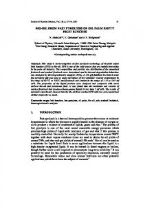
where yt denote observed values of time series (targets) and yˆ t fitted values of time series (outputs). FNN are highly non-parsimonious requiring an infinite amount of past observations as inputs (since an MA can be expressed as an infinite AR) to achieve the same accuracy in forecasting comparing to RNN. Moreover, in practical applications, recurrent neural networks provide a significantly better prediction than a feed-forward network. Figure 1 presents FNN and RNN with a single hidden layer representing nonlinear AR(p) and ARMA(p,q) models, respectively.
GARCH based artificial neural networks in forecasting conditional variance of stock returns Feed-forward neural network with a single hidden layer representing a nonlinear AR(p) model
335
Recurrent neural network with a single hidden layer representing a nonlinear ARMA(p,q) model
yt
yt εˆ t = y t − yˆ t
y t −1
yt − 2 ........ yt − p
y t −1
yt −2 ........ yt − p
εˆt −1 .... εˆt −q
Figure 1 a) FNN with a single hidden layer representing a nonlinear AR(p) model; b) RNN with a single hidden layer representing a nonlinear ARMA(p,q) model
Recurrent neural networks (RNN) are useful, among others, in situations when nonlinear time dependence of financial time series exists. They are constructed by taking a feedforward network and adding feedback connections to previous layers. The standard backpropagation algorithm also trains these networks except that patterns must always be presented in time sequential order. The one difference in the structure is that there is an extra neuron next to the input layer that is connected to the hidden layer just like the other input neurons. This extra neuron holds the contents of one of the layers as it existed when the previous pattern was trained. In this way, the network sees previous knowledge it has about previous inputs. This extra neuron is called the context unit and it represents the network’s long-term memory [2]. The structure of RNN representing nonlinear ARMA(p,q) is comparable to the GARCH(p,q) model with appropriate lag selection. This kind of network is known as the Jordan neural network (JNN). There are two types of RNN: Elman and Jordan recurrent networks. An Elman neural network (ENN) has an additional neuron in the input layer, which is fed back from the hidden layer. However, the ENN does not have an econometric application. A Jordan neural network (JNN) has a feedback connection from the output layer to the input layer. The input layer has an additional neuron, which is fed back from the output layer. Econometric interpretation of such feedback connection lies in the fact that in this way the model is expanded by the lagged error term, i.e., by ε t −i (Figure 1.b). Using JNN the problem of overfitting can
be solved by a more parsimonious model. Although this network is more complicated than a multi-layer feed-forward network, the characteristics of
336
Josip Arnerić, Tea Poklepović and Zdravka Aljinović
feeding back data to the network are similar to the GARCH model, having the previous variance in current forecasts [4]. In general, JNN can be represented as q p (4) yˆ t = f fco + ∑ f ho g fch + ∑ fih yt −i + f rh εˆt −1 , h i 1 1 = = where t is a time index, yˆ t is the output vector, yt −i is the input matrix with
t-i time lags, f(·) and g(·) are activation functions (usually linear and logistic, respectively). φco denotes the constant term in the output layer, φch denotes the constant term in the hidden layer. The weights
φih and φho denote the
weights for the connections between the inputs and hidden neurons and between the hidden neurons and the output, φrh denotes the weight for connections between the context unit and hidden neurons and εˆt −1 denotes the difference
between observed values of time series (targets) and fitted values of time series (outputs) from the previous period. JNN with p inputs, q hidden neurons and one target unit has the abbreviation JNN(p,q,1) [2]. To define appropriate JNN based on GARCH innovations we concentrate on a nonlinear version of ARMA(1,1) originated from equation (4):
εˆt2 = f (α 0 + α1 g (β 0 + β1ε t2−1 + λvˆt −1 ))
(5)
vˆt −1 = ε t2−1 − εˆt2−1
In equation (5), function f (⋅) is the linear activation function in the output layer and g (⋅) is a nonlinear activation function in the hidden layer, which processes information from the input layer to the output layer. A recurrent neural network in (5) assumes one neuron in a single hidden layer network, a nonlinear activation function in a hidden layer, i.e., a sigmoid, a linear activation function in the output layer, one input (squared innovations with one time lag, i.e., ε t2−1 ), one target (current squared innovations, i.e., ε t2 ), while the error term vt is added through feed-back connection from the output layer to the input layer. The parameters α 1 , β1 and λ are the called weights, while
α 0 and β 0 are the biases (constant terms) of the hidden layer and output
layer, respectively. These parameters are estimated from a training sample by minimizing the sum of the squares residuals of innovations
∑ (ε T
t =1
2 t
− εˆt2
)
2
using
the gradient descent procedure known as “backpropagation” (BP). Parameter α 1 is the weight for the connection between the hidden neuron and the output, β1 is the weight for the connection between the input and the hidden neuron, while λ is the “memory weight”. The network, which takes into account all assumptions above, can be presented as a Jordan neural network with memory.
GARCH based artificial neural networks in forecasting conditional variance of stock returns
337
A Jordan net without memory “remembers” only the output from the previous time step. A Jordan net with memory remembers past values as an exponentially decaying weighted average of inputs (no outputs are forgotten; they just “fade away”). The context unit is called a long-term memory unit in a RNN since it remembers past events. According to equation (4), there is only one context unit which accounts for a moving average structure of a time series.
4. Research methodology and results The data set consists of returns of the CROBEX index daily closing prices obtained from the Zagreb Stock Exchange in the period from January 2011 until September 2014. However, for the purpose of this research, the sample is divided into two parts: the in-the-sample part consists of 666 observations in the period from January 2011 until September 2013 which is used for the estimation of parameters in the GARCH(1,1) and the JNN(1,1,1) model; and the out-of-thesample part which consists of the remaining 252 observations, i.e., from September 2013 until September 2014, which is used for the prediction purposes. In order to estimate the JNN(1,1,1) model, in-the sample log returns of the CROBEX index daily closing prices (Figure 1.a) are used for the calculation of squared mean corrected returns (Figure 1.b), i.e., squared innovations which are then used as a target in the JNN. The input for JNN is squared mean corrected returns with one time lag.
Figure 2 a) Daily returns; b) Squared mean-corrected returns
JNN is estimated in R package using the BP algorithm with a constant learning rate. The learning rate is used to update the weights (parameters). When the learning rate is too large, the network may quickly converge to suboptimal local minima. Therefore, an appropriate learning rate should be chosen from the interval [0,1]. In this paper, the learning rate is set to 0.2 to prevent the algorithm from getting stuck in local minima.
338
Josip Arnerić, Tea Poklepović and Zdravka Aljinović
Moreover, with everything else being equal, in this paper 25 JNN (1,1,1) have been estimated only by changing the ratios for the train and the test sample and the weight of the context unit representing the memory of the network. The results of the estimated 25 JNN(1,1,1) are presented in Table 1. Mean squared errors (MSE) are calculated and presented for the train and the test period, and for the out-of-sample period. Moreover, Akaike Information Criteria (AIC) is calculated and presented for the train and the test period, and since it shows divergent results, AIC is averaged.
λ 0.1
0.3
0.5
0.7
0.9
0.1
0.3
0.5
0.7
0.9
train/test MSE(train) MSE(test) MSE(out-of-sample) MSE(train) MSE(test) MSE(out-of-sample) MSE(train) MSE(test) MSE(out-of-sample) MSE(train) MSE(test) MSE(out-of-sample) MSE(train) MSE(test) MSE(out-of-sample) train/test AIC (train) AIC (test) AIC (average) AIC (train) AIC (test) AIC (average) AIC (train) AIC (test) AIC (average) AIC (train) AIC (test) AIC (average) AIC (train) AIC (test) AIC (average)
50%/50% 6.460E-08 6.460E-08 6.315E-08 6.504E-08 6.504E-08 6.412E-08 6.298E-08 6.298E-08 6.312E-08 5.573E-08 5.573E-08 5.531E-08 5.462E-08 5.462E-08 5.312E-08 50%/50% -5502.83 -5502.83 -5502.83 -5500.57 -5500.57 -5500.57 -5511.29 -5511.29 -5511.29 -5552.01 -5552.01 -5552.01 -5558.71 -5558.71 -5558.71
60%/40% 1.589E-09 1.589E-09 1.480E-09 1.539E-09 1.539E-09 1.618E-09 1.521E-09 1.521E-09 1.684E-09 1.702E-09 1.702E-09 1.751E-09 1.536E-09 1.536E-09 1.628E-09 60%/40% -8073.8 -5399.46 -6736.63 -8086.56 -5408 -6747.28 -8091.26 -5411.14 -6751.2 -8046.39 -5381.12 -6713.76 -8087.34 -5408.52 -6747.93
70%/30% 7.441E-10 7.440E-10 8.256E-10 7.470E-10 7.470E-10 6.903E-10 7.978E-10 7.978E-10 8.003E-10 8.008E-10 8.008E-10 6.847E-10 7.420E-10 7.420E-10 7.979E-10 70%/30% -9784.78 -4193.8 -6989.29 -9782.97 -4192.99 -6987.98 -9752.31 -4179.83 -6966.07 -9750.56 -4179.08 -6964.82 -9786.1 -4194.33 -6990.22
80%/20% 1.438E-08 1.438E-08 1.508E-08 1.913E-08 1.913E-08 1.894E-08 1.593E-08 1.593E-08 1.565E-08 1.293E-08 1.293E-08 1.242E-08 1.697E-08 1.697E-08 1.676E-08 80%/20% -9596.55 -2409.7 -6003.12 -9444.71 -2371.45 -5908.08 -9542.09 -2395.98 -5969.04 -9653.1 -2423.94 -6038.52 -9508.45 -2387.5 -5947.98
90%/10% 1.763E-09 1.763E-09 1.611E-09 3.033E-09 3.033E-09 3.323E-09 2.978E-09 2.978E-09 2.797E-09 2.486E-09 2.486E-09 2.692E-09 2.490E-09 2.490E-09 2.687E-09 90%/10% -12063.6 -1340.47 -6702.03 -11738.6 -1304.12 -6521.37 -11749.6 -1305.34 -6527.46 -11857.7 -1317.44 -6587.59 -11856.8 -1317.34 -6587.06
Table 1 MSE and AIC obtained from various JNN(1,1,1) regarding different weights on context unit ( λ ) and a different train/test ratio.
GARCH based artificial neural networks in forecasting conditional variance of stock returns
339
The table shows that MSE firstly decreases with the increase in the train sample, and it is the lowest when 70% of the sample is used for training and 30% for testing, and then it increases. Moreover, it is the lowest when the weight of the context unit λ is the highest, i.e., 0.9. This indicates the longterm memory of this network. When calculating AIC for each network train and test sample, AIC shows extremely divergent results because AIC penalizes for the number of observations and the number of parameters in the model. Therefore, when presenting the average AIC for each network, the results confirm the MSE’s choice of the appropriate NN. Therefore, one neural network is selected based on the lowest MSE and AIC, with 70% of the training and 30% of the testing sample, and with λ equal to 0.9. Results are obtained using the RSNNS package (R – Stuttgart Neural Network Simulator), where the number of units equals 4, and therefore, the number of connections equals 5. The learning rate is set to 0.2 and the learning function is the back-propagation algorithm (JE_BP). The results are presented in Table 2. Input1 Hidden1 Output1 Context1
Input1 0 0 0 0
Hidden1 0.73366 0 0 0.97964
Output1 0 0.00005 0 0
Table 2 Weight matrix for estimated JNN(1,1,1) with ratio 70%/30%.
Context1 0 0 1.0 0.9
λ = 0.9
and the train/test
Although it is obvious that time series is not stationary since the variance of returns is time varying (Figure 2), the CCF (cross-correlation function) test confirmed nonstationarity in variance. Detailed results are omitted due to a lack of space. They are available from authors upon request. Parameters μ
Estimates -0.000111 0.000004* α0 0.075720*** α1 0.853510*** β1 LJ.-B. (1) 4.119 LJ.-B. (2) 4.253 LJ.-B. (5) 5.992 Note: parameter estimates are significant at 1% (***), 5% (**) and 10% (*) significance level using robust standard errors (asymptotic normal and consistent); Ljung-Box (LJ.-B.) test on standardised residuals and standardized squared residuals confirms no serial correlation. Table 3 Estimation of GARCH(1,1) model
340
Josip Arnerić, Tea Poklepović and Zdravka Aljinović
Parameters of the standard GARCH(1,1) model are also estimated using R according to the maximum likelihood method and assuming normal distribution of innovations (rugarch package, i.e., R-Univariate GARCH). These results are given in Table 3. According to parameter estimates, ARMA(1,1) representation of the GARCH(1,1) model can be written as:
εˆt2 = 0.000004 + 0.92923ε t2−1 − 0.85351vˆt −1
(6)
Out-of-sample prediction of the volatility using JNN and GARCH models is presented in Figure 3.
Figure 3 Out-of-sample predictions
The selected JNN(1,1,1) and GARCH(1,1) models are given in Table 4 with their out-of-sample forecasting performances which show superior performances of the neural network model compared to the standard GARCH model. GARCH(1,1)
JNN(1,1,1)
MSE
0.142512
0.121231
RMSE
0.377507
0.348183
Table 4 MSE and RMSE for GARCH(1,1) and JNN(1,1,1) models
GARCH based artificial neural networks in forecasting conditional variance of stock returns
341
5. Concluding remarks Forecasting of volatility, i.e., returns fluctuations, is in the focus of the paper. This research begins with the most widespread approach to volatility modelling, i.e., the GARCH model. Furthermore, ARMA(1,1) representation of the GARCH(1,1) model is defined. However, disadvantages of these models led to an alternative solution, i.e., to define an appropriate neural network which can be analyzed as a nonlinear extension of the ARMA(1,1) model. Therefore, a particular type of RNN, called JNN, is explained in detail and used in further research. Although this network is more complicated than a FNN, the characteristic of feeding back data to the network is similar to the GARCH model, having the previous variance in current forecasts. Therefore, 25 different JNN(1,1,1) have been estimated and the most appropriate network is selected and compared further to the GARCH model. The benefit of using recurrent networks in time series forecasting is reflected in the results, because JNN(1,1,1) presents a better performance than the GARCH(1,1) model in forecasting volatility. A study that analyzes which models best represent the characteristics of financial time series, or better predict their future behaviour is highly beneficial, because that allows market participants to make decisions based on predicted future values. This paper makes contribution in that direction, because it analyzes the performance of the standard GARCH(1,1) model with the performance of the JNN(1,1,1) model in forecasting conditional variance of stock returns on the Croatian stock market. Results of this paper confirm conclusions of previous research about superiority of neural networks versus other linear and nonlinear models. However, they are still a challenge for the researchers in order to improve their performances in forecasting conditional variance of stock returns and time series in general. The use of advanced algorithms in the network training, or other feedback architectures, open space for future work and further studies. Moreover, the limitation of this study can be seen in the pure data. The paper uses only Croatian capital market data, and the market itself is found to be narrow and illiquid. Therefore, future research in this field could be conducted on developed capital markets in order to test the proposed methodology and to obtain results that are more significant. However, the limitation of this paper also presents the challenge for future research since including other countries does not guarantee that the same selected neural network would be most appropriate for all countries.
342
Josip Arnerić, Tea Poklepović and Zdravka Aljinović
Acknowledgments This work has been fully supported by Croatian Science Foundation under the project Volatility measurement, modelling and forecasting (5199).
References [1] Aminian, F., Suarez, E.D., Aminian, M., Walz, D.T. (2006). Forecasting economic data with neural networks, Computational Economics, 28, 71–88. [2] Balkin, S.D. (1997). Using recurrent neural networks for time series forecasting, Working Paper Series number 97–11, International Symposium on Forecasting, Barbados [3] Bollerslev, T. (1986). Generalized autoregressive conditional heteroskedasticity, Journal of Econometrics, 31, 307–327. [4] Dechpichai, P. (2010). Nonlinear neural network for conditional mean and variance forecasts, Doctor of Philosophy thesis, University of Wollongong, School of Mathematics and Applied Statistics, University of Wollongong, Dubai. [5] Donaldson, R.G. and Kamstra, M. (1997). An artificial neural network - GARCH model for international stock return volatility, Journal of Empirical Finance, 4 (1), 17–46. [6] Dunis, C.L., Williams, M. (2002). Modelling and trading the euro/US dollar exchange rate: Do neural networks perform better?, Journal of Derivatives & Hedge Funds, 8, 3, 211–239. [7] Engle, R.F. (1982). Autoregressive conditional heteroskedasticity with estimates of the variance of UK inflation, Econometrica, 41, 135–155. [8] Franses, P.H., van Dijk, D. (2003). Nonlinear Time Series Models in Empirical Finance, Cambridge University Press. [9] Ghiassi, M., Saidane, H., Zimbra, D.K. (2005). A dynamic artificial neural network model for forecasting time series events, International Journal of Forecasting 21, 341–362 [10] Gonzales, S. (2000). Neural networks for macroeconomic forecasting: A complementary approach to linear regression models, Working Paper 2000–07. [11] Hwarng, H.B. (2001). Insights into neural-network forecasting of time series corresponding to ARMA(p,q) structures, Omega 29, 273–289. [12] Kuan, C.-M. and White, H. (2007). Artificial neural networks: An econometric perspective, Econometric Reviews, 13, 1–92 [13] Lamoureux, C. and Lastrapes, W. (1990). Persistence in variance, structural change, and the GARCH model, Journal of Business and Economic Statistics, Vol. 8, 225– 234. [14] Lawrence, S., Giles, C.L., Tsoi, A.C. (1997). Lessons in neural network training: Overfitting may be harder than expected, Proceedings of the Fourteenth National Conference on Artificial Intelligence, AAAI-97, 540–545.
GARCH based artificial neural networks in forecasting conditional variance of stock returns
343
[15] Maillet, B.B. and Merlin, P.M. (2009). Outliers detection, correction of financial time-series anomalies and distributional timing for robust efficient higher-order moment asset allocations (September 16). [16] Mantri, J.K., Gahan, P. and Nayak, B.B. (2010). Artificial neural networks – An application to stock market volatility, International Journal of Engineering Science and Technology, Vol. 2(5), 1451–1460. [17] Mantri, J.K., Mohanty, D. and Nayak, B.B. (2012). Design neural network for stock market volatility: Accuracy measurement, International Journal on Computer Technology & Applications, Vol. 3 (1), 242–250. [18] Sarangi, P. and Dublish, S. (2013). Prediction of gold bullion return using GARCH family and artificial neural network models, Asian Journal of Research in Business Economics and Management Vol. 3, No. 10, 217–230. [19] Tal, B. (2003). Background information on our neural network-based system of leading indicators, CBIC World Markets, Economics & Strategy, September [20] Täppinen, J. (1998). Interest rate forecasting with neural networks, Government Institute for Economic Research, Vatt-Discussion Papers, 170. [21] Visković, J., Arnerić, J. and Rozga, A. (2014). Volatility switching between two regimes. World Academy of Science, Engineering and Technology, International Science Index 87, International Journal of Social, Management, Economics and Business Engineering, 8(3), 682–686. [22] Wong, C.S. and Li, W.K. (2001). On a mixture autoregressive conditional heteroscedastic model, Journal of American Statistical Association, Vol. 96, No. 455, 982–995. [23] Zekić-Sušac, M. and Kliček, B. (2002). A nonlinear strategy of selecting NN architectures for stock return predictions, Finance, Proceedings from the 50th Anniversary Financial Conference Svishtov, Bulgaria, 11–12 April, Svishtov, Veliko Tarnovo, Bulgaria: ABAGAR, 325–355. [24] Zhang, G.P. (2003). Time series forecasting using hybrid ARIMA and neural network model, Neurocomputing 50, 159–175.