A distributed modular logic programming model based on the cortex Alan H. Bond 1
Semel Institute for Neuroscience, Geffen Medical School, University of California at Los Angeles, Los Angeles, California 90095 and 2 National Institute of Standards and Technology, MS 8263, Gaithersburg, Maryland 20899
[email protected], http://www.exso.com
Abstract. We developed a distributed modular architecture based on distribution of processing and storage according to data type, inspired by an analysis of the primate cortex. Data items and rules have sets of weights, and these are updated, attenuated and combined in various ways to allow data storage management and rule competition. There are many motivations for using weights, including modeling strengths of different primate behaviors, storage management so that data items are stored and removed from store as needed, rule selection by competition based on computed weight, rule selection stability by confirmation feedback among modules, time smearing to prevent propagation delay problems within the distributed architecture, and the desire to eventually find corresponding neural models.
1
Motivation from neuroscience
We used a modeling approach of a modular distributed computational architecture and an abstract logical description of data and control [1] [2] [5], for which we have also analyzed the correspondence to the primate neocortex [6]. We analyzed the neuroanatomy of the cortex, which is divided into neural areas with genetically determined connections among areas [6]. We reviewed experiments which indicated the functions that each neural area appeared to be involved in, and we construed these results as each neural area’s action being to construct data items of data types characteristic of that area. We also defined neural regions made up of small numbers of areas, as there are about 50 cortical areas whose functions are sometimes not clearly differentiated. The end result of our analysis is summarized in Figure 1. In order to design a model of the cortex, we abstracted from our review some biological information-processing principles: 1. Each neural area stores and processes data items of given types characteristic of that neural area; data items are of bounded size. 2. To form systems, neural areas are connected in a fixed network with dedicated point-to-point channels. 3. The set of neural areas is organized as a perception-action hierarchy.
G
MI muscle SI combinations tactile detection PA3 specific plans PA4 complex plans
PA1 detailed actions
PA5 contexts and episodes
PA4
DV1
maps DV3 social SS3 visual SS2 soc SS1 tactiletact.feat. tactile guid.feat. images
PA2 eye saccades
PA5
DV2
AU2 social messages
PA2
PA1
MI
SS3
SS2
SS1
SI
DV3
DV2
DV1
AU2
AU1
DV1 spatial features
AU3
G goals
PA3
AI PM1 auditorysocial detection action features AU1 auditory VV1 features PM2 social object action identities features
AI
VI visual features
PM3
PM3 social AU3 goal social messages features
VV3
VV2 complex and VV3 episodic social objects memory
(a)
PM2
PM1
VV2
VV1
VI
OL1
OI
GU1
GI
(b)
Fig. 1. (a) Lateral view of the cortex showing neural regions and functional involvements, (b) Connectivity of regions showing perception-action hierarchy
4. Neural areas process data received and/or stored locally by them. There is no central manager or controller. 5. All neural areas have a common execution process, the “uniform process”, which constructs data items. 6. All neural areas do similar amounts of processing and run at about the same speed. 7. There is data parallelism in communication, storage and processing. Processing within a neural area is highly parallel. Parallel coded data is transmitted, stored, and triggers processing. Processing acts on parallel data to produce parallel data. 8. The data items being transmitted, stored and processed can involve a lot of information; they can be complex. 9. The set of neural areas acts continuously and in parallel. From these and other considerations which we will explain, we designed and implemented a model of the cortex [2] [5].
2
Summary of our modeling approach
In the last few years, we have conducted a series of studies and models concerning the human brain, including problem solving [4], episodic memory [8], natural language processing [7], routinization [9], and social relationships [3]. We used Sicstus Prolog as a basic implementation language and added another layer which we called BAD, Brain Architecture Description language, which represented the parallel execution of modules and communication channels between modules. 2
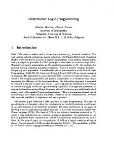
A system-level brain model is a set of parallel modules with fixed interconnectivity similar to the cortex, and where each module corresponds to a brain area and processes only certain kinds of data specific to that module. We view all data streams and storage as made up of discrete data items which we call descriptions. We represent each data item by a logical literal which indicates the meaning of the information contained in the data item. An example data item is position(adam,300,200,0) which might mean that the perceived position of a given other agent, identified by the name “adam”, is given by (x,y,z) coordinates (300,200,0). In order to allow for ramping up and attenuation effects, we give every data item an associated strength, which is a real number. Stored data items are ramped up by incoming identical or related data items, and they also attenuate with time, at rates characteristic of the module and data type. We represent the processing within a module by a set of left-to-right logical rules. Our logical rules are clauses, i.e., they have no nesting, but are made up of a disjunction of literals, which are executed in parallel. A rule matches to incoming transmitted data items and to locally stored data items, and generates results which are data items which may be stored locally or transmitted. Rule patterns also have weights, and the strength of a rule instance is the product of the matching data item weights and the rule pattern weights, multiplied by an overall rule weight. A rule may do some computation which we represent by arithmetic and conditionals. This should not be more complex than can be expected of a neural net. The results are then filtered competitively depending on the data type. Typically, only the one strongest rule instance is allowed to “express itself”, by sending its constructed data items to other modules and/or to be stored locally. In some cases however all the computed data items are allowed through. The system works on a discrete time scale, in cycles. Each cycle is identified with a period of 20 milliseconds, since this is the characteristic time found in the primate brain for processing of data in one area and transmitting it to another adjacent area. Thus, we expect computation at the level of individual rule firings to be fairly fine grained in terms of the application area. Also, within each cycle, all possible instances of all rules are executed and then the results compete to determine which of them will update the store of the module and which will be output to other modules. In one cycle, all rules are repeatedly executed until there is no change in the store. During this process, only the updates are stored, until stability, then the outputs are made. This repetition, or iteration, is done to ensure integrity of the store before any communication with other modules. The uniform process of the cortex is then the mechanism for storage and transmission of data and the mechanism for execution of rules. Modules are organized as a perception-action hierarchy, which is an abstraction hierarchy with a fixed number of levels of abstraction. Our approach is intended to be complementary to neural network approaches, and it should be possible, for a given abstract model, to construct corresponding neural network models. Figure 2 diagrams our initial model, and Figure 3 shows an example scenario 3
MI muscle combinations PA1 detailed actions for self
SI tactile detection SA1 tactile images
DV2 spatial maps
PA3 specific joint plans and plan persons
DV1 spatial features
PA4 overall plans
PM1 person positions and movements
G goals
PM2 person actions and relations
VI visual features
VV1 object identities
PM3 social dispositions and affiliations
tactile input
motor output
visual input
Fig. 2. Outline diagram of an initial model
which determines the external input and output descriptions used by the model. This example has two modeled brains, one for each primate.
3 3.1
Data, storage and processing within modules Data items
A brain (or brain subsystem) is described by an interconnected set of processing modules. Each module contains data of only given types. All data items are represented by descriptions. To indicate what data types can be stored in a given module, for each data type we give a description pattern, which defines a set of descriptions consisting of all of its instances. Currently, all description patterns are literals of the form: predicate([C,W1,W2,Time stamp,Rstate],Context,[List of values]) (using initial capitals to indicate variables). The Context term is intended to be used for grouping descriptions into sets, i.e., all those descriptions with the same value of Context form a set. C is a certainty factor and W1 and W2 are weights; all of these are reals. In List of values, all values are ground terms, preferably atomic. An example of a description pattern is position(W,C,[Agent,X,Y,Z]), which might be a data type whose instances represent the position X,Y,Z of a perceived Agent, with certain weights. An example of a description, i.e. data item, is a substitution instance of this data type: position([1.0,1.0,1.0,1,[]],any,[adam,300.0,200.0,0.000]) 4
Fig. 3. Example of modeled primate behavior
At any one time, the module store has a set of stored descriptions of given types. A specification of a description type also includes its updating properties, its competition characteristics and its rates of update and attenuation, which will be explained below. 3.2
Rules
Computation in modules is represented by a set of description transformation rules of the form: rule(agent,rule_name,context, if((sequence of description patterns)), then ([list of description patterns]), provided((clause_body)), weights(weights)). It is executed by matching the left hand side to bind variables and then constructing and possibly storing the descriptions given by the right hand side. For example: rule(M,macroaction_2,context(all), 5
if((position(W,C,[M,X,Y,Z]), position(W_p,C,[MP,XP,YP,ZP]))), then([near(W_1,any,[M,MP])],Wa), provided((MP \== M, distance(X,Y,Z,XP,YP,ZP,D),D 100.0,!,fail) | true), which, if the variable Agent does not occur in the left-hand side of the rule, means there does not exist any agent with Z > 100.0. If Agent does occur in the left-hand side of the rule then this is equivalent to having a pattern position(W,C,[Agent,X,Y,Z]) in the left hand side and a test Z > 100.0 in the body of the rule. 3.5
Competition
All descriptions and all rule activations have a weight which is a number representing their strength. The simplest form of competition is just to compare the weights of all the rule instances and to select just the strongest one. The products of this one rule are then stored and/or transmitted. However, we have found it useful, and necessary, to develop other forms of competition, as follows. Those product literals which are to update the store we call updates and those which are to be transmitted to other modules we call outputs. All the updates and outputs generated by the set of rule executions in a given time cycle are subjected to competition as specified by the user in list of rule number sets, update patterns and output patterns. Here is how rule competition is specified: list of rule number sets(M,Mod,[list of lists of rule numbers]). Results from all the rule instances from rule numbers in each set compete against each other. The results of a rule comprises the instantiated right hand side and the Wa value which is the overall rule instance strength. Rule competition uses just the Wa values. For example, list of rule number sets(M,Mod,[[R1,R2],[R3,R5]]))). which defines a list of rule number sets e.g. [R1,R2],[R3,R5]. Then all the results from rules R1 and R2 have their Wa values compared and only the one with the largest Wa is used. The same for R3 and R5. Results from any other rules all go through and are used. Thus there is first competition among entire rules, and then competition among all the individual constructed literals. This is necessary or else it would be possible for one literal from one rule and one from another to succeed, but other literals from the same rules to fail. In general, for rule competition, we are thinking of changing to using rule priority ordering, that is, each rule having a place in a, possibly partial, ordering which determines its dominance in competition, independently of computed strengths. Such an ordering could be dynamic. This would give a more stable method, with better expressive discrimination, than using weights. After rule competition, all the surviving updates and outputs from the rule instances are made into two overall lists. These lists, of updates and outputs respectively, are then, if desired, subjected to individual competition among descriptions in the list. 7
The way update competition currently works is as follows: for each pattern in a specified list of update patterns, all the generated descriptions which match to that pattern are compared and only the one with the largest W1 weight is allowed to actually update the store. In addition, the winning W1 weight must be greater than a specified threshold. Any generated updates which do not match any update pattern are allowed to update the store. The analogous method is used for outputs also.
3.6
Storage of data, uniqueness, similarity and novelty
When we implemented and ran our model we soon realized that the store was updated from inputs every cycle and these updates were often very similar to those of the previous cycles. In order to update the store, we had to test if the input literal was the same as an existing stored literal. In fact there were four cases (1) input literal identical to a stored one, including all the weights, (2) the input literal is the “same” as a stored one, i.e. only differing in the values of the weights, (3) “similar”, which is given by equivalence expressions so that a data item may overwrite a “similar” one already in the store, for example if the action is walking and then the next input has it standing, we update the stored one, even though it is not the “same” as defined above, (4) the input literal is “novel” meaning it is not identical, same or similar, in which case it is simply stored. We also have sometimes used “comparable”, based on X,Y,Z nearness. In addition, we found we had to specify update characteristics for each data type; we used memory item update characteristic patterns, or item types: items matching these patterns replace existing items: item type(Person,Module,Type,[Input pattern,Stored pattern]). An incoming description is matched to the Input pattern, if it matches, then the Stored pattern is matched to the store. If this matches then the incoming description updates the matching stored description. If no Input pattern matches, or if the Stored pattern does not match to the store then the description is simply stored, as it is a novel item. e.g., item type(Person,Module,data,[goal(G),goal(G)]). any incoming goal description updates only an identical one. Thus there can be an indefinite number of goal descriptions, with different goals G. e.g., item type(Person,Module,data,[action(M1,A1),action(M1,A2)]). an incoming action description for a given person M1 updates any other action description for the same person. Thus, only one action description can exist for a given person, however there can be an indefinite number of different action descriptions each for a different person. The updating of weights of memory items from incoming weights of matching item uses a multiplicative linear increment to the excitation of the item: update weights increment(Person,Module,Incw1,Incw2). (((W1 input >= W1 old),W1 new is (W1 old*(1.0 + Incw1))) | ((W1 input < W1 old),W1 new is (W1 old*(1.0 - Incw2)))). 8
3.7
Attenuation
All stored data items are subject to an exponential attenuation process each cycle. Attenuation reduces the weight by a standard fraction each cycle. This fraction can be set to zero so there is no attenuation, and it can also be set to one, which erases the data item after one cycle (not before it contributes to rule matching in the cycle). Thus, attenuation factors are specified: attenuation factor input(Person,Module,Type,DW,Description pattern). e.g. for data to attenuate to noise level in about 20 cycles attenuation factors(Person,Module,data,[0.1,0.1,0.1],C) Noise level can be set and is the value at which a description is removed from the store: noise level(Person,Module,Type,Noise level). As a result of continuous linear updating and exponential attenuation, with a constant input stream of data items, the stored value will settle to a steady value. Initially, there will be a build up of the weight taking a few cycles, starting from noise level, and when the input ceases or changes to some other data items, the weight will take a few cycles to attenuate to noise level, where it is then deleted. 3.8
The rule execution regime
During each such processing cycle, each module is processed once. 1. all input descriptions on input channels from other modules are stored by updating into the module 2. all instances of all rules are executed 3. all generated updates are subjected to competition 4. all winning updates are used to update the store of the module 5. all generated outputs are subjected to competition 6. all winning output descriptions are transmitted to output channels to other modules. Since the rules are independent it doesn’t matter what order they are processed in. This is equivalent to complete parallelism of the system, at the level of the modeling abstraction being used here. 3.9
Other uses of weights
Certainty and primate behavior. Initially, we developed a model of the primate cortex and the first behavior we modeled was grooming of one primate by another. In nature, primates will not groom unless and until they have established a relationship of dominance and submission with an acceptable degree of certainty. Grooming then maintains a certain relationship strength. We assumed that the memory of these certainties and strengths tended to attenuate and were maintained by dominance-determining behaviors and relationship-strengthening behaviors. Thus when certainty of the assessed dominance between two primates fell below a threshold, the primates would challenge each other, and depending on the results of this, would renew the dominance relationship. Similarly when 9
relationship strength fell below threshold, a goal to groom was created leading to grooming behavior until the strength had increased enough. Time smearing. We found that, without these mechanisms, the distributed system could fail to establish intended patterns of activation because of the time delay in data changes being created in one module and arriving at another module several steps away. Thus a plan step could be constructed a couple of cycles before data arrived specifying the coordinates to use, leading to the plan step failing and another being tried. Using weights tended to smear these times and allow different data streams to combine successfully.
4
Conditional elaboration, sequencing, abstraction levels, attention
As we indicated above, the modules are arranged in a perception-action hierarchy. A schematic diagram of our concept of perception-action hierarchy is given in Figure 4. memory of social relations
observations of social relations
goals received from system
disposition relative to goals
goals prioritized and selected goal sent evaluation requests for information on goals and dispositions
perception of goals and dispositions
joint plan selected
requested information perception
perception in terms of relations ; attention dependent on information received
attention requests for information on actors and actions
evaluation
elaboration joint plan described in relational terms; elaboration conditional on relational information received
requested information perception
perception of spatial detail ; attention dependent on information received
attention evaluation requests for information on spatial positions etc
elaboration
requested information attention
perception
evaluation
plan for self described in spatial detail ; elaboration conditional on geometric information received elaboration generation of detailed motor commands
perception of features
from sensors
to effectors
Fig. 4. The mechanisms of a perception-action hierarchy
10
Modules are arranged in a hierarchy of abstraction. The system elaborates a selected goal into a plan and then into a succession of more detailed plans until finally a concrete action for the next cycle is sent to effectors which act on the environment. We made the effector output a motor goal which was renewed every cycle. We made the top level of plan description correspond to social plans, which specified, in each plan step, not only the action of the agent but also the expected perceived action(s) of the other interacting agent(s). In executing a social plan, the perceived behavior of the other interacting agents was first checked to ensure it was in agreement with the currently executed social plan, and also to extract matched variable values for use in constructing the agent’s own actions. An example of a social plan is approaching and shaking the hand of another person. Plan elaboration is depicted in Figure 5. At each level the currently selected plan element is computed, so all levels continuously compute in parallel. This affiliation(adam1,alice1,0.6,0.8) dominates(alice1,adam1,0.8) rule generates affiliation goal
social relations module
goal(affiliate(adam1,alice1)) goal(affiliate(adam1,alice1)) rule calculates goal’s priority disposition(goal(affiliate( adam1,alice1)),positive,0.7)
goals module
goal(affiliate(adam1,alice1)) goal(affiliate(adam1,alice1)) overall plans module plan(groom(X,Y)) rule selects joint plan and instantiates it plan(groom(adam1,alice1))
orienting_towards(alice1,adam1)
plan(groom(adam1,alice1)) rule constructs detailed joint action step
specific joint plans module
plan_self(approach(alice1)) position(alice1,300,200,0)
plan_self(approach(alice1)) rule constructs detailed action for self
detailed actions for self module
self_act(move_to(300,200,0))
Fig. 5. Parallel elaboration
arrangement will also allow us to model episodic thinking as described by Newell and Simon [11], and also by DeGroot [10] for chess thinking. The interaction of the perception and action hierarchies results in conditional elaboration and attention mechanisms, see Figure 6. By conditional elaboration, we mean that the current percept can modify the elaborated plan step, so for example the agent can track and act upon a changing environment. By attention, we mean that information from plan elaboration is passed to the perception hierarchy and can modify the use of perceptual resources to process in more detail the objects or other agents that the agent is interacting with. 11
description of goal goal groom(alice1) spatial relations
far(alice1)
groom(M1),near(M) −> prelude(M1) groom(M1),far(M1),oriented(M,M1) −> approach(M1) approach(alice)
detailed positions
position(alice,50,40,0)
description of action in terms of spatial relations
approach(alice) approach(M),position(M,X,Y,Z)−>move_to(X,Y,Z) move_to(50,40,0)
goal and relational information generate action description
action description and detailed position generate detailed action
description in terms of coordinates
(a) conditional elaboration
groom(alice) attend(alice)
attend(M), check_near(M)
too_near(alice) if too_near(M) etc.
(b) attention
action concerns alice module sends attend(alice) data item to perceptual module action module receives detailed perceptual information about alice
Fig. 6. Conditional elaboration and attention
Hierarchy of timing. We found that characteristic times for volatility of data were best organized hierarchically, so that nearer the periphery, either sensors or effectors, we had faster timing, typically setting attenuation to 100%. Otherwise the previous values would cause thrashing of various types, in the motor case producing motor problems reminiscent of those observed in people with different forms of ataxia.
5 5.1
Confirmation and viable states Confirmation
In order to select rules which were successful in producing useful behavior, we developed a mechanism which we call confirmation. If a rule fires in one “source” module and sends a description to another “target” module, then if this causes some rule in the target module to fire then a confirmation message is sent back to the source module. This message is specific to the exact description originally sent, see Figure 7. Thus there is no need for global evaluation, and the test is purely local to the target module. The rule instance in the source module then has its value boosted by the confirmatory message. This will tend to keep it in control and keep things stable, avoiding “jitter”. If on the other hand no rule in the target module is caused to fire, then the rule instance is disconfirmed which results in it being placed in a “refractory” state for a certain period of time. This allows other competing rule instances to be tried. The general idea is that 12
the system will then try all the different rule instances until it finds one that makes something happen, so this is a little like backtracking but with a simpler mechanism.
friend(alice1) friend(alice2) should_affiliate(alice1) should_affiliate(alice2) friend(M1),should_affiliate(M1) −> affiliate(M1) affiliate(alice2)
rule fires for both alice1 and alice2 rule instance for alice2 is strengthened by confirmation
confirm(affiliate(alice2)) affiliate(alice1) is not confirmed affilate(alice2) is confirmed
near(alice2) affiliate(alice1) affiliate(alice2) near(M1),affiliate(M1) −> groom(M1)
groom(alice2)
Fig. 7. Confirmation
The way this is actually implemented is to not send any message in the disconfirmation case, so the source module simply waits a certain number of cycles before timing out and disconfirming the currently active rule instance. Thus, we keep time stamps stored in each literal which give its waiting state and its refractory state, and the attenuation mechanism updates these each cycle. Thus data items are actually time-dependent literals. Confirm factors specify the impact of confirmation values on weights: confirm factors(Person,Module,Type,[CFNEG,CFPOS], [Confirm threshold,CSNEG,CSPOS]) where: (i) Confirm threshold determines where the computed confirmation value is a positive or negative confirmation (ii) CFNEG is subtracted from W1 for negative, i.e. dis-, confirmation and (iii) CFPOS is used to multiply the confirmation value that is added to W1 for positive confirmation. Typical values are e.g. confirm factors(M,goal,data,[0.4,0.05],[0.2,1.0,1.0]). 5.2
Viable states
A system will tend to transition into what we call a viable state, in which the perceived environment tends to support the selected plan and the plan is selected by and supports the currently selected goal. Thus, in a viable state, the agent carries out a planned action which is relevant to its current goals, and which can be successfully carried out in the current external environment. The idea of a viable state is depicted in Figure 8. In each module, there is a dominant rule which fires and wins the competition with other rule instances. The other rule instances continue to be computed each cycle. 13
affiliation
goal
person_disposition
plan
plan_person
plan_person_action
person_action
person_motion
plan_self_action
sensor_system
motor_system environment
Fig. 8. The idea of a viable state
Once in a viable state the system will tend to stay in it for several cycles, a few tens of cycles, up to thousands of cycles, before it has to select a new plan step at some level and to transition into another viable state. During a transition period, modules try different rules until they find one that is confirmed, and then until all the modules are selecting rules which are confirmed. It usually takes about 10 to 15 cycles to establish the next viable state, which corresponds to the observed time of 300 milliseconds to establish a conscious state. Multiple interacting agents will also find mutually viable states, where the perceived behaviors of the other agents are compatible with the social plans being executed by each agent.
6
Summary and conclusion
We have developed a biologically-inspired modular distributed model based on distribution of storage and processing according to data type. Real-valued weights on data and rules were used for several disparate purposes in this system, as a result of different requirements and problems, namely: to model certainties in primate behavior, to provide time smearing and better coordination 14
and architectural coherence within the distributed system, for competitive rule selection, for rule stabilization by confirmation or temporary deselection by disconfirmation, for storage management, allowing older data non-refreshed to be removed, and for the future development of mapping to neural net models.
References 1. Alan H. Bond. A Computational Architecture for Social Agents. In Proceedings of Intelligent Systems: A Semiotic Perspective, An International Multidisciplinary Conference, National Institute of Standards and Technology, Gaithersburg, Maryland, USA, Oct 20-23, 1996. 2. Alan H. Bond. Describing Behavioral States using a System Model of the Primate Brain. American Journal of Primatology, 49:315–388, 1999. 3. Alan H. Bond. Modeling social relationship: An agent architecture for voluntary mutual control. In Kerstin Dautenhahn, Alan H. Bond, Dolores Canamero, and Bruce Edmonds, editors, Socially Intelligent Agents: Creating relationships with computers and robots, pages 29–36. Kluwer Academic Publishers, Norwell, Massachusetts, 2002. 4. Alan H. Bond. Problem-solving behavior in a system model of the primate neocortex. Neurocomputing, 44-46C:735–742, 2002. 5. Alan H. Bond. A Computational Model for the Primate Neocortex based on its Functional Architecture. Journal of Theoretical Biology, 227:81–102, 2004. 6. Alan H. Bond. An Information-processing Analysis of the Functional Architecture of the Primate Neocortex. Journal of Theoretical Biology, 227:51–79, 2004. 7. Alan H. Bond. A psycholinguistically and neurolinguistically plausible systemlevel model of natural-language syntax processing. Neurocomputing, 65-66:833–841, 2005. 8. Alan H. Bond. Representing episodic memory in a system-level model of the brain. Neurocomputing, 65-66:261–273, 2005. 9. Alan H. Bond. Brain mechanisms for interleaving routine and creative action. Neurocomputing, 69:1348–1353, 2006. 10. Adriaan D. de Groot. Het Denken van den Schaker. North Holland, Amsterdam, 1946. Translation into English and published as Thought and Choice in Chess, Mouton, 1965. 11. Allen Newell and Herbert Simon. Human problem solving. Prentice Hall, Englewood Cliffs, New Jersey, 1972.
15