Jan 26, 2007 - using a Euclidean D3-brane wrapping a 4-cycle inside the resolved ...... 5-cycle was the trivial cycle that could shrink to a point at the place ...
arXiv:hep-th/0701064v2 26 Jan 2007
PUPT-2221 hep-th/0701064
Gauge/Gravity Duality and Warped Resolved Conifold
Igor R. Klebanov and Arvind Murugan Department of Physics and Princeton Center for Theoretical Physics Princeton University, Princeton, NJ 08544
We study supergravity backgrounds encoded through the gauge/string correspondence by the SU(N)× SU(N) theory arising on N D3-branes on the conifold. As discussed in hep-th/9905104, the dynamics of this theory describes warped versions of both the singular and the resolved conifolds through different (symmetry breaking) vacua. We construct these supergravity solutions explicitly and match them with the gauge theory with different sets of vacuum expectation values of the bi-fundamental fields A1 , A2 , B1 , B2 . For the resolved conifold, we find a non-singular SU(2) × U(1) × U(1) symmetric warped solution produced by a stack of D3-branes localized at a point on the blown-up 2-sphere. It describes a smooth RG flow from AdS5 × T 1,1 in the UV to AdS5 × S 5 in the IR, produced by giving a VEV to just one field, e.g. B2 . The presence of a condensate of baryonic operator detB2 is confirmed using a Euclidean D3-brane wrapping a 4-cycle inside the resolved conifold. The Green’s functions on the singular and resolved conifolds are central to our calculations and are discussed in some detail.
1
1 INTRODUCTION
Contents 1 Introduction
1
2 The Conifold and its Resolution
3
3 Flows on the Singular Conifold
5
4 Flows on the Resolved Conifold
8
5 B-field on the Resolved Conifold
14
6 Conclusions
14
A Eigenfunctions of the Scalar Laplacian on T 1,1
15
B AdS5 × S 5 Throats in the IR
18
1
Introduction
The basic AdS/CFT correspondence [1, 2, 3] (see [4, 5] for reviews) is motivated by considering the low energy physics of a heavy stack of D3-branes at a point in flat spacetime. Taking the near-horizon limit of this geometry motivates a duality between type IIB string theory on AdS5 × S 5 and N = 4 SU(N) supersymmetric Yang-Mills gauge theory. This correspondence was generalized to theories with N = 1 superconformal symmetry in [6, 7] by considering a stack D3-branes, not in flat space, but placed at the tip of a 6d Calabi-Yau cone X6 . The near horizon limit in this case turns out to be AdS5 × Y5 where Y5 is the compact 5 dimensional base of X6 and is a Sasaki-Einstein space. Among the simplest of these examples is Y5 = T 1,1 , corresponding X6 being the conifold. It was found that the low-energy gauge theory on the D3-branes at the tip of the conifold is a N = 1 supersymmetric SU(N) × SU(N) gauge theory with bi-fundamental chiral superfields Ai , Bj (i, j = ¯ ) and (N, ¯ N) representations of the gauge groups, respectively [6, 7]. The superpotential 1, 2) in (N, N for this gauge theory is W ∼ Tr det Ai Bj = Tr (A1 B1 A2 B2 − A1 B2 A2 B1 ). The continuous global symmetries of this theory are SU(2) × SU(2) × U(1)R × U(1)B where the SU(2) factors act on Ai and Bj respectively, U(1)B is a baryonic symmetry, and U(1)R is the R-symmetry with RA = RB = 12 . This assignment ensures that W is marginal, and one can also show that the gauge couplings do not run. Hence this theory is superconformal for all values of gauge couplings and superpotential coupling [6, 7]. When the above gauge theory is considered with no vacuum expectation values (VEV’s) for any of the fields, we have a superconformal theory with the AdS5 × T 1,1 dual. In [8], more general vacua of this theory were studied. It was argued that moving the D3-branes off the tip of the singular conifold corresponds to a symmetry breaking in the gauge theory due to VEV’s for the A, B matter fields such that the VEV of operator U=
� 1 Tr |B1 |2 + |B2 |2 − |A1 |2 − |A2 |2 N
(1)
vanishes. Further, more general vacua exist for this theory in which this operator acquires a non-zero
1 INTRODUCTION
2
VEV.1 It was pointed out in [8] that these vacua cannot correspond to D3-branes on the singular conifold. Instead, such vacua with U = 6 0 correspond to D3-branes on the resolved conifold. This “small resolution” is a motion along the K¨ahler moduli space where the singularity of the conifold is replaced by a finite S 2 . Thus the SU(N) × SU(N) gauge theory was argued to incorporate in its different vacua both the singular and resolved conifolds. On the other hand, the deformation of the conifold, which is a motion along the complex structure moduli space, can be achieved through replacing the gauge theory by the cascading SU(N) × SU(N + M) gauge theory (see [9]). One of the goals of this paper is to construct the warped SUGRA solutions corresponding to the gauge theory vacua with U = 6 0. Our work builds on the earlier resolved conifold solutions constructed by Pando Zayas and Tseytlin [10], where additional simplifying symmetries were sometimes imposed. Such solutions corresponding to D3-branes “smeared” over a region were found to be singular in the IR [10]. We will instead look for “localized” solutions corresponding to the whole D3-brane stack located at one point on the (resolved) conifold. This corresponds to giving VEV’s to the fields Ai , Bj which are proportional to 1N ×N . We construct the duals of these gauge theory vacua and find them to be completely non-singular. The solution acquires a particularly simple form when the stack is placed at the north pole of the blown up 2-sphere at the bottom of the resolved conifold. It corresponds to the simplest way to have U = 6 0 by setting B2 = u1N ×N while keeping A1 = A2 = B1 = 0. Following [11, 8], we also interpret our solutions as having an infinite series of VEV’s for various operators in addition to U. For this, we rely on the relation between normalizable SUGRA modes and gauge theory VEV’s in the AdS/CFT dictionary. When a given asymptotically AdS solution has a (linearized) perturbation that falls off as r −∆ at large r, it corresponds to assigning a VEV for a certain operator O of dimension ∆ in the dual gauge theory [11, 8]. The warp factor produced by a stack of D3-branes on the resolved conifold is related to the Green’s function on the resolved conifold. This warp factor can be expanded in harmonics and corresponds to a series of normalizable fluctuations as above, and hence a series of operators in the gauge theory acquire VEV’s.2 For this purpose, we write the harmonics in a convenient set of variables ai , bj that makes the link with gauge theory operators built from Ai , Bj immediate. Due to these symmetry breaking VEV’s, the gauge theory flows from the SU(N) × SU(N) N = 1 theory in the UV to the SU(N) N = 4 theory in the IR, as one would expect when D3-branes are placed at a smooth point. The SUGRA solution is shown to have two asymptotic AdS regions – an AdS5 × T 1,1 region in the UV, and also an AdS5 × S 5 region produced in the IR by the localized stack of D3-branes. This can be considered an example of holographic RG flow. The Green’s functions determined here might also have applications to models of D-brane inflation, and to computing 1-loop corrections to gauge couplings in gauge theories living on cycles in the geometry [15, 16]. When the branes are placed on the blown up 2-sphere at the bottom of the resolved conifold, this corresponds to A1 = A2 = 0 in the gauge theory. Hence no chiral mesonic operators, such as TrAi Bj , have VEV’s, but baryonic operators, such as det B2 , do acquire VEV’s. Therefore, such solutions, parametrized by the size of the resolution and position of the stack on the 2-sphere, are dual to a “non-mesonic” (or “baryonic”) branch of the SU(N)×SU(N) SCFT (see [17] for a related discussion). These solutions have a blown up S 2 . On the other hand, the solutions dual to the baryonic branch of the cascading SU(N) ×SU(N + M) gauge theory were constructed in [18, 19] (for an earlier linearized 1
As was pointed out in [6], no D-term equation constrains this operator since the U (1) gauge groups decouple in the infrared. 2 In the N = 4 SUSY example, the normalizations of the VEV’s have been matched with the size of the SUGRA perturbations around AdS5 × S 5 (see [12, 13, 14]). In this paper we limit ourselves to a more qualitative picture where the precise normalizations of the VEV’s are not calculated.
2 THE CONIFOLD AND ITS RESOLUTION
3
treatment, see [20]) and have a blown up S 3 supported by the 3-form flux. The paper is organized as follows. In Section 2, we review and establish notation for describing the conifold, its resolution, its symmetries and coordinates that make the symmetries manifest. We also review the metric of the resolved conifold and the singular smeared solution found in [10]. In Section 3, as a warm up, we study the simple example of moving a stack of D3-branes away from the tip of the singular conifold. We present the explicit supergravity solution for this configuration by determining the Green’s function on the conifold. We interpret the operators that get VEV’s and note that in general, chiral as well as non-chiral operators get VEV’s. In Section 4, we determine the explicit SUGRA solution corresponding to a heavy stack of D3-branes at a point on the resolved conifold, again by finding the Green’s function on the manifold. We find a non-singular solution with an AdS5 × S 5 region and interpret this construction in gauge theory. We consider a wrapped Euclidean D3-brane to confirm the presence of baryonic VEVs and reproduce the wavefunction of a charged particle in a monopole field from the DBI action as a check on our calculations. We make a brief note on turning on a fluxless NS-NS B2 field on the warped resolved conifold in Section 5. In Appendix A we discuss the harmonics on T 1,1 in co-ordinates that make the symmetries manifest. We then classify operators in the gauge theory by symmetry in an analogous way to enable simple matching of operator VEV’s and normalizable fluctuations.
2
The Conifold and its Resolution
The conifold is a singular non-compact Calabi-Yau three-fold [21]. Its importance arises from the fact that the generic singularity in a Calabi-Yau three-fold locally looks like the conifold. This is because it is given by the quadratic equation, z12 + z22 + z32 + z42 = 0.
(2)
This homogeneous equation defines a real cone over a 5 dimensional manifold. For the cone to be Ricci-flat the 5d base must be an Einstein manifold (Rµν = 4gµν ). For the conifold [21], the topology of the base can be shown to be S 2 × S 3 and it is called T 1,1 with the following Einstein metric, dΩ2T 1,1 =
1 (dψ + cos θ1 dφ1 + cos θ2 dφ2 )2 9 1 1 + (dθ12 + sin2 θ1 dφ21 ) + (dθ22 + sin2 θ2 dφ22 ). 6 6
(3)
The metric on the cone is then ds2 = dr 2 + r 2 dΩ2T 1,1 . As shown in [21] and earlier in [22], T 1,1 is a homogeneous space, being the coset SU(2) × SU(2)/U(1) and the above metric is the invariant metric on the coset space. We may introduce two other types of complex coordinates on the conifold, wa and ai , bj , as follows, � � � � � � 3 w1 w3 a1 b1 a1 b2 z + iz 4 z 1 − iz 2 = = Z= w4 w2 a2 b1 a2 b2 z 1 + iz 2 −z 3 + iz 4 ! i i (ψ+φ1 −φ2 ) (ψ+φ1 +φ2 ) 2 2 3 c c e −c s e 1 2 1 2 = r2 (4) i i −s1 s2 e 2 (ψ−φ1 −φ2 ) s1 c2 e 2 (ψ−φ1 +φ2 ) where ci = cos θ2i , si = sin θ2i (see [21] for other details on the w, z and angular coordinates.) The equation defining the conifold is now det Z = 0.
4
2 THE CONIFOLD AND ITS RESOLUTION
The a, b coordinates above will be of particular interest in this paper because the symmetries of the conifold are most apparent in this basis. The conifold equation has SU(2) × SU(2) × U(1) symmetry since under these symmetry transformations, det LZRT = det eiα Z = 0.
(5)
This is also a symmetry of the metric presented above where each SU(2) acts on θi , φi , ψ (thought of as Euler angles on S 3 ) while the U(1) acts by shifting ψ. This symmetry can be identified with U(1)R , the R-symmetry of the dual gauge theory, in the conformal case. The action of the SU(2)×SU(2)×U(1)R symmetry on ai , bj (defined in (4)): � � � � � � � � b1 b1 a1 a1 (6) →R , →L SU(2) × SU(2) symmetry : b2 b2 a2 a2 α R-symmetry : (ai , bj ) → ei 2 (ai , bj ) , (7) i.e. a and b transform as (1/2, 0) and (0, 1/2) under SU(2) × SU(2) with R-charge 1/2 each. We can thus describe the singular conifold as points parametrized by a, b but from (4), we see that there is some redundancy in the a, b coordinates. Namely, the transformation ai → λ ai
,
bj →
1 bj λ
(λ ∈ C)
(8)
give the same z, w in (4). We impose the constraint |a1 |2 + |a2 |2 − |b1 |2 − |b2 |2 = 0 to fix the magnitude in the above transformation. To account for the remaining phase, we describe the singular conifold as the quotient of the a, b space with the above constraint by the relation a ∼ eiα a, b ∼ e−iα b. One simple way to describe the resolution is as the space obtained by modifying the above constraint to, |b1 |2 + |b2 |2 − |a1 |2 − |a2 |2 = u2 (9)
and then taking the quotient, a ∼ eiα a, b ∼ e−iα b. Then u is a measure of the resolution and it can be seen that this space is a smooth Calabi-Yau space where the singular point of the conifold is replaced by a finite S 2 . The complex metric on this space is given in [21] while an explicit metric, first presented in [10], is: 1 ds26 = κ−1 (r)dr 2 + κ(r)r 2 (dψ + cos θ1 dφ1 + cos θ2 dφ2 )2 9 1 1 2 2 + r (dθ1 + sin2 θ1 dφ21 ) + (r 2 + 6u2)(dθ22 + sin2 θ2 dφ22 ) 6 6
(10)
where κ(r) =
r 2 + 9u2 , r 2 + 6u2
(11)
where r ranges from 0 to ∞. Note that the above metric has a finite S 2 of radius u at r = 0, parametrized by θ2 , φ2 . Topologically, the resolved conifold is an R4 bundle over S 2 . The metric asymptotes to that of the singular conifold for large r. Now we consider metrics produced by D3-branes on the conifold. As a warm-up to the case of the resolved conifold, we consider the example of placing a stack of D3-branes away from the apex of the singular conifold. As in [8], the corresponding supergravity solution is p p � (12) H −1 (y) ηµν dxµ dxν + H(y) dr 2 + r 2 dΩ2T 1,1 , ds2 = −1 0 1 2 3 F5 = (1 + ∗)dH ∧ dx ∧ dx ∧ dx ∧ dx , Φ = const (13)
3 FLOWS ON THE SINGULAR CONIFOLD
5
where µ, ν = 0, 1, 2, 3 are the directions along the D3-branes. H(y) is a solution of the Green’s equation on the conifold 1 √ 1 ∆H(r, Z; r0 , Z0) = √ ∂m ( gg mn ∂n H) = −C √ δ(r − r0 )δ 5 (Z − Z0 ) , g g C = 2κ210 T3 N = (2π)4 gs N(α′ )2 ,
(14) (15)
where (r0 , Z0 ) is the location of the stack (Z will represent coordinates on T 1,1 ) and T3 = gs (2π)13 (α′ )2 is the D3-brane tension. (α′ )2 . When the stack of D3-branes is placed at r0 = 0, the solution is H = L4 /r 4 where L4 = 27πgs N 4 This reduces the metric to (z = L2 /r), L2 ds = 2 (dz 2 + ηµν dxµ dxν ) + L2 dΩ2T 1,1 z 2
(16)
This is the AdS5 ×T 1,1 background, which is dual to the superconformal SU(N)×SU(N) theory without any VEV’s for the bifundamental superfields. More general locations of the stack, corresponding to giving VEV’s that preserve the condition U = 0, will be considered in section 4. Now consider the case of resolved conifold. With D3-branes placed on this manifold, we get the warped 10-d metric, p p ds210 = H −1 (y)dxµ dxµ + H(y)ds26 (17)
where ds26 is the resolved conifold metric (10) and H(y) is the warp factor as a function of the transverse co-ordinates y, determined by the D3-brane positions. The dilaton is again constant, and F5 = (1 + ∗)dH −1 ∧ dx0 ∧ dx1 ∧ dx2 ∧ dx3 . In [10], the warped supergravity solution was worked out assuming a warp factor with only radial dependence (i.e no angular dependence on θ2 , φ2 ): � � 2L4 9u2 2L4 . (18) log 1 + 2 HP T (r) = 2 2 − 9u r 81u4 r The small r behavior of HP T is ∼ r12 . This produces a metric singular at r = 0 since the radius of S 2 (θ2 , φ2 ) blows up and the Ricci tensor is singular. Imposing the symmetry that H has only radial dependence corresponds not to having a stack of D3-branes at a point (which would necessarily break the SU(2) symmetry in θ2 , φ2 ) but rather having the branes smeared out uniformly on the entire two sphere at the origin. The origin of this singularity is precisely the smearing of the D3-brane charge. In Section 4, we confirm this by constructing the solution corresponding to localized branes and find that there is no singularity.
3
Flows on the Singular Conifold
Let us consider the case when the stack of D3-branes is moved away from the singular point of the conifold. Since the branes are at a smooth point on the conifold, we expect the near brane geometry to become AdS5 × S 5 and thus describe N = 4 SU(N) SYM theory. The warp factor H(r, Z) can be written as an expansion in harmonics on T 1,1 starting with the leading term 1/r 4 followed by higher powers of 1/r. Thus, the full solution still looks like AdS5 × T 1,1 at large r, but further terms in the expansion of the warp factor change the geometry near the branes to AdS5 × S 5 . Such a SUGRA solution describes the RG flow from the N = 1 SU(N) × SU(N) theory in the UV to the
6
3 FLOWS ON THE SINGULAR CONIFOLD 5
x S AdS 5
1,1 AdS 5 x T
stack of D3-branes Figure 1: A stack of D3-branes warping the singular conifold N = 4 SU(N) SYM in the IR. We will confirm this explicitly through the computation of the general Green’s function on the conifold. We display the series of perturbations of the metric and interpret these normalizable solutions in terms of VEVs in the gauge theory for a series of operators using the setup of Appendix A. This was originally studied in [8] where a restricted class of chiral operators was considered. Let us place the stack at a point (r0 , Z0 ) on the singular conifold. We rewrite (14) as ∆H = ∆r H +
C ∆Z H = − √ δ(r − r0 )Πi δ 5 (Zi − Z0i ) 2 r g C ≡ − √ δ(r − r0 )δA (Z − Z0 ) gr
(19)
� √ g ∂r is the radial Laplacian, ∆Z the remaining angular laplacian. In the second where ∆r = √1g ∂r line, gr is defined to have the radial dependence δA (Z − Z0 ) is p in g and the angular delta function √ √ 1 5 defined by absorbing the angular factor g5 = g/gr . In this section, we have g = 108 r sin θ1 sin θ2 √ and we take gr = r 5 . The eigenfunctions YI (Z) of the angular laplacian on T 1,1 can be classified by a set I of symmetry charges since T 1,1 is a coset space [23, 24]. The eigenfunctions YI are constructed explicitly in the appendix, including using the ai , bj coordinates which will facilitate the comparison with the gauge theory below. If we normalize these angular eigenfunctions as, Z √ YI∗0 (Z)YI (Z) g5 d5 ϕi = δI0 ,I (20) we then have the complementary result, X 1 YI∗ (Z0 )YI (Z) = √ δ(ϕi − ϕ0i ) ≡ δA (Z − Z0 ). g5 I as,
(21)
We expand the δA (Z − Z0 ) in (19) using (21) and see that the Green’s function can be expanded H =
X I
HI (r, r0 ) YI (Z) YI∗ (Z0 )
(22)
3 FLOWS ON THE SINGULAR CONIFOLD which reduces (19) to the radial equation, � � 1 ∂ EI C 5 ∂ r HI − 2 HI = − 5 δ(r − r0 ) 5 r ∂r ∂r r r
7
(23)
where ∆Z YI (Z) = −EI YI (Z) (see appendix A for details of EI .) As is easily seen, the solutions to this equation away from r = r0 are p HI = A± r c± , where c± = −2 ± EI + 4.
The constants A± are uniquely determined integrating (23) past r0 . This determines HI and we put it all together to get the solution to (19), the Green’s function on the singular conifold � �c 1 r I r ≤ r0 r04 r0 X C √ (24) YI∗ (Z0 )YI (Z) × H(r, Z; r0, Z0 ) = 2 E + 4 � � I c I I 1 r0 r ≥ r0 , r4 r where cI = c+ . The term with EI = 0 gives L4 /r 4 where L4 =
C 27πgs N(α′ )2 = . 4Vol(T 1,1 ) 4
(25)
Since EI = 6(l1 (l1 + 1) + l2 (l2 + 1) − R2 /8), there are (2l1 + 1) × (2l2 + 1) terms with the same EI and hence powers of r and factors. Also note that when l1 = l2 = ± R2 , cI is a rational number and these are related to (anti) chiral superfields in the gauge theory. We can argue that the geometry near the stack (at r0 , Z0 ) is actually a long AdS5 × S 5 throat. We observe that H must behave as L4 /y 4 near the stack (where y is the distance between (r, Z) and (r0 , Z0 )) since it is the solution of the Green’s function and locally, the manifold looks flat and is 6 dimensional. This leads to the usual AdS5 × S 5 throat. We show this explicitly in Appendix B. The complete metric thus describes holographic RG flow from AdS5 × T 1,1 geometry in the UV to AdS5 × S 5 in the IR. Note, however that this background has a conifold singularity at r = 0.
Gauge theory operators Let the stack of branes be placed at a point ai , bj on the conifold. Then consider assigning the VEVS, Ai = a∗i 1N ×N , Bj = b∗j 1N ×N , i.e the prescription � � A1 = a∗1 1N ×N , A2 = a∗2 1N ×N , a1 b1 a1 b2 (26) ⇐⇒ Z0 = B1 = b∗1 1N ×N , B2 = b∗2 1N ×N . a2 b1 a2 b2 In the appendix, we construct operators OI transforming with the symmetry charges I. From the similar construction of the operator OI and YI (Z) (compare (62) and (65)), this automatically leads to a VEV proportional to YI∗ (Z0 ) for the operator OI . Meanwhile, the linearized perturbations of the metric are determined by binomially expand√ ing H in (12)� and considering terms linear in YI (Z). These are easily seen to be of the form c YI∗ (Z0 )YI (Z) rr0 I . From its form and symmetry properties, we conclude that it is the dual to the above VEV, � r �cI 0 ∗ ⇐⇒ hOI i ∝ YI∗ (Z0 ) r0cI . (27) YI (Z0 )YI (Z) × r
4 FLOWS ON THE RESOLVED CONIFOLD
8
This is the sought relation between normalizable perturbations and operator VEV’s. For a general position of the stack (r0 , Z0 ), all YI∗ (Z0 ) are non-vanishing. Being a coset space, we can use the symmetry of T 1,1 , to set the D3-branes to lie at any specific point without loss of generality. For example, consider the choice � � � � a1 b1 a1 b2 1 0 Z0 = = ⇒ a1 = b1 = 1, a2 = b2 = 0. (28) a2 b1 a2 b2 0 0 Using (62) and (61) for YI , we find that YI (Z0 ) = 0 unless m1 = m2 = R/2 and for these non-vanishing YI we get, l2 + R l2 − R l1 + R l1 − R ¯1 2 b1 2 ¯b1 2 (29) YI (Z0 ) ∼ a1 2 a
If we give the VEVs A1 = B1 = 1N ×N , A2 = B2 = 0, we get hT rA1 B1 i = 6 0 and all other hT rAiBj i = 0. In fact, by this assignment, the only gauge invariant operators with non-zero vevs are the OI with m1 = m2 = R/2. These are precisely the operators dual to fluctuations YI (Z) that have non-zero coefficient YI∗ (Z0 ) as was seen in (29). The physical dimension of this operator (at the UV fixed point) is read off as cI from the metric fluctuation - a supergravity prediction for strongly coupled gauge theory. (Above, r0 serves as a scale for dimensional consistency.) In [8], the (anti) chiral operators were discussed (l1 = l2 = ± R2 ) . These have rational dimensions but as we see here, for any position of the stack of D3-branes, other operators (with generically irrational dimensions) also get vevs. For example, the dimension of the simplest non-chiral √ operator (I ≡ l1 = 1, l2 = 0, R = 0) is 2 but when I ≡ l1 = 2, l2 = 0, R = 0, OI has dimension 2( 10 − 1). This interesting observation about highly non-trivial scaling dimensions in strongly coupled gauge theory was first made in [23]. When operators Ai , Bj get vevs as in (26), the SU(N) × SU(N) gauge group is broken down to the diagonal SU(N). The bifundamental fields A, B now become adjoint fields. With one linear combination of fields having a VEV, we can expand the superpotential W ∼ Tr det Ai Bj = Tr(A1 B1 A2 B2 − A1 B2 A2 B1 ) of the SU(N) × SU(N) theory to find that it is of the form Tr(X[Y, Z]) in the remaining adjoint fields [6]. This is exactly N = 4 SU(N) super Yang-Mills, now obtained through symmetry breaking in the conifold theory. This corresponds to the AdS5 × S 5 throat we found on the gravity side near the source at r0 , Z0 . Thus we have established a gauge theory RG flow from N = 1 SU(N) × SU(N) theory in the UV to N = 4 SU(N) theory in the IR. The corresponding gravity dual was constructed and found to be asymptotically AdS5 × T 1,1 (the UV fixed point) but developing a AdS5 × S 5 throat at the other end of the geometry (the IR fixed point). The simple example is generalized to the resolved conifold in the next section.
4
Flows on the Resolved Conifold
In this section we use similar methods to construct the Green’s function on the resolved conifold and corresponding warped solutions due to a localized stack of D3-branes. We will work out explicitly the SU(2) × U(1) × U(1) symmetric RG flow corresponding to a stack of D3-branes localized on the finite S 2 at r = 0. Such a solution is dual to giving a VEV to just one bi-fundamental field, e.g. B2 , which Higgses the N = 1 SU(N) × SU(N) gauge theory theory to the N = 4 SU(N) SYM. We also show how the naked singularity found in [10] is removed through the localization of the D3-branes. The supergravity metric is of the form (17). The stack could be placed at non-zero r but in this case, the symmetry breaking pattern is similar in character to the singular case discussed above.
4 FLOWS ON THE RESOLVED CONIFOLD
9
The essence of what is new to the resolved conifold is best captured with the stack placed at a point on the blown up S 2 at r = 0; this breaks the SU(2) symmetry rotating (θ2 , φ2 ) down to a U(1). The branes also preserve the SU(2) symmetry rotating (θ1 , φ1 ) as well as the U(1) symmetry corresponding to the shift of ψ. On the other hand, the U(1)B symmetry is broken because the resolved conifold has no non-trivial three-cycles [8]. Thus the warped resolved conifold background has unbroken SU(2) × U(1) × U(1) symmetry. To match this with the gauge theory, we first recall that in the absence of VEV’s we have SU(2) × SU(2) × U(1)R × U(1)B where the SU(2)’s act on Ai , Bj respectively, the U(1)R is the R-charge (RA = RB = 1/2) and U(1)B is the baryonic symmetry, A → eiθ A, B → e−iθ B. As noted above, the VEV B2 = u1N ×N , B1 = Ai = 0 corresponds to placing the branes at a point on the blown-up 2-sphere. This clearly leaves one of the SU(2) factors unbroken. While U(1)R and U(1)B are both broken by the baryonic operator det B2 , their certain U(1) linear combination remains unbroken. Similarly, a combination of U(1)B and the U(1) subgroup of the other SU(2), that rotates the Bi by phases, remains unbroken. Thus we again have SU(2) × U(1) × U(1) as the unbroken symmetry, consistent with the warped resolved conifold solution. Since the baryon operator det B2 acquires a VEV while no chiral mesonic operators do (because A1 = A2 = 0), the solutions found in this section are dual to a “baryonic branch” of the CFT (see [17] for a discussion of such branches).
Solving for the warp factor Since the resolution of the conifold preserves the SU(2)L × SU(2)R × U(1)ψ symmetry (where U(1)ψ shifts ψ), the equation for Green’s function H looks analogous to (19) for the resolved conifold, � � 1 ∂ C ∂ 3 2 2 r (r + 6u )κ(r) (30) H + AH = − δ(r − r0 ) δT 1,1 (Z − Z0 ) r 3 (r 2 + 6u2) ∂r ∂r r 3 (r 2 + 6u2 ) where AH = 6
∆1 ∆2 ∆R H +6 2 H +9 H 2 2 r r + 6u κ(r)r 2
(31)
and ∆i , ∆R are defined in the appendix. (∆i are S 3 laplacians and ∆R = ∂ψ2 . Note that 6∆1 + 6∆2 + 9∆R = ∆T 1,1 ). This form of the A is fortuitous and allows us to use the YI from the singular conifold, since YI are eigenfunctions of each of the three pieces of A above. We could solve it for general r0 , but r0 = 0 is a particularly simple case that is of primary interest in this paper. H again in terms Since (30) involves the same δT 1,1 (Z − Z0 ) as the singular P case, we can expand ∗ of the angular harmonics and radial functions as H = I HI (r, r0 )YI (Z)YI (Z0 ) to find the radial equation, � � 1 ∂ ∂ 3 2 2 − 3 2 r (r + 6u )κ(r) HI r (r + 6u2 ) ∂r ∂r � � 2 C 6(l1 (l1 + 1) − R /4) 6(l2 (l2 + 1) − R2 /4) 9R2 /4 + + HI = 3 2 δ(r − r0 ).(32) + 2 2 2 2 r r + 6u κ(r)r r (r + 6u2 ) This equation can be solved for HI (r) exactly in terms of some special functions. If we place the stack at r0 = 0, i.e at location (θ0 , φ0 ) on the blown up S 2 , then an additional simplification occurs. The warp factor H must be a singlet under the SU(2) × U(1)ψ that rotates (θ1 , φ1 ) and ψ since these have shrunk at the point where the branes are placed. Hence we only need to solve this equation for l1 = R = 0, l2 = l.
10
4 FLOWS ON THE RESOLVED CONIFOLD
The two independent solutions (with convenient normalization) to the homogeneous equation in this case, in terms of the hypergeometric function 2 F1 , are � � 9u2 2 Cβ A Hl (r) = 2 F1 β, 1 + β; 1 + 2β; − 2 9u2 r 2+2β r � � 2 r (33) HlB (r) ∼ 2 F1 1 − β, 1 + β; 2; − 2 9u where (3u)2β Γ(1 + β)2 Cβ = , Γ(1 + 2β)
β=
p 1 + (3/2)l(l + 1) .
(34)
These two solutions have the following asymptotic behaviors, 4β 2 2 + ln r + O(1) 9u2 r 2 81u4
←−
0←r
HlA (r)
r→∞
O(1)
←−
0←r
HlB (r)
r→∞
−→
−→
2Cβ 9u2 r 2+2β O r −2+2β
(35) �
(36)
To find the solution to (32) with the δ(r − r0 ) on the RHS, we need to match the two solutions at r = r0 as well as satisfy the condition on derivatives obtained by integrating past r0 . Since we are interested in normalizable modes, we use HlA (r) for r > r0 and HlB (r) for r < r0 . Finally, we take r0 = ǫ and take the limit ǫ → 0 (since the stack of branes is on the finite S 2 ). We find simply that Hl (r) = CHlA (r) due to the normalization chosen earlier in (33). Putting it all together, we find, X H(r, Z; r0 = 0, Z0 ) = C YI∗ (Z0 )HIA (r)YI (Z) (37) I
where only the l1 = 0, R = 0 harmonics contribute since the stack leaves SU(2) × U(1) × U(1) symmetry unbroken. In this situation, the YI wavefunctions simplify to the usual S 2 spherical harmonics q 4π Y . Vol(T 1,1 ) l,m
Let us take bi to describe the finite S 2 (θ2 , φ2 ) while aj are associated with the S 2 that shrinks to a point. As reviewed in Section 2, the resolved conifold can be described with a, b variables governed by the constraint (9), where u is the measure of resolution, the radius of the finite S 2 . The position of the branes on the finite sphere can be parametrized as b1 = u sin θ20 e−iφ0 /2 , b2 = u cos θ20 eiφ0 /2 and a1 = a2 = 0 (since the branes do not break the SU(2) symmetry rotating the a’s). Then, X ∗ H(r, Z; r0 = 0, Z0 = (θ0 , φ0 )) = 4πL4 HlA (r) Yl,m (θ0 , φ0 )Yl,m(θ2 , φ2 ). (38) l,m
Without a loss of generality, we can place the stack of D3-branes at the north pole (θ0 = 0) of the 2-sphere. Then (38) simplifies further: only m = 0 harmonics contribute and we get the explicit expression for the warp factor which is one of our main results, 4
H(r, θ2 ) = L
∞ X
(2l + 1)HlA (r)Pl (cos θ2 ).
l=0
Now the two unbroken U(1) symmetries are manifest as shifts of φ2 and ψ.
(39)
11
4 FLOWS ON THE RESOLVED CONIFOLD 5
x S AdS 5
1,1 AdS 5 x T
stack of D3-branes Figure 2: A stack of D3-branes warping the resolved conifold The ‘smeared’ singular solution found in [10] corresponds to retaining only the l = 0 term in this sum. Indeed, we find that � � � � 2C1 9u2 2 2 9u2 A H0 (r) = 2 4 2 F1 1, 2; 3; − 2 = 2 2 − log 1 + 2 (40) 9u r r 9u r 81u4 r in agreement with [10]. Fortunately, if we consider the full sum over modes appearing in (41), the geometry is no longer singular. The leading term in the warp factor (39) at small r is ∞ 4L4 2L4 X (2l + 1)P (cos θ ) = δ(1 − cos θ2 ) l 2 9u2r 2 l=0 9u2 r 2
(41)
This shows that away from the north pole the 1/r 2 divergence of the warp factor cancels. Similarly, after summing over l the term ∼ ln r cancels away from the north pole. This implies that the warp factor is finite at r = 0 away from the north pole. However, at the north pole it diverges as expected. Indeed, since the branes are now localized at a smooth point on the 6-manifold (all points on the resolved conifold are smooth), very near the source H must again be of the form L4 /y 4 where y is the distance from the source. This is shown explicitly in Appendix B. Writing the local metric in the form dy 2 + y 2dΩ2S 5 near the source, we get the AdS5 × S 5 throat, avoiding the singularity found in [10].
Gauge theory operators φ0
With the branes placed at the point b1 = u sin θ20 e−i 2 , b2 = u cos θ20 ei
φ0 2
, a1 = a2 = 0 on the finite
φ i 20
φ0
S 2 , consider the assignment of VEVs, B1 = u sin θ20 e 1N ×N , B2 = u cos θ20 e−i 2 1N ×N , A1 = A2 = 0. The linearized fluctuations compared to the leading term 1/r 4 (l2 = 0) are of the form, 1 YI∗ (Z0 )YI (Z)r 4 HI (r) → YI∗ (Z0 )YI (Z)( )cI r p where as earlier, cI = 2 1 + (3/2)l2 (l2 + 1) − 2.
(r ≫ a)
(42)
4 FLOWS ON THE RESOLVED CONIFOLD
12
With this assignment of VEVs above, operators OI with l1 = R = 0 acquire VEVs. In the notation |l2 , m2 ; R > of Appendix A, < OI > = < T r|l2 , m2 ; 0iB >6= 0.
(43)
¯1 − B2 B ¯2 i = u2 (sin2 θ0 − cos2 θ0 ). By For example, when l2 = 1, m2 = 0 above, hOI i = hT rB1 B 2 2 construction of OI and YI , it is clear that < OI >∼ YI∗ (Z0 ) and is dual to the metric fluctuation above. We can read off the dimensions of these operators as cI from the large r behavior of the fluctuation (42). For the l2 = 1 operator as above, the exact dimension is 2 (the classical value) because the operator is a superpartner of a conserved current [25]. Similarly, the dimension 2 of U is protected against quantum corrections because of its relation to a conserved baryonic current [8]. When one expands HI (r) at large r, one finds sub-leading terms in addition to 1/r cI shown above. These terms, which do not appear for the singular conifold, increase in powers of 1/r 2 and hence describe a series of operators with the same symmetry I but dimension increasing in steps of 2 from cI . These modes appear to correspond to VEV’s for the operators TrOI U n . It would be interesting to investigate such operators and their dimensions further. Hence we have an infinite series of operators that get VEV’s in the gauge theory dual to the warped resolved conifold. These are in addition to the basic operator U which gets a VEV due to the asymptotics of the unwarped resolved conifold metric itself [8]. The operator U would get the same VEV of u2 for any position of the brane on the S 2 while the VEV’s for the infinite series of operators OI depend on the position. We also note that U = u2 is the gauge dual of the constraint |b1 |2 + |b2 |2 − |a1 |2 − |a2 |2 = u2 defining the resolved conifold in Section 2. Lastly, we verify that the gauge theory does flow in the infrared to N = 4 SU(N) SYM. Without loss of generality, we can take the stack of branes to lie on the north pole of the finite sphere (B2 = u1N ×N , B1 = 0). As in the singular case, B2 = u1N ×N breaks the SU(N) × SU(N) gauge group down to SU(N), all the chiral fields now transforming in the adjoint of this diagonal group. Consider the N = 1 superpotential W ∼ Tr det Ai Bj = T r(A1B1 A2 B2 − A1 B2 A2 B1 ). When B2 ∝ 1N ×N , the superpotential reduces to the N = 4 form, W = λTr(A1 B1 A2 − A1 A2 B1 ) = λTr(A1 [B1 , A2 ]).
(44)
This confirms that the gauge theory flows to the N = 4 SU(N) SYM theory in the infrared.
Baryonic Condensates and Euclidean D3-branes Here we present a calculation of the baryonic VEV using the dual string theory on the warped resolved conifold background.3 A similar question was addressed for the cascading theories on the baryonic branch where the baryonic condensates are related to the action of a Euclidean D5-brane wrapping the deformed conifold [26, 27]. In this section we present an analogous construction for the warped resolved conifolds, which are asymptotic to AdS5 × T 1,1 . The objects in AdS5 × T 1,1 that are dual to baryonic operators are D3-branes wrapping 3-cycles in T 1,1 [28]. Classically, the 3-cycles dual to the baryons made out of the B’s are located at fixed θ2 and φ2 (quantum mechanically, one has to carry out collective coordinate quantization and finds wave functions of spin N/2 on the 2-sphere). To calculate VEV’s of such baryonic operators, we need to consider Euclidean D3-branes which at large r wrap a 3-cycle at fixed θ2 and φ2 . In fact, the symmetries of the calculation suggest that the smooth 4-cycle wrapped by the Euclidean D3-brane is 3
We are indebted to E. Witten for his suggestion that led to the calculation presented in this section.
4 FLOWS ON THE RESOLVED CONIFOLD
13
located at fixed θ2 and φ2 , and spans the r, θ1 , φ1 and ψ directions. In other words, the Euclidean D3-brane wraps the R4 fiber of the R4 bundle over S 2 (recall that the resolved conifold is such a bundle). The action of the D3-brane will be integrated up to a radial cut-off rc , and we identify e−S(rc ) with the classical field dual to the baryonic operator. The Born-Infeld action is Z √ SBI = T3 d4 ξ g , (45)
where gµν is the metric induced on the D3 world volume. We find Z Z ∞ X 3N rc 3N rc 3 3 (2l + 1)HlA (r)Pl (cos θ2 ) . drr drr H(r, θ2 ) = SBI = 4 4L 0 4 0 l=0
(46)
The l = 0 term (40) needs to be evaluated separately since it contains a logarithmic divergence:4 � � Z rc 1 1 rc2 3 A drr H0 (r) = + ln 1 + 2 . (47) 4 2 9u 0
For the l > 0 terms the cut-off may be removed and we find a nice cancellation involving the normalization (34): Z ∞ 2 drr 3 HlA (r) = . (48) 3l(l + 1) 0 Therefore, Z ∞ ∞ ∞ X 2 X 2l + 1 2 drr 3 (2l + 1)HlA (r)Pl (cos θ2 ) = Pl (cos θ2 ) = (−1 − 2 ln[sin(θ2 /2)]) . (49) 3 l(l + 1) 3 0 l=1
l=1
This expression is recognized as the Green’s function on a sphere. Combining the results, and taking rc ≫ u, we find � 5/12 �3N/4 3e u −SBI sinN (θ2 /2) . (50) e = rc In [28] it was argued that the wave functions of θ2 , φ2 , which arise though the collective coordinate quantization of the D3-branes wrapped over the 3-cycle (ψ, θ1 , φ1 ), correspond to eigenstates of a charged particle on S 2 in the presence of a charge N magnetic monopole. Taking the gauge potential Aφ = N(1 + cos θ)/2, Aθ = 0 we find that the ground state wave function ∼ sinN (θ2 /2) carries the J = N/2, m = −N/2 quantum numbers.5 These are the SU(2) quantum numbers of detB2 . Therefore, the angular dependence of e−S identifies detB2 as the only operator that acquires a VEV, in agreement with the gauge theory. The power of rc indicates that the operator dimension is ∆ = 3N/4, which again corresponds to the baryonic operators. The VEV depends on the parameter u as ∼ u3N/4 . This is not the same as the classical scaling that would give detB2 = uN . The classical scaling is not obeyed because this is an interacting theory where the baryonic operator acquires an anomalous dimension. The string theoretic arguments presented in this section provide nice consistency checks on the picture developed in this paper, and also confirm that the Eucldean 3-brane can be used to calculate the baryonic condensate. 4
A careful holographic renormalization of divergences for D-brane actions was considered in [29]. We leave a similar construction in the present situation for future work. 5 In a different gauge this wave function would acquire a phase. In the string calculation it comes from the purely imaginary Chern-Simons term in the Euclidean D3-brane action.
5 B-FIELD ON THE RESOLVED CONIFOLD
5
14
B-field on the Resolved Conifold
Our warped resolved conifold solution written with no NS-NS B field corresponds to a special isolated point in the space of gauge coupling constants. From [30], the relation between coupling constants and the SUGRA background is known to be, 4π 2 4π 2 π + 2 = 2 g1 g2 gs eΦ � � Z 1 1 4π 2 4π 2 − 2 = B2 − π g12 g2 gs eΦ 2πα′ S 2
(51) (52)
where Φ is the dilaton. Hence when B = 0, g1 is infinite. Since the resolved conifold has a topologically non-trivial two cycle and we could turn on a B-field proportional to the volume of this cycle [6]: B2 ∼ sin θ2 dθ2 ∧ dφ2 .
(53)
R Such a B-field would have no flux, H = dB2 = 0, while still being non-trivial ( S 2 B2 6= 0). Since there is no flux, the rest of the SUGRA solution remains untouched and we have a description of the gauge theory at generic coupling. When the resolved conifold is warped by a stack of branes as we have in this paper, the argument of [8] continues to hold. A new AdS5 × S 5 throat branches out at the point where the stack is placed. This modifies the topology by introducing a new non-trivial 5-cycle. However, the earlier two-cycle is untouched and does not become topologically trivial. One way to see this is to note that the new 5-cycle was the trivial cycle that could shrink to a point at the place where the stack is placed. But the finite two cycle of the resolution is topologically distinct from the cycles that shrink here and hence it obviously survives the creation of a new 5-cycle. Hence the fluxless NS-NS B2 field above that naturally exists on such a space can be used to describe the gauge theory at generic coupling. Had we considered a stack of D3-branes on the deformed conifold, the situation would have been quite different, as emphasized in [8]. In that case, a fluxless B2 field cannot be turned on; therefore, there is no simple SU(N) × SU(N) gauge theory interpretation for backgrounds of the form (17) with ds26 being the deformed conifold metric, and H the Green’s function of the scalar Laplacian on it. Of course, the deformed conifold with a different warp factor created by self-dual 3-form fluxes corresponds to the cascading SU(kM) × SU(k(M + 1)) gauge theory [9, 31].
6
Conclusions
We have constructed the SUGRA duals of the SU(N) × SU(N) conifold gauge theory with certain VEV’s for the bi-fundamental fields. As discussed in [8], the different vacua of the theory correspond to D3-branes localized on the singular as well as resolved conifold. Vacua with U = 0 describe the singular conifold with a localized stack of D3-branes; vacua with U = 6 0 instead describe D3-branes localized on the conifold resolved through blowing up of a 2-sphere. We constructed explicit SUGRA solutions corresponding to these vacua. In particular, the solution corresponding to giving a VEV to only one of the fields in the gauge theory, B2 = u1N ×N , while keeping Ai = B1 = 0, corresponds to a certain warped resolved conifold. In this case the warp factor is given by the Green’s function with a source at a point on the blown-up 2-sphere at r = 0. The baryonic operator det B2 gets a VEV while no chiral mesonic operator does. This background is thus dual to a non-mesonic, or baryonic, branch
A EIGENFUNCTIONS OF THE SCALAR LAPLACIAN ON T 1,1
15
of the CFT. To confirm this, we used the action of a Euclidean D3-brane wrapping a 4-cycle in the resolved conifold, to calculate the VEV of the baryonic operator. The explicit SUGRA solution was determined and found to asymptote to AdS5 × T 1,1 in the large r region. When one approaches the blown-up 2-sphere, the warp factor causes an AdS5 × S 5 throat to branch off at a point on the 2-sphere. Our calculation makes use of the explicit metric on the resolved conifold found in [10]. Our warped solution, with a localized stack of D3-branes, is completely non-singular in contrast to the smeared-brane solution obtained in [10]. The Green’s functions on the singular and resolved conifolds were determined in detail for the purpose of constructing the SUGRA solutions. These Green’s functions are also useful in brane models of inflation where they play a role in computing the one-loop corrections to non-perturbative superpotentials (see [15, 16] for such an application). The Green’s functions were written using harmonics on T 1,1 in the a, b variables on the conifold (instead of the usual angular variables or the z, w co-ordinates). This facilitated the comparison with the explicit gauge theory operators that acquire VEVs. We see a number of possible extensions of our work. One of them deals with the AdS/CFT dualities based on the Sasaki-Einstein spaces Y p,q [32, 33]. Calculations similar to ours can be performed for the resolved cones over Y p,q manifolds (for recent work, see [34, 35]). Harmonics in convenient coordinates similar to the ones constructed here could perhaps be constructed using the bifundamental fields of these quiver gauge theories. Again, the basic non-singular solutions will correspond to a stack of branes at a point, and it would be interesting to solve for the corresponding warp factors. One could also study the resolved cone versions of the solutions found in [36], which correspond to cascading gauge theories. It is also possible to consider Calabi-Yau cones with blown-up 4-cycles [37, 38, 39, 33, 40]. In [17], the gauge theory operator whose VEV corresponds to blown-up 4-cycles of certain cones was identified. Perhaps the Green’s function could be determined for a stack of branes on such 4-cycles, giving the non-singular SUGRA dual of corresponding non-mesonic branches in the gauge theory.
Acknowledgements We are indebted to Edward Witten for stimulating discussions that suggested the way to calculate the baryonic condensate. We also thank Sergio Benvenuti, David Kutasov, Dmitry Malyshev, Anand Murugan, Manuela Kulaxizi, Yuji Tachikawa, Justin Vazquez-Poritz for useful discussions, and especially Arkady Tseytlin for discussions and comments on the manuscript. We are also grateful to Daniel Baumann, Marcus Benna, Anatoly Dymarsky, Juan Maldacena and Liam McAllister for collaboration on related work, and to Daniel Baumann for his help in making the figures. This research was supported in part by the National Science Foundation under Grant No. PHY-0243680. Any opinions, findings, and conclusions or recommendations expressed in this material are those of the authors and do not necessarily reflect the views of the National Science Foundation.
A
Eigenfunctions of the Scalar Laplacian on T 1,1
The main emphasis of this Appendix is on writing the harmonics on T 1,1 in a way that makes the connection with the dual gauge theory operators most transparent. The eigenfunctions of the scalar Laplacian on T 1,1 have been worked out in [23, 24]. We first review this calculation and present the harmonics in angular variables on T 1,1 . This form of the harmonics is useful for some purposes, such as
A EIGENFUNCTIONS OF THE SCALAR LAPLACIAN ON T 1,1
16
in [16] where it was used to find the potential generated for a D3-brane moving on the conifold due to a wrapped D7. We then write the harmonics using the complex ai , bj coordinates, generalizing the zi construction of [8], that makes the connection with the gauge theory manifest. We also construct the operators using Ai , Bj with given symmetry charges, related to the harmonics through the AdS/CFT correspondance. Since T 1,1 is a product of two 3−spheres divided by a U(1), the eigenfunctions are simply products of harmonics on two 3−spheres, restricted by the fact that the two spheres share an angle ψ. The √ laplacian (defined by ∆Z H = √1g ∂m (g mn g∂n H)) on T 1,1 can be written in the following form, ∆Z = 6∆1 + 6∆2 + 9∆R where 1 ∆i = ∂θ (sin θi ∂θi ) + sin θi i
�
(54)
1 ∂φ − cot θi ∂ψ sin θi i
∆R = ∂ψ2
�2
(55) (56)
We can solve for the eigenfunctions through separation of variables, YI (Z) ∼ Jl1 ,m1 ,R (θ1 ) Jl2 ,m2 ,R (θ2 ) eim1 φ1 +im2 φ2 e
iRψ 2
This leads to 1 ∂θ (sin θ ∂θ JlmR (θ)) − sin θ
�
1 R m − cot θ sin θ 2
�2
JlmR (θ) = −EJlmR (θ)
(57)
for both sets of angles. When R = 0, this reduces to the equation for harmonics on S 2 . For general integer R, this is closely related to the harmonic equation on S 3 in Euler angles (θ, φ, ψ). The 2 eigenvalues E are l(l + 1) − R4 as can be seen by comparing with Laplace’s equation on S 3 . The solutions for JlmR are, � � R θ R A m 2 θ 2 JlmR (θ) = sin θ cot (58) ; sin 2 F1 −l + m, 1 + l + m; 1 + m − 2 2 2 � � R R R R θ θ 2 B m (59) , 1 + l + ; 1 − m + ; sin JlmR (θ) = sin 2 θ cot 2 F1 −l + 2 2 2 2 2
Here 2 F1 is the hypergeometric function. If m ≤ R/2, solution B is non-singular. If m ≥ R/2, solution A is non-singular. (The solutions coincide when m = R/2). Putting together these solutions, the spectrum is of the form � � R2 EI = 6 l1 (l1 + 1) + l2 (l2 + 1) − 8 with eigenfunctions that transform under SU(2)A × SU(2)B as the spin (l1 , l2 ) representation and under the shift of ψ/2 (which is U(1)R in the UV) with charge R. Here I is a multi-index with the data: I ≡ (l1 , m1 ), (l2 , m2 ), R with the following restrictions coming from existence of single valued regular solutions: - l1 and l2 both integers or both half-integers
A EIGENFUNCTIONS OF THE SCALAR LAPLACIAN ON T 1,1 - R ∈ Z with
R 2
∈ {−l1 , · · · , l1 } and
R 2
17
∈ {−l2 , · · · , l2 }
- m1 ∈ {−l1 , · · · , l1 } and m2 ∈ {−l2 , · · · , l2 }
As above (l1 , l2 ), R are the SU(2) × SU(2) spins and R-charge and (m1 , m2 ), the Jz values under the two SU(2)s.
Harmonics in the a, b basis In [8], the ’chiral’ harmonics were constructed using the complex zi coordinates. We generalize this to construct harmonics by using the ai , bj coordinates which facilitates the comparison with the gauge . We form the eigenfunction YI in the a, b basis by tensoring representations. As we wish to construct harmonics on the base T 1,1 , we fix the radius r of the conetheory by setting |a1 |2 +|a2 |2 = |b1 |2 +|b2 |2 = 1. Since we are dealing with commuting functions (or symmetric tensors), only the highest total spin survives the tensor product. First we introduce the products, s � n n n! n� +m n −m 2 2 a2 ≡ | , mi a n ∈ Z, m ∈ Z − (2m)!(n − 2m)! 1 2 2 s � n n n! n� +m n −m 2 2 a ¯1 ≡ | , mi (60) a ¯ n ∈ Z, m ∈ Z − (2m)!(n − 2m)! 2 2 2 which are states of definite SU(2) spin n and R charge ±n/2, since the product of n commuting a’s and a ¯’s automatically has only spin n/2 states. We combine these to form a state of arbitrary SU(2) spin and R charge using Clebsch-Gordon coefficients, 6 by, X R l1 R ˜ l1 ,m1 l1 + , ki| − , ki |l1 , m1 ; R/2ia = R Ck ; k ˜ | 2 4 2 4 ˜ k,k ˜ k+k=m 1
l1
R
l1
R
= (a1 a2 ) 2 + 4 (¯ a1 a ¯2 ) 2 − 4
X
l1 ,m1 R Ck ; k ˜
˜
˜
¯1−k ak1 a−k ¯k2 a 2 a
(61)
˜ k+k=m 1
where we have introduced |l1 , m1 ; R/2ia to denote the wavefunctions with SU(2) spin (l1 , m1 ) and U(1)R charge R/2 constructed from ai variables. Using the same notation for bi , |l2 , m2 ; R/2ib is the state with the required symmetry charges. To construct an eigenfunction YI on T 1,1 , we must have equal R charge for the a and b states above in order to have invariance under the transformation a → eiα a, b → e−iα b explained earlier (see (8)). Hence, YI is simply a product of the a and b states constructed above, YI ∼ |l1 , m1 ; R/2ia|l2 , m2 ; R/2ib .
(62)
For example, some of the wavefunctions for l1 = l2 = 1, R = 0 are : a1 a ¯2 b1¯b2 (m1 , m2 ) = (1, 1) (a1 a ¯1 − a2 a ¯2 ) b1¯b2 (m1 , m2 ) = (0, 1) a2 a ¯1 b2¯b1 (m1 , m2 ) = (−1, −1) 6
We are only using the ‘top-spin’ Clebsch Gordon coefficients. The notation here is:
l1 R R l1 R ˜ l1 ˜ + ,k ; − , ki × (−1) 2 − 4 −k 2 4 2 4 We need this extra −1 factor because we tensoring conjugate representations of SU (2) : J− a1 ∼ a2 but J− a¯2 ∼ −¯ a1
l1 ,m1 R Ck;k ˜
= hl1 , m1 |
B ADS5 × S 5 THROATS IN THE IR
18
While the harmonics (62) are obviously relevant to the singular conifold, it was also shown in Section 4 that the Laplacian on the resolved conifold (see (31)) factors in a form that allows one to use the same angular functions. This is because the resolution of the conifold preserves the SU(2)L × SU(2)R × U(1)R symmetry.
Construction of the dual operators The above construction of eigenfunctions is useful primarily because of their one-to-one correspondence with (single trace) operators in the guage theory. Our stragey is to replace ai , bj in the eigenfunctions by the chiral superfields Ai , Bj . However, since Ai , Bj are non-commuting operators in the gauge theory, we need to modify the procedure of the previous section to obtain an operator OI of a given symmetry. We may start with (60), and symmetrize the product of A1 , A2 ’s (and A¯1 , A¯2 ’s) by hand (the gauge index structure seems ill defined but this will be fixed when the total operator is put together.) So we could now write instead of (60) (with a different normalization factor), � X n 1 n� q Ai11 Aj21 Ai12 · · · Aj2k ≡ | , mi (63) n ∈ Z, m ∈ Z − n! 2 2 n +m=P i (2m)!(n−2m)!
2 n −m=P j 2
¯ as well. With this modified definition of | n , mi, we can write The same symmetrization applies to A’s 2 down the equation analogous to (61) with no change in the form, |l1 , m1 ; R/2iA =
X
˜ k,k ˜ k+k=m 1
l1 ,m1 l1 R Ck ; k ˜ |
2
+
l1 R ˜ R , ki| − , ki 4 2 4
(64)
We make the analogous definitions for B. Finally, we can write down dual operator OI as, OI = Tr (|l1 , m1 ; R/2iA |l2 , m2 ; R/2iB )
(65)
The product of the operators |l1 , m1 ; R/2iA and |l2 , m2 ; R/2iB is taken in the following way. All ¯ rep of the terms are multiplied out and in each term, one is free to move operators in the (N, N) ¯ past (N, ¯ N) (i.e B, A) ¯ but no rearrangement among themselves is allowed. the gauge group (i.e A, B) We shuffle them past each other until they alternate and so we can contract gauge indices properly and take the trace. It is easy to verify that the numbers of fields of each type are equal and so there is always one essentially unique way of doing this. By construction, this operator has the specified symmetry I under the global symmetry group.
B
AdS5 × S 5 Throats in the IR
Here we show explicitly that the Green’s function on the resolved conifold reduces to the form y14 near the source as it must (y here is the physical distance from the source on the transverse space). This leads to the usual near-horizon limit when the branes are at a smooth point and hence an AdS5 × S 5 throat. This is of course to be expected since close to the source, we can find coordinates in which the space looks flat at leading order and hence the Green’s function must behave as y14 . But it is instructive to see how the series does add up to such a divergence while each individual term has a different kind of divergence that gives a singular geometry in the case of the resolved conifold.
19
REFERENCES
We focus on the resolved conifold and consider θ0 = 0 = φ0 , i.e set the stack on the ’north pole’ of the finite S 2 . Also, we approach the singularity by first setting θ2 = 0 and taking the r → 0 limit. Now r is the physical distance and from (41), we would like to show that, X l
(2l + 1)HIA (r) ∼
1 r4
HIA (r) ∼
while
1 r2
as r → 0
(66)
Consider the regulation of the sum of squares of integers, ∞ X n=0
n2 →
∞ X
n2 R(nǫ)
(67)
n=0
where R(x) is a regulator such as R(x) = e−x with the property R(x) → 0 (fast enough in a sense to be seen below) as x → ∞. As ǫ → 0, the sum diverges and this allows one to approximate the sum by an integral in this limit. Further, only 0 ≤ n ≤ 1/ǫ will contribute. Hence we find, Z
0
1 ǫ
2
n R(nǫ)dn
∼
1 ǫ3
Z
0
1
y 2 R(y)dy (ǫ → 0)
(68)
Note that the above argument just amounts to dimensional analysis. To cast the given expression (66) in the above form withpHIA (r) playingpthe role of a regulator, we note that HIA (r) can be approximated for r ≪ a by ( l(l + 1)/r)K1 ( l(l + 1)r). 7 Hence we have for r ≪ a, p Z X X p l(l + 1) 1 A (2n + 1)nK1 (nr) (69) K1 ( l(l + 1)r) ∼ (2l + 1)HI (r) ∼ (2l + 1) r r n l l Z Z 1 1 1/r 2 1 1 ∼ n K1 (nr)dn ∼ × 3 y 2 K1 (y)dy (70) r 0 r r 0 where we have kept track of only the leading order singularity. We have identified R(y) = K1 (y) R1 despite the fact K1 (y) ∼ 1/y for small y. This is allowed here because 0 dyy 2K1 (y) converges. Hence we see that indeed, H(r, θ2 = 0) ∼ r14 near r = 0 and hence the geometry is non-singular (though each term in the expansion of H behaves as r12 giving a singular geometry by itself). The result essentially follows from dimensional analysis in (68).
References [1] J. M. Maldacena, “The large N limit of superconformal field theories and supergravity,” Adv. Theor. Math. Phys. 2, 231 (1998) [Int. J. Theor. Phys. 38, 1113 (1999)] [arXiv:hep-th/9711200]. [2] S. S. Gubser, I. R. Klebanov and A. M. Polyakov, “Gauge theory correlators from non-critical string theory,” Phys. Lett. B 428, 105 (1998) [arXiv:hep-th/9802109]. [3] E. Witten, “Anti-de Sitter space and holography,” Adv. Theor. Math. Phys. 2, 253 (1998) [arXiv:hep-th/9802150]. 7
We mean this in the sense that K1 (y) is the solution to the differential equation obtained by applying r ≪ a to (32) whose exact solution was obtained as HIA (r). We are interested in how r scales with l to keep HIA (r) constant for very small r, since this determines the leading order singularity through essentially dimensional analysis in (68). Approximating HIA by K1 is valid in this sense.
20
REFERENCES
[4] O. Aharony, S. S. Gubser, J. M. Maldacena, H. Ooguri and Y. Oz, “Large N field theories, string theory and gravity,” Phys. Rept. 323, 183 (2000) [arXiv:hep-th/9905111]. [5] I. R. Klebanov, “TASI arXiv:hep-th/0009139.
lectures:
Introduction
to
the
AdS/CFT
correspondence,”
[6] I. R. Klebanov and E. Witten, “Superconformal field theory on threebranes at a Calabi-Yau singularity,” Nucl. Phys. B 536, 199 (1998) [arXiv:hep-th/9807080]. [7] D. R. Morrison and M. R. Plesser, “Non-spherical horizons. I,” Adv. Theor. Math. Phys. 3, 1 (1999) [arXiv:hep-th/9810201]. [8] I. R. Klebanov and E. Witten, “AdS/CFT correspondence and symmetry breaking,” Nucl. Phys. B 556, 89 (1999) [arXiv:hep-th/9905104]. [9] I. R. Klebanov and M. J. Strassler, “Supergravity and a confining gauge theory: Duality cascades and chiSB-resolution of naked singularities,” JHEP 0008, 052 (2000) [arXiv:hep-th/0007191]. [10] L. A. Pando Zayas and A. A. Tseytlin, “3-branes on resolved conifold,” JHEP 0011, 028 (2000) [arXiv:hep-th/0010088]. [11] V. Balasubramanian, P. Kraus and A. E. Lawrence, “Bulk vs. boundary dynamics in anti-de Sitter spacetime,” Phys. Rev. D 59, 046003 (1999) [arXiv:hep-th/9805171]. [12] S. de Haro, S. N. Solodukhin and K. Skenderis, “Holographic reconstruction of spacetime and renormalization in the AdS/CFT correspondence,” Commun. Math. Phys. 217, 595 (2001) [arXiv:hep-th/0002230]. [13] K. Skenderis and M. Taylor, [arXiv:hep-th/0603016].
“Kaluza-Klein holography,”
JHEP 0605,
057 (2006)
[14] K. Skenderis and M. Taylor, “Holographic Coulomb branch vevs,” JHEP 0608, 001 (2006) [arXiv:hep-th/0604169]. [15] S. B. Giddings and A. Maharana, “Dynamics of warped compactifications and the shape of the warped landscape,” Phys. Rev. D 73, 126003 (2006) [arXiv:hep-th/0507158]. [16] D. Baumann, A. Dymarsky, I. R. Klebanov, J. Maldacena, L. McAllister and A. Murugan, “On D3-brane potentials in compactifications with fluxes and wrapped D-branes,” JHEP 0611, 031 (2006) [arXiv:hep-th/0607050]. [17] S. Benvenuti, M. Mahato, L. A. Pando Zayas and Y. Tachikawa, “The gauge / gravity theory of blown up four cycles,” arXiv:hep-th/0512061. [18] A. Butti, M. Grana, R. Minasian, M. Petrini and A. Zaffaroni, “The baryonic branch of KlebanovStrassler solution: A supersymmetric family of SU(3) structure backgrounds,” JHEP 0503, 069 (2005) [arXiv:hep-th/0412187]. [19] A. Dymarsky, I. R. Klebanov and N. Seiberg, “On the moduli space of the cascading SU(M+p) x SU(p) gauge theory,” JHEP 0601, 155 (2006) [arXiv:hep-th/0511254]. [20] S. S. Gubser, C. P. Herzog and I. R. Klebanov, “Symmetry breaking and axionic strings in the warped deformed conifold,” JHEP 0409, 036 (2004) [arXiv:hep-th/0405282]. [21] P. Candelas and X. C. de la Ossa, “Comments on conifolds,” Nucl. Phys. B 342, 246 (1990). [22] L. J. Romans, “New Compactifications Of Chiral N=2 D = 10 Supergravity,” Phys. Lett. B 153,
REFERENCES
21
392 (1985). [23] S. S. Gubser, “Einstein manifolds and conformal field theories,” Phys. Rev. D 59, 025006 (1999) [arXiv:hep-th/9807164]. [24] A. Ceresole, G. Dall’Agata, R. D’Auria and S. Ferrara, “Spectrum of type IIB supergravity on AdS(5) x T(11): Predictions on N = 1 SCFT’s,” Phys. Rev. D 61, 066001 (2000) [arXiv:hep-th/9905226]. [25] N. Itzhaki, I. R. Klebanov and S. Mukhi, “PP wave limit and enhanced supersymmetry in gauge theories,” JHEP 0203, 048 (2002) [arXiv:hep-th/0202153]. [26] E. Witten, unpublished, 2004. [27] M. K. Benna, A. Dymarsky and I. R. Klebanov, “Baryonic condensates on the conifold,” arXiv:hep-th/0612136. [28] S. S. Gubser and I. R. Klebanov, “Baryons and domain walls in an N = 1 superconformal gauge theory,” Phys. Rev. D 58, 125025 (1998) [arXiv:hep-th/9808075]. [29] A. Karch, A. O’Bannon and K. Skenderis, “Holographic renormalization of probe D-branes in AdS/CFT,” JHEP 0604, 015 (2006) [arXiv:hep-th/0512125]. [30] C. P. Herzog, I. R. Klebanov and P. Ouyang, “D-branes on the conifold and N = 1 gauge / gravity dualities,” arXiv:hep-th/0205100; “Remarks on the warped deformed conifold,” arXiv:hep-th/0108101. [31] I. R. Klebanov and A. A. Tseytlin, “Gravity duals of supersymmetric SU(N) x SU(N+M) gauge theories,” Nucl. Phys. B 578, 123 (2000) [arXiv:hep-th/0002159]. [32] J. P. Gauntlett, D. Martelli, J. Sparks and D. Waldram, “Supersymmetric AdS(5) solutions of M-theory,” Class. Quant. Grav. 21, 4335 (2004) [arXiv:hep-th/0402153]; “Sasaki-Einstein metrics on S(2) x S(3),” Adv. Theor. Math. Phys. 8, 711 (2004) [arXiv:hep-th/0403002]. [33] S. Benvenuti, S. Franco, A. Hanany, D. Martelli and J. Sparks, “An infinite family of superconformal quiver gauge theories with Sasaki-Einstein duals,” JHEP 0506, 064 (2005) [arXiv:hep-th/0411264]. [34] W. Chen, H. Lu and C. N. Pope, “General Kerr-NUT-AdS metrics in all dimensions,” Class. Quant. Grav. 23, 5323 (2006) [arXiv:hep-th/0604125]. [35] T. Oota and Y. Yasui, “Explicit toric metric on resolved Calabi-Yau cone,” Phys. Lett. B 639, 54 (2006) [arXiv:hep-th/0605129]. [36] C. P. Herzog, Q. J. Ejaz and I. R. Klebanov, “Cascading RG flows from new Sasaki-Einstein manifolds,” JHEP 0502, 009 (2005) [arXiv:hep-th/0412193]. [37] L. A. Pando Zayas and A. A. Tseytlin, “3-branes on spaces with R x S(2) x S(3) topology,” Phys. Rev. D 63, 086006 (2001) [arXiv:hep-th/0101043]. [38] S. S. Pal, “A new Ricci flat geometry,” Phys. Lett. B 614, 201 (2005) [arXiv:hep-th/0501012]. [39] K. Sfetsos and D. Zoakos, “Supersymmetric solutions based on Y(p,q) and L(p,q,r),” Phys. Lett. B 625, 135 (2005) [arXiv:hep-th/0507169]. [40] F. Benini, F. Canoura, S. Cremonesi, C. Nunez and A. V. Ramallo, “Unquenched flavors in the Klebanov-Witten model,” arXiv:hep-th/0612118.