with a common unknown variance. .... the most popular criteria, namely FPE, AIC, BIC (or SIC) and AMDL .... Most of them rely on thresholding methods.
arXiv:math/0701250v3 [math.ST] 1 Apr 2009
The Annals of Statistics 2009, Vol. 37, No. 2, 630–672 DOI: 10.1214/07-AOS573 c Institute of Mathematical Statistics, 2009
GAUSSIAN MODEL SELECTION WITH AN UNKNOWN VARIANCE By Yannick Baraud, Christophe Giraud and Sylvie Huet Universit´e de Nice Sophia Antipolis, Universit´e de Nice Sophia Antipolis and INRA Let Y be a Gaussian vector whose components are independent with a common unknown variance. We consider the problem of estimating the mean µ of Y by model selection. More precisely, we start with a collection S = {Sm , m ∈ M} of linear subspaces of Rn and associate to each of these the least-squares estimator of µ on Sm . Then, we use a data driven penalized criterion in order to select one estimator among these. Our first objective is to analyze the performance of estimators associated to classical criteria such as FPE, AIC, BIC and AMDL. Our second objective is to propose better penalties that are versatile enough to take into account both the complexity of the collection S and the sample size. Then we apply those to solve various statistical problems such as variable selection, change point detections and signal estimation among others. Our results are based on a nonasymptotic risk bound with respect to the Euclidean loss for the selected estimator. Some analogous results are also established for the Kullback loss.
1. Introduction. Let us consider the statistical model (1.1)
Yi = µi + σεi ,
i = 1, . . . , n,
where the parameters µ = (µ1 , . . . , µn )′ ∈ Rn and σ > 0 are both unknown and the εi ’s are i.i.d. standard Gaussian random variables. We want to estimate µ by model selection on the basis of the observation of Y = (Y1 , . . . , Yn )′ . To do this, we introduce a collection S = {Sm , m ∈ M} of linear subspaces of Rn , that hereafter will be called models, indexed by a finite or countable set M. To each m ∈ M we can associate the least-squares estimator µ ˆm = Πm Y of µ relative to Sm where Πm denotes the orthogonal projector onto Received January 2007; revised November 2007. AMS 2000 subject classification. 62G08. Key words and phrases. Model selection, penalized criterion, AIC, FPE, BIC, AMDL, variable selection, change-points detection, adaptive estimation.
This is an electronic reprint of the original article published by the Institute of Mathematical Statistics in The Annals of Statistics, 2009, Vol. 37, No. 2, 630–672. This reprint differs from the original in pagination and typographic detail. 1
2
Y. BARAUD, C. GIRAUD AND S. HUET
Sm . Let us denote by Dm the dimension of Sm for m ∈ M and k · k the Euclidean norm on Rn . The quadratic risk E[kµ − µ ˆm k2 ] of µ ˆm with respect to this distance is given by E[kµ − µ ˆm k2 ] = inf kµ − sk2 + Dm σ 2 .
(1.2)
s∈Sm
If we use this risk as a quality criterion, a best model is one minimizing the right-hand side of (1.2). Unfortunately, such a model is not available to the statistician since it depends on the unknown parameters µ and σ 2 . A natural question then arises: to what extent can we select an element m(Y ˆ ) of M depending on the data only, in such a way that the risk of the selected estimator µ ˆm ˆ be close to the minimal risk R(µ, S) = inf E[kµ − µ ˆm k2 ].
(1.3)
m∈M
The art of model selection is to design such a selection rule in the best possible way. The standard way of solving the problem is to define m ˆ as the minimizer over M of some empirical criterion of the form 2
(1.4)
CritL (m) = kY − Πm Y k
or (1.5)
�
�
pen(m) 1+ n − Dm
kY − Πm Y k2 n CritK (m) = log 2 n
�
+
�
1 pen′ (m), 2
where pen and pen′ denote suitable (penalty) functions mapping M into R+ . Note that these two criteria are equivalent (they select the same model) if pen and pen′ are related in the following way: �
pen′ (m) = n log 1 +
�
pen(m) , n − Dm
or
′
pen(m) = (n − Dm )(epen (m)/n − 1).
The present paper is devoted to investigating the performance of criterion (1.4) or (1.5) as a function of collection S and pen or pen′ . More precisely, we want to deal with the following problems: (P1) Given some collection S and an arbitrary nonnegative penalty function 2 pen on M, what will the performance E[kµ − µ ˆm ˆm ˆ k ] of µ ˆ be? 2 (P2) What conditions on S and pen ensure that the ratio E[kµ − µ ˆm ˆ k ]/R(µ, S) is not too large. (P3) Given a collection S, what penalty should be recommended in view of minimizing (at least approximately) the risk of µ ˆm ˆ? It is beyond the scope of this paper to make an exhaustive historical review of the criteria of the form (1.4) and (1.5). We simply refer the interested reader to the first chapters of McQuarrie and Tsai (1998) for a nice
GAUSSIAN MODEL SELECTION
3
and complete introduction to the domain. Let us only mention here some of the most popular criteria, namely FPE, AIC, BIC (or SIC) and AMDL which correspond respectively to the choices pen(m) = 2Dm , pen′ (m) = 2Dm , pen′ (m) = Dm log(n) and pen′ (m) = 3Dm log(n). FPE was introduced in Akaike (1969) and is based on an unbiased estimate of the mean squared prediction error. AIC was proposed later by Akaike (1973) as a Kullback– Leibler information based model selection criterion. BIC and SIC are equivalent criteria which were respectively proposed by Schwarz (1978) and Akaike (1978) from a Bayesian perspective. More recently, Saito (1994) introduced AMDL as an information-theoretic based criterion. AMDL turns out to be a modified version of the Minimum Description Length criterion proposed by Rissanen (1983, 1984). The motivations for the construction of FPE, AIC, SIC and BIC criteria are a mixture of heuristic and asymptotic arguments. From both the theoretical and the practical point of view, these penalties suffer from the same drawback: their performance heavily depends on the sample size and the collection S at hand. In recent years, more attention has been paid to the nonasymptotic point of view and a proper calibration of penalties taking into account the complexity (in a suitable sense) of the collection S. A pioneering work based on the methodology of minimum complexity and dealing with discrete models and various stochastic frameworks including regression appeared in Barron and Cover (1991) and Barron (1991). It was then extended to various types of continuous models in Barron, Birg´e and Massart (1999) and Birg´e and Massart (1997, 2001a, 2007). Within the Gaussian regression framework, Birg´e and Massart (2001a, 2007) consider model selection criteria of the form (1.6)
crit(m) = kY − µ ˆm k2 + pen(m)σ 2
and propose new penalty structures which depend on the complexity of the collection S. These penalties can be viewed as generalizing Mallows’ Cp [heuristically introduced in Mallows (1973)] which corresponds to the choice pen(m) = 2Dm in (1.6). However, Birg´e and Massart only deal with the favorable situation where the variance σ 2 is known, although they provide some hints to estimate it in Birg´e and Massart (2007). Unlike Birg´e and Massart, we consider here the more practical case where 2 σ is unknown. Yet our approach is similar in the sense that our objective is to propose new penalty structures for criteria (1.4) [or (1.5)] which allow us to take both the complexity of the collection and the sample size into account. A possible application of the criteria we propose is variable selection in linear models. This problem has received a lot of attention in the literature. Recent development includes Tibshirani (1996) with the LASSO, Efron et
4
Y. BARAUD, C. GIRAUD AND S. HUET
al. (2004) with LARS, Cand`es and Tao (2007) for the Dantzig selector, Zou (2006) with the Adaptive LASSO, among others. Most of the recent literature assumes that σ 2 is known, or suitably estimated, and aim at designing an algorithm that solves the problem in polynomial time at the price of assumptions on the covariates to select. In contrast, our approach assumes nothing on σ 2 or the covariates, but requires that the number of these is not too large for a practical implementation. The paper is organized as follows. In Section 2 we start with some examples of model selection problems among which variable selection, change point detection and denoising. This section gives the opportunity to both motivate our approach and make a review of some collections of models of interest. We address problem (P2) in Section 3 and analyze there FPE, AIC, BIC and AMDL criteria more specifically. In Section 4 we address problems (P1) and (P3) and introduce new penalty functions. In Section 5 we show how the statistician can take advantage of the flexibility of these new penalties to solve the model selection problems given in Section 2. Section 6 is devoted to two simulation studies allowing to assess the performances of our estimator. In the first one we consider the problem of detecting the nonzero components in the mean of a Gaussian vector and compare our estimator with BIC, AIC and AMDL. In the second study, we consider the variable selection problem and compare our procedure with the adaptive Lasso proposed by Zou (2006). In Section 7 we provide an analogue of our main result replacing the L2 -loss by the Kullback loss. The remaining sections are devoted to the proofs. To conclude this section, let us introduce some notation to be used throughout the paper. For each m ∈ M, Dm denotes the dimension of Sm , Nm the quantity n − Dm and µm = Πm µ. We denote by Pµ , σ 2 the distribution of Y . We endow Rn with the Euclidean inner product denoted h·, ·i. For all x ∈ R, (x)+ and ⌊x⌋ denote respectively the positive and integer parts of x, and for y ∈ R, x ∧ y = min{x, y} and x ∨ y = max{x, y}. Finally, we write N∗ for the set of positive integers and |m| for the cardinality of a set m. 2. Some examples of model selection problems. In order to illustrate and motivate the model selection approach to estimation, let us consider some examples of applications of practical interest. For each example, we shall describe the statistical problem at hand and the collection of models of interest. These collections will be characterized by a complexity index which is defined as follows. Definition 1. Let M and a be two nonnegative numbers. We say that a collection S of linear spaces {Sm , m ∈ M} has a finite complexity index (M, a) if |{m ∈ M, Dm = D}| ≤ M eaD
for all D ≥ 1.
GAUSSIAN MODEL SELECTION
5
Let us note here that not all countable families of models do have a finite complexity index. 2.1. Detecting nonzero mean components. The problem at hand is to recover the nonzero entries of a sparse high-dimensional vector µ observed with additional Gaussian noise. We assume that the vector µ in (1.1) has at most p ≤ n − 2 nonzero mean components but we do not know which are the null of these. Our goal is to find m∗ = {i ∈ {1, . . . , n}|µi 6= 0} and estimate µ. Typically, |m∗ | is small as compared to the number of observations n. This problem has received a lot of attention in the recent years and various solutions have been proposed. Most of them rely on thresholding methods which require a suitable estimator of σ 2 . We refer the interested reader to Abramovitch et al. (2006) and the references therein. Closer to our approach is the paper by Huet (2006) which is based on a penalized criterion related to AIC. To handle this problem, we consider the set M of all subsets of {1, . . . , n} with cardinality not larger than p. For each m ∈ M, we take for Sm the linear space of those vectors s in Rn such that si = 0 for i ∈ / m. By convention, n� S∅ = {0}. Since the number of models with dimension D is D ≤ nD , a complexity index for this collection is (M, a) = (1, log n). 2.2. Variable selection. Given a set of explanatory variables x(1) , . . . , x(N ) and a response variable y observed with additional Gaussian noise, we want to find a small subset of the explanatory variables that adequately explains (1) (N ) (j) y. This means that we observe (Yi , xi , . . . , xi ) for i = 1, . . . , n, where xi corresponds to the observation of the value of the variable x(j) in experiment number i, Yi is given by (1.1) and µi can be written as µi =
N X
(j)
aj xi ,
j=1
where the aj ’s are unknown real numbers. Since we do not exclude the practical case where the number N of explanatory variables is larger than the number n of observations, this representation is not necessarily unique. We look for a subset m of {1, . . . , N } such that the least-squares estimator (j) (j) µ ˆm of µ based on the linear span Sm of the vectors x(j) = (x1 , . . . , xn )′ , j ∈ m, is as accurate as possible, restricting ourselves to sets m of cardinality bounded by p ≤ n − 2. By convention S∅ = {0}. A nonasymptotic treatment of this problem has been given by Birg´e and Massart (2001a), Cand`es and Tao (2007) and Zou (2006) when σ 2 is known. To our knowledge, the practical case of an unknown value of σ 2 has not been analyzed from a nonasymptotic point of view. Note that when N ≥ n the traditional residual least-squares estimator cannot be used to estimate
6
Y. BARAUD, C. GIRAUD AND S. HUET
σ 2 . Depending on our prior knowledge on the relative importance of the explanatory variables, we distinguish between two situations. 2.2.1. A collection for “the ordered variable selection problem.” We consider here the favorable situation where the set of explanatory variables x(1) , . . . , x(p) is ordered according to decreasing importance up to rank p and introduce the collection Mo = {{1, . . . , d}, 1 ≤ d ≤ p} ∪ ∅, subsets of {1, . . . , N }. Since the collection contains at most one model per dimension, the family of models {Sm , m ∈ Mo } has a complexity index (M, a) = (1, 0). 2.2.2. A collection for “the complete variable selection problem.” If we do not have much information about the relative importance of the explanatory variables x(j) , it is more natural to choose for M the set of all subsets of {1, . . . , N } of cardinality not larger than p. For a given D ≥ 1, the number � D so that (M, a) = (1, log N ) of models with dimension D is at most N D ≤N is a complexity index for the collection {Sm , m ∈ M}. 2.3. Change-points detection. We consider the functional regression framework Yi = f (xi ) + σεi ,
i = 1, . . . , n,
where {x1 = 0, . . . , xn } is an increasing sequence of deterministic points of [0, 1) and f an unknown real valued function on [0, 1). This leads to a particular instance of (1.1) with µi = f (xi ) for i = 1, . . . , n. In such a situation, the P loss function kµ − µ ˆk2 = ni=1 (f (xi ) − fˆ(xi ))2 is the discrete norm associated to the design {x1 , . . . , xn }. We assume here that the unknown f is either piecewise constant or piecewise linear with a number of change-points bounded by p. Our aim is to design an estimator f which allows to estimate the number, locations and magnitudes of the jumps of either f or f ′ , if any. The estimation of changepoints of a function f has been addressed by Lebarbier (2005) who proposed a model selection procedure related to Mallows’ Cp . 2.3.1. Models for detecting and estimating the jumps of f . Since our loss function only involves the values of f at the design points, natural models are those induced by piecewise constant functions with change-points among {x2 , . . . , xn }. A potential set m of q change-points is a subset {t1 , . . . , tq } of {x2 , . . . , xn } with t1 < · · · < tq , q ∈ {0, . . . , p} with p ≤ n − 3, the set being
7
GAUSSIAN MODEL SELECTION
empty when q = 0. To a set m of change-points {t1 , . . . , tq } we associate the model Sm = {(g(x1 ), . . . , g(xn ))′ , g ∈ Fm }, where Fm is the space of piecewise constant functions of the form q X
aj 1[tj ,tj+1 )
j=0
with (a0 , . . . , aq ) ∈ Rq+1 , t0 = x1 and tq+1 = 1,
so that the dimension of Sm is |m| + 1. Then we take for M the set of all subsets of {x2 , . . . , xn } with cardinality bounded by p. For any D with n−1 � 1 ≤ D ≤ p + 1 the number of models with dimension D is D−1 ≤ nD so that (M, a) = (1, log n) is a complexity index for this collection. 2.3.2. A collection of models for detecting and estimating the jumps of f ′ . Let us now turn to models for piecewise linear functions g on [0, 1) with q + 1 pieces so that g′ has at most q ≤ p jumps. We assume p ≤ n − 4. We denote by C([0, 1)) the set of continuous functions on [0, 1) and set t0 = 0 and tq+1 = 1, as before. Given two nonnegative integers j and q such that q 1 and (M, a) ∈ R2+ the following assumption. Assumption (HK,M,a ). The collection of models S = {Sm , m ∈ M} has a complexity index (M, a) and satisfies ∀m ∈ M, Dm ≤ Dmax = ⌊(n − γ1 )+ ⌋ ∧ ⌊((n + 2)γ2 − 1)+ ⌋, where γ1 = (2ta,K ) ∨ γ2 =
ta,K + 1 , ta,K − 1
2φ(K) (ta,K − 1)2
and ta,K = Kφ−1 (a) > 1.
9
GAUSSIAN MODEL SELECTION
If a = 0 and a = log(n), Assumption (HK,M,a ) amounts to assuming Dm ≤ δ(K)n and Dm ≤ δ(K)n/ log2 (n), respectively, for all m ∈ M where δ(K) < 1 is some constant depending on K only. In any case, since γ2 ≤ 2φ(K)(K − 1)−2 ≤ 1/2, Assumption (HK,M,a ) implies that Dmax ≤ n/2. 3.1. Bounding the risk of µ ˆm ˆ under penalty constraints. The following holds. Theorem 1. Let K > 1 and (M, a) ∈ R2+ . Assume that the collection ˆ is selected as a minimizer of S = {Sm , m ∈ M} satisfies (HK,M,a ). If m CritL [defined by (1.4)] among M and if pen satisfies pen(m) ≥ K 2 φ−1 (a)Dm
(3.1)
∀m ∈ M,
then the estimator µ ˆm ˆ satisfies E (3.2)
�
2 kµ − µ ˆm ˆk σ2
≤ where
�
�
�
kµ − µm k2 K pen(m) inf 1+ 2 K − 1 m∈M σ n − Dm R=
�
�
+ pen(m) − Dm + R,
�
�
8KM e−a K K 2 φ−1 (a) + 2K + φ(K)/2 . K −1 (e − 1)2
In particular, if pen(m) = K 2 φ−1 (a)Dm for all m ∈ M, (3.3)
2 −1 2 E[kµ − µ ˆm ˆ k ] ≤ Cφ (a)[R(µ, S) ∨ σ ]
where C is a constant depending on K and M only and R(µ, S) the quantity defined at equation (1.3). If we exclude the situation where {0} ∈ S, one has R(µ, S) ≥ σ 2 . Then, (3.3) shows that the choice pen(m) = K 2 φ−1 (a)Dm leads to a control of the 2 −1 ratio E[kµ − µ ˆm ˆ k ]/R(µ, S) by the quantity Cφ (a) which only depends on K and the complexity index (M, a). For a typical collection of models, a is either of order of a constant (independent of n) or of order of a log(n). In the first case, the risk bound we get leads to an oracle-type inequality showing that the resulting estimator achieves up to constant the best trade-off between the bias and the variance term. In the second case, φ−1 (a) is of order of a log(n) and the risk of the estimator differs from R(µ, S) by a logarithmic factor. For the problem described in Section 2.1, this extra logarithmic factor is known to be unavoidable [see Donoho and Johnstone (1994), Theorem 3]. We shall see in Section 3.3 that the constraint (3.1) is sharp at least in the typical situations where a = 0 and a = log(n).
10
Y. BARAUD, C. GIRAUD AND S. HUET
3.2. Analysis of some classical penalities with regard to complexity. In the sequel, we make a review of classical penalties and analyze their performance in the light of Theorem 1. FPE and AIC. As already mentioned, FPE corresponds to the choice pen(m) = 2Dm . If the complexity index a p belongs to [0, φ(2)) [φ(2) ≈ 0.15], then this penalty satisfies (3.1) with K = 2/φ−1 (a) > 1. If the complexity index of the collection is (M, a) = (1, 0), by assuming that Dm ≤ min{n − 6, 0.39(n + 2) − 1} we ensure that Assumption (HK,M,a ) holds and we deduce from Theorem 1 that (3.2) is satisfied with K/(K − 1) < 3.42. For such collections, the use of FPE leads thus to an oracle-type inequality. The AIC criterion corresponds to the penalty pen(m) = Nm (e2Dm /n − 1) ≥ 2Nm Dm /n and has thus similar properties provided that Nm /n remains bounded from below by some constant larger than 1/2. AMDL and BIC. The AMDL criterion corresponds to the penalty (3.4)
pen(m) = Nm (e3Dm log(n)/n − 1) ≥ 3Nm n−1 Dm log(n).
This penalty can cope with the (complex) collection of models introduced in Section 2.1 for the problem of detecting the nonzero mean components in a Gaussian vector. In this case, the complexity index of the collection can be taken as (M, √ a) = (1, log(n)) and since φ−1 (a) ≤ 2 log(n), inequality (3.1) holds with K = 2. As soon as for all m ∈ M, (3.5)
�
�
0.06(n + 2) Dm ≤ min n − 5.7 log(n), −1 , (3 log(n) − 1)2
ˆm Assumption (HK,M,a ) is fulfilled and µ ˆ then satisfies (3.2) with K/(K − 1) < 3.42. Actually, this result has an asymptotic flavor since (3.5) and therefore (HK,M,a ) hold for very large values of n only. For a more practical point of view, we shall see in Section 6 that AMDL penalty is too large and thus favors small dimensional linear spaces too much. The BIC criterion corresponds to the choice pen(m) = Nm (eDm log(n)/n − 1) and one can check that pen(m) stays smaller than φ−1 (log(n))Dm when n is large. Consequently, Theorem 1 cannot justify the use of the BIC criterion for the collection above. In fact, we shall see in the next section that BIC is inappropriate in this case. When the complexity parameter a is independent of n, criteria AMDL and BIC satisfy (3.1) for n large enough. Nevertheless, the logarithmic factor involved in these criteria has the drawback to overpenalize large dimensional linear spaces. One consequence is that the risk bound (3.2) differs from an oracle inequality by a logarithmic factor.
11
GAUSSIAN MODEL SELECTION
3.3. Minimal penalties. The aim of this section is to show that the constraint (3.1) on the size of the penalty is sharp. We shall restrict ourselves to the cases where a = 0 and a = log(n). Similar results have been established in Birg´e and Massart (2007) for criteria of the form (1.6). The interested reader can find the proofs of the following propositions in Baraud, Giraud and Huet (2007). 3.3.1. Case a = 0. For collections with such a complexity index, we have seen that the conditions of Theorem 1 are fulfilled as soon as pen(m) ≥ CDm for all m and some universal constant C > 1. Besides, the choice of penalties of the form pen(m) = CDm for all m leads to oracle inequalities. The following proposition shows that the constraint C > 1 is necessary to avoid the overfitting phenomenon. Proposition 1. Let S = {Sm , m ∈ M} be a collection of models with complexity index (1, 0). Assume that pen(m) ¯ < Dm ¯ ∈ M and ¯ for some m set C = pen(m)/D ¯ ˆ which minimizes criterion (1.4) m ¯ . If µ = 0, the index m satisfies �
�
1−C −c′ (Nm ¯ ∧Dm ¯) , Dm P Dm ¯ ≥ 1 − ce ˆ ≥ 2 where c and c′ are positive functions of C only. Explicit values of c and c′ can be found in the proof. 3.3.2. Case a = log(n). We restrict ourselves to the collection described in Section 2.1. We have already seen that the choice of penalties of the form pen(m) = 2CDm log n for all m with C > 1 was leading to a nearly optimal bias and variance trade-off [up to an unavoidable log(n) factor] in the risk bounds. We shall now see that the constraint C > 1 is sharp. Proposition 2. Let C0 ∈ ]0, 1[. Consider the collection of linear spaces S = {Sm |m ∈ M} described in Section 2.1, and assume that p ≤ (1 − C0 )n and n > e2/C0 . Let pen be a penalty satisfying pen(m) ≤ 2C04 Dm log(n) for all m ∈ M. If µ = 0, the cardinality of the subset m ˆ selected as a minimizer of criterion (1.4) satisfies �
�
n1−C0 , P(|m| ˆ > ⌊(1 − C0 )D⌋) ≥ 1 − 2 exp −c p log(n)
where D = ⌊c′ n1−C0 / log3/2 (n)⌋ ∧ p and c, c′ are positive functions of C0 (to be explicitly given in the proof ).
12
Y. BARAUD, C. GIRAUD AND S. HUET
Proposition 2 shows that AIC and FPE should not be used for model selection purposes with the collection of Section 2.1. Moreover, if p log(n)/n ≤ κ < log(2) then the BIC criterion satisfies pen(m) = Nm (eDm log(n)/n − 1) ≤ eκ Dm log(n) < 2Dm log(n) and also appears inadequate to cope with the complexity of this collection. 4. From general risk bounds to new penalized criteria. Given an arbitrary penalty pen, our aim is to establish a risk bound for the estimator µ ˆm ˆ obtained from the minimization of (1.4). The analysis of this bound will lead us to propose new penalty structures that take into account the complexity of the collection. Throughout this section we shall assume that Dm ≤ n − 2 for all m ∈ M. The main theorem of this section uses the function Dkhi defined below. Definition 2. Let D, N be two positive numbers and XD , XN be two independent χ2 random variables with degrees of freedom D and N respectively. For x ≥ 0, we define (4.1)
Dkhi[D, N, x] =
1 ×E E(XD )
��
XD − x
XN N
� �
.
+
Note that for D and N fixed, x 7→ Dkhi[D, N, x] is decreasing from [0, +∞) into (0, 1] and satisfies Dkhi[D, N, 0] = 1. Theorem 2. Let S = {Sm , m ∈ M} be some collection of models such that Nm ≥ 2 for all m ∈ M. Let pen be an arbitrary penalty function mapping M into R+ . Assume that there exists an index m ˆ among M which ˆm minimizes (1.4) with probability 1. Then, the estimator µ ˆ satisfies for all constants c ≥ 0 and K > 1, E
�
2 kµ − µ ˆm ˆk 2 σ
(4.2)
≤
�
�
�
�
kµ − µm k2 pen(m) K inf 1+ + pen(m) − Dm K − 1 m∈M σ2 Nm + Σ,
�
where Σ=
Kc K −1
�
�
Nm − 1 2K 2 X (pen(m) + c) . + (Dm + 1)Dkhi Dm + 1, Nm − 1, K − 1 m∈M KNm
13
GAUSSIAN MODEL SELECTION
Note that a minimizer of CritL does not necessarily exist for an arbitrary penalty function, unless M is finite. Take for example, M = Qn and for all m ∈ M set pen(m) =S0 and Sm the linear span of m. Since inf m∈M kY − ˆ does not exist with probability 1. In Πm Y k2 = 0 and Y ∈ / m∈M Sm a.s., m the case where m ˆ does exist with probability 1, the quantity Σ appearing in right-hand side of (4.2) can either be calculated numerically or bounded by using Lemma 6 below. Let us now turn to an analysis of inequality (4.2). Note that the right-hand side of (4.2) consists of the sum of two terms, �
�
�
�
kµ − µm k2 pen(m) K inf 1+ + pen(m) − Dm K − 1 m∈M σ2 Nm and Σ = Σ(pen), which vary in opposite directions with the size of pen. There is clearly no hope in optimizing this sum with respect to pen without any prior information on µ. Since only Σ depends on known quantities, we suggest choosing the penalty in view of controlling its size. As already seen, the choice pen(m) = K 2 φ−1 (a)Dm for some K > 1 allows us to obtain a control of Σ which is independent of n. This choice has the following drawbacks. First, the penalty penalizes the same all the models of a given dimension, although one could wish to associate a smaller penalty to some of these because they possess a simpler structure. Second, it turns out that in practice these penalties are a bit too large and leads to an underfitting of the true by advantaging too much small dimensional models. In order to avoid these drawbacks, we suggest to use the penalty structures introduced in the next section. 4.1. Introducing new penalty functions. We associate to the collection of models S a collection L = {Lm , m ∈ M} of nonnegative numbers (weights) such that Σ′ =
(4.3)
X
(Dm + 1)e−Lm < +∞.
m∈M
Σ′
When = 1 then the choice of sequence L can be interpreted as a choice of a prior distribution π on the set M. This a priori choice of a collection of Lm ’s gives a Bayesian flavor to the selection rule. We shall see in the next section how the sequence L can be chosen in practice according to the collection at hand. Definition 3. For 0 < q ≤ 1 we define EDkhi[D, N, q] as the unique solution of the equation Dkhi[D, N, EDkhi[D, N, q]] = q. Given some K > 1, let us define the penalty function penK,L (4.4) penK,L (m) = K
Nm EDkhi[Dm + 1, Nm − 1, e−Lm ] Nm − 1
∀m ∈ M.
14
Y. BARAUD, C. GIRAUD AND S. HUET
Proposition 3. If pen = penK,L for some sequence of weights L satisfyˆ among M which minimizes (1.4) with ing (4.3), then there exists an index m 2 ′ probability 1. Besides, the estimator µ ˆm ˆ satisfies (4.2) with Σ ≤ 2K Σ /(K − 1). As we shall see in Section 6.1, the penalty penK,L or at least an upper bound can easily be computed in practice. From a more theoretical point of view, an upper bound for penK,L (m) is given in the following proposition, the proof of which is postponed to Section 10.2. Proposition 4. Let m ∈ M such that Nm ≥ 7 and Dm ≥ 1. We set D = Dm + 1, N = Nm − 1 and ∆=
Lm + log 5 + 1/N . 1 − 5/N
Then, we have the following upper bound on the penalty penK,L (m): �
K(N + 1) (4.5) penK,L(m) ≤ 1 + e2∆/(N +2) N
s�
1+
When Dm = 0 and Nm ≥ 4, we have the upper bound (4.6)
�
3K(N + 1) penK,L (m) ≤ 1 + e2Lm /N N
s�
�
2D 2∆ N +2 D
6 1+ N
�
2Lm 3
�2
�2
D.
.
In particular, if Lm ∨ Dm ≤ κn for some κ < 1, then there exists a constant C depending on κ and K only, such that penK,L (m) ≤ C(Lm ∨ Dm ) for any m ∈ M. We derive from Proposition 4 and Theorem 2 (with c = 0) the following risk bound for the estimator µ ˆm ˆ. Corollary 1. then µ ˆm ˆ satisfies (4.7)
�
Let κ < 1. If for all m ∈ M, Nm ≥ 7 and Lm ∨ Dm ≤ κn, �
2 kµ − µ ˆm ˆk E ≤C σ2
�
inf
m∈M
�
�
�
kµ − µm k2 + Dm ∨ Lm + Σ′ , σ2
where C is a positive quantity depending on κ and K only.
15
GAUSSIAN MODEL SELECTION
Note that (4.7) turns out to be an oracle-type inequality as soon as one can choose Lm of the order of Dm for all m. Unfortunately, this is not always possible if one wants to keep the size of Σ′ under control. Finally, let us mention that the structure of our penalties, penK,L , is flexible enough to recover any penalty function pen by choosing the family of weights L adequately. Namely, it suffices to take �
�
(Nm − 1) pen(m) Lm = − log Dkhi Dm + 1, Nm − 1, KNm
��
to obtain penK,L = pen. Nevertheless, this choice of L does not ensure that (4.3) holds true unless M is finite. 5. How to choose the weights. 5.1. One simple way. One can proceed as follows. If the complexity index of the collection is given by the pair (M, a), then the choice Lm = a′ Dm
(5.1)
∀m ∈ M
for some a′ > a leads to the following control of Σ′ : Σ′ ≤ M
X
D≥1
′
′
De−(a −a)(D−1) = M (1 − e−(a −a) )−2 .
In practice, this choice of L is often too rough. One of its nonattractive features lies in the fact that the resulting penalty penalizes the same all the models of a given dimension. Since it is not possible to give a universal recipe for choosing the sequence L, in the sequel we consider the examples presented in Section 2 and in each case motivate a choice of a specific sequence L by theoretical or practical considerations. 5.2. Detecting nonzero mean components. For any D ∈ {0, . . . , p} and m ∈ M such that |m| = D, we set Lm = L(D) = log
��
n D
��
+ 2 log(D + 1)
and pen(m) = penK,L(m) where K is some fixed constant larger than 1. Since pen(m) only depends on |m|, we write (5.2)
pen(m) = pen(|m|).
2 ,...,Y 2 From a practical point of view, m ˆ can be computed as follows. Let Y(n) (1) be random variables obtained by ordering Y12 , . . . , Yn2 in the following way: 2 2 2 Y(n) < Y(n−1) < · · · < Y(1)
a.s.
16
Y. BARAUD, C. GIRAUD AND S. HUET
ˆ the integer minimizing over D ∈ {0, . . . , p} the quantity and D n X
(5.3)
�
2 Y(i) 1+
i=D+1
�
pen(D) . n−D
ˆ if D ˆ ≥ 1 and ∅ otherwise. Then the subset m ˆ coincides with {(1), . . . , (D)} In Section 6 a simulation study evaluates the performance of this method for several values of K. From a theoretical point of view, our choice of Lm ’s implies the following bound on Σ′ : Σ′ ≤ ≤
� p � X n
D
D=0
p X 1
D=1
D
(D + 1)e−L(D)
≤ 1 + log(p + 1) ≤ 1 + log(n).
As to the �penalty, let us fix some m in M with |m| = D. The usual n bound log[ D ] ≤ D log(n) implies Lm ≤ D(2 + log n) ≤ p(2 + log(n)) and consequently, under the assumption p≤
κn ∧ (n − 7) 2 + log n
for some κ < 1, we deduce from Corollary 1 that for some constant C ′ = C ′ (κ, K), the estimator µ ˆm ˆ satisfies 2 ′ 2 2 E[kµ − µ ˆm ˆ k ] ≤ C inf [kµ − µm k + (Dm + 1) log(n)σ ] m∈M
′
≤ C (1 + |m∗ |) log(n)σ 2 . As already mentioned, we know that the log(n) factor in the risk bound is unavoidable. Unlike the former choice of L suggested by (5.1) [with a′ = log(n) + 1, e.g.], the bound for Σ′ we get here is not independent of n but rather grows with n at rate log(n). As compared to the former, this latter weighting strategy leads to similar risk bounds and to a better performance of the estimator in practice. 5.3. Variable selection. We propose to handle simultaneously complete and ordered variable selection. First, we consider the p explanatory variables that we believe to be the most important among the set of the N possible ones. Then, we index these from 1 to p by decreasing order of importance and index those N − p remaining ones arbitrarily. We do not assume that our guess on the importance of the various variables is right or not. We define
GAUSSIAN MODEL SELECTION
17
Mo and M according to Section 2.2 and for some c > 0 set Lm = c|m|, if m ∈ Mo , and otherwise set Lm = L(|m|)
where L(D) = log
��
N D
��
+ log p + log(D + 1).
For K > 1, we select the subset m ˆ as the minimizer among M of the criterion m 7→ CritL (m) given by (1.4) with pen(m) = penK,L (m). Except in the favorable situation where the vectors x(j) are orthogonal in Rn there seems, unfortunately, to be no way of computing m ˆ in polynomial time. Nevertheless, the method can be applied for reasonable values of N and p as shown in Section 6.3. From a theoretical point of view, our choice of Lm ’s leads to the following bound on the residual term Σ′ : Σ′ ≤ ≤
X
(|m| + 1)e−Lm +
m∈Mo p X
X
(|m| + 1)e−Lm
m∈M\Mo
(D + 1)e−cD +
D=0
� p � X D
D=1
≤ 1 + (1 − e−c )−2 .
N
(D + 1)e−L(D)
Besides, we deduce from Corollary 1 that if p satisfies κn κn ∧ ∧ (n − 7) with κ < 1, p≤ c 2 + log N then (5.4)
2 E[kµ − µ ˆm ˆ k ] ≤ C(κ, K, c)(Bo ∧ Bc ),
where Bo = inf (kµ − µm k2 + (|m| + 1)σ 2 ), m∈Mo
Bc = inf [kµ − µm k2 + (|m| + 1) log(eN )σ 2 ]. m∈M
It is interesting to compare the risk bound (5.4) with the one we can get by using the former choice of weights L given in (5.1) [with a′ = log(N ) + 1], that is (5.5)
2 ′ E[kµ − µ ˆm ˆ k ] ≤ C (κ, K)Bc .
Up to constants, we see that (5.4) improves (5.5) by a log(N ) factor whenever the minimizer m∗ of E[kµ − µ ˆm k2 ] among M does belong to Mo . 5.4. Multiple change-points detection. In this section, we consider the problems of change-points detection presented in Section 2.3.
18
Y. BARAUD, C. GIRAUD AND S. HUET
5.4.1. Detecting and estimating the jumps of f . We consider here the collection of models described in Section 2.3.1 and associate to each m the weight Lm given by Lm = L(|m|) = log
��
n−1 |m|
��
+ 2 log(|m| + 2),
where K is some number larger than 1. This choice gives the following control on Σ′ : ′
Σ =
� p � X n−1
D=0
D
−L(D)
(D + 2)e
=
p X
1 ≤ log(p + 2). D+2 D=0
Let D be some arbitrary positive integer not larger than p. If f belongs to the class of functions which are piecewise constant on an arbitrary partition of [0, 1) into D intervals, then µ = (f (x1 ), . . . , f (xn ))′ belongs to some Sm with m ∈ M and |m| ≤ D − 1. We deduce from Corollary 1 that if p satisfies κn − 2 p≤ ∧ (n − 8) 2 + log n for some κ < 1, then 2 2 E[kµ − µ ˆm ˆ k ] ≤ C(κ, K)D log(n)σ .
5.4.2. Detecting and estimating the jumps of f ′ . In this section, we deal with the collection of models of Section 2.3.2. Note that this collection is not finite. We use the following weighting strategy. For any pair of integers j, q such that q ≤ 2j − 1, we set L(j, q) = log
��
2j − 1 q
��
+ q + 2 log j.
Since an element m ∈ M may belong to different Mj,q , we set Lm = inf{L(j, q), m ∈ Mj,q }. This leads to the following control of Σ′ : j
′
Σ ≤
−1)∧p X (2 X
j≥1
q=0
X 1 X
|Mj,q |(q + 3)
(q + 3)e−q
≤
j2 j≥1
=
π 2 e(3e − 2) < 9.5. 6(e − 1)2
e−q
2j −1� 2 j q
q≥0
For some positive integer q and R > 0, we define S 1 (q, R) as the set of continuous functions f on [0, 1) of the form f (x) =
q+1 X
(αi x + βi )1[ai−1 ,ai ) (x)
i=1
19
GAUSSIAN MODEL SELECTION
with 0 = a0 < a1 < · · · < aq+1 = 1, (β1 , . . . , βq+1 )′ ∈ Rq+1 and (α1 , . . . , αq+1 )′ ∈ Rq+1 , such that q
The following result holds. Corollary 2. such that
1X |αi+1 − αi | ≤ R. q i=1
Assume that n ≥ 9. Let K > 1, κ ∈ ]0, 1[, κ′ > 0 and p
(5.6)
p ≤ (κn − 2) ∧ (n − 9). ′
∈ S 1 (q, R)
Let f with q ∈ {1, . . . , p} and R ≤ σeκ n/q . If µ is defined by (2.1) then there exists a constant C depending on K and κ, κ′ only such that �
�
nR2 E[kµ − µ ˆm ˆ k ] ≤ Cqσ 1 + log 1 ∨ qσ 2 2
2
��
.
We postpone the proof of this result to Section 10.3. 5.5. Estimating a signal. We deal with the collection introduced in Section 2.4 and to each m = (r, k1 , . . . , kd ) ∈ M, associate the weight Lm = (r + 1)d k1 · · · kd . With such a choice of weights, one can show that Σ′ ≤ (e/(e − 1))2(d+1) . For α = (α1 , . . . , αd ) and R = (R1 , . . . , Rd ) in ]0, +∞[d , we denote by H(α, R) the space of (α, R)-H¨olderian functions on [0, 1)d , which is the set of functions f : [0, 1)d → R such that for any i = 1, . . . , d and t1 , . . . , td , zi ∈ [0, 1) ri ∂ ∂ ri βi ∂tri f (t1 , . . . , ti , . . . , tn ) − ∂tri f (t1 , . . . , zi , . . . , tn ) ≤ Ri |ti − zi | , i
i
where ri + βi = αi , with ri ∈ N and 0 < βi ≤ 1. In the sequel, we set kxk2n = kxk2 /n for x ∈ Rn . By applying our procedure with the above weights and some K > 1, we obtain the following result. Corollary 3.
Assume n ≥ 14. Let α and R fulfill the two conditions
nα Ri2α+d ≥ Rd σ 2α
and
where
r = sup ri , i=1,...,d
α=
nα Rid ≥ 2α Rd (r + 1)dα ,
d 1 1X d i=1 αi
!−1
and
for i = 1, . . . , d,
α/α1
R = (R1
α/αd 1/d
, . . . , Rd
)
.
Then, there exists some constant C depending on r and d only, such that for any µ given by (2.1) with f ∈ H(α, R), E[kµ − µ ˆk2n ] ≤ C
��
Rd/α σ 2 n
�2α/(2α+d)
�
R2 ∨ n2α/d
��
.
20
Y. BARAUD, C. GIRAUD AND S. HUET
The rate n−2α/(2α+d) is known to be minimax for density estimation in H(α, R) [see Ibragimov and Khas’minskii (1981)]. 6. Simulation study. In order to evaluate the practical performance of our criterion, we carry out two simulation studies. In the first study, we consider the problem of detecting nonzero mean components. For the sake of comparison, we also include the performances of AIC, BIC and AMDL whose theoretical properties have been studied in Section 3. In the second study, we consider the variable selection problem and compare our procedure with adaptive Lasso recently proposed by Zou (2006). From a theoretical point of view, this last method cannot be compared with ours because its properties are shown assuming that the error variance is known. Nevertheless, this method gives good results in practice and the comparison with ours may be of interest. The calculations are made with R (www.r-project.org) and are available on request. We also mention that a simulation study has been carried out for the problem of multiple change-points detection (see Section 2.3). The results are available in Baraud, Giraud and Huet (2007). 6.1. Computation of the penalties. The calculation of the penalties we propose requires that of the EDkhi function or at least an upper bound for it. For 0 < q ≤ 1, the value EDkhi(D, N, q) is obtained by numerically solving for x the equation � � � � x N +2 x q = P FD+2,N ≥ x , − P FD,N +2 ≥ D+2 D ND where FD,N denotes a Fisher random variables with D and N degrees of freedom (see Lemma 6). However, this value of x cannot be determined accurately enough when q is too small. Rather, when q < e−500 and D ≥ 2, we bound the value of EDkhi(D, N, q) from above by solving for x the equation �
q 2 + N Dx−1 N = 2B(1 + D/2, N/2) N (N + 2) N + x
�N/2 �
x N +x
�D/2
,
where B(p, q) stands for the beta function. This upper bound follows from formula (9.6), Lemma 6. 6.2. Detecting nonzero mean components. Description of the procedure. We implement the procedure as described ˆ where in Sections 2.1 and 5.2. More precisely, we select the set {(1), . . . , (D)} b D minimizes among D in {1, . . . , p} the quantity defined at equation (5.3). In the case of our procedure, the penalty function pen depends on a parameter K, and is equal to penK (D) = K
�
�
n−D EDkhi D + 1, n − D − 1, (D + 1)2 n−D−1
�
n D
��−1 �
.
21
GAUSSIAN MODEL SELECTION
We consider the three values {1; 1.1; 1.2} for the parameter K and denote ˆ by D ˆ K , thus emphasizing the dependency on K. Even though the theory D does not cover the case K = 1, it is worth studying the behavior of the procedure for this critical value. For the AIC, BIC and AMDL criteria, the penalty functions are respectively equal to �
penAIC (D) = (n − D) exp �
penBIC (D) = (n − D) exp �
penAMDL (D) = (n − D) exp
�
�
�
2D n
�
�
−1 , �
�
D log(n) −1 , n �
�
3D log(n) −1 . n
b AIC , D b BIC and D b AMDL the corresponding values of D. b We denote by D
Simulation scheme. For θ = (n, p, k, s) ∈ N × {(p, k) ∈ N2 |k ≤ p} × R, we denote by Pθ the distribution of a Gaussian vector Y in Rn whose components are independent with common variance 1 and mean µi = s, if i ≤ k and µi = 0 otherwise. Neither s nor k are known but we shall assume the upper bound p on k known: Θ = {(2j , p, k, s), j ∈ {5, 9, 11, 13}, p = ⌊n/ log(n)⌋, k ∈ Ip , s ∈ {3, 4, 5}}, where ′
Ip = {2j , j ′ = 0, . . . , ⌊log2 (p)⌋} ∪ {0, p}. For each θ ∈ Θ, we evaluate the performance of each criterion as follows. On the basis of the 1000 simulations of Y of law Pθ we estimate the risk 2 bm R(θ) = Eθ [kµ − µ b k ]. Then, if k is positive, we calculate the risk ratio r(θ) = R(θ)/O(θ), where O(θ) is the infimum of the risks over all m ∈ M. More precisely, bm k2 ] = O(θ) = inf Eθ [kµ − µ m∈M
inf
[s2 (k − D)ID≤k + D].
D=0,...,p
It turns out that, in our simulation study, O(θ) = k for all n and s. Results. When k = 0, that is when the mean of Y is 0, the results for AIC, BIC and AMDL criteria are given in Table 1. The theoretical results given in Section 3.2 and 3.3.2 are confirmed by the simulation study: when the complexity of the model collection a equals log(n), AMDL satisfies the assumption of Theorem 1 and therefore the risk remains bounded, while the AIC and BIC criteria lead to an over-fitting (see Proposition 2). In all simb and the AIC criterion ulated samples, the BIC criterion selects a positive D b equal to the largest possible dimension p. Our procedure, whose chooses D
22
Y. BARAUD, C. GIRAUD AND S. HUET Table 1 Case k = 0. AIC, BIC and AMDL criteria: estimated risk R and percentage of the b is positive number of simulations for which D AIC
n 32 512 2048 8192
R 24 296 1055 3830
BIC
b AIC > 0 D 100% 100% 100% 100%
R 23 79 139 276
AMDL
b BIC > 0 D 99% 100% 100% 100%
R 0.65 0.05 0.02 0.09
b AMDL > 0 D 6.2% 0.3% 0.1% 0.3%
results are given in Table 2, performs similarly as AMDL. Since larger penalties tend to advantage small dimensional model, our procedure performs all the better that K is large. AMDL overpenalizes models with positive dimension even more that n is large, and then performs all the better. When k is positive, Table 3 gives, for each n, the maximum of the risk ratios over k and s. Note that the largest values of the risk ratios are achieved for the AMDL criterion. Besides, the AMDL risk ratio is maximum for large values of k. This is due to the fact that the quantity 3 log(n) involved in the AMDL penalty tends to penalize too severely models with large dimensions. Even in the favorable situation where the signal to noise ratio is large, AMDL criterion is unable to estimate k when k and n are both too large. For example, Table 4 presents the values of the risk ratios when k = n/16 and s = 5, for several values n. Except in the situation where n = 32 and k = 2, b AMDL ’s is small although the true k is large. This the mean of the selected D overpenalization phenomenon is illustrated by Figure 1 which compares the AMDL penalty function with ours for K = 1.1. Let us now turn to the case where k is small. The results for k = 1 are presented in Table 5. When n = 32, the methods are approximately equivalent whatever the value of K. Finally, let us discuss the choice of K. When k is large, the risk ratios do not vary with K (see Table 4). Nevertheless, as illustrated by Table 5, K Table 2 b Case k = 0. Estimated risk R and percentage of the number of simulations for which D is positive using our penalty penK K =1
n 32 512 2048 8192
R 0.67 0.98 1.00 0.96
K = 1.1
bK > 0 D 6.4% 5.7% 5.1% 4.2%
R 0.40 0.33 0.48 0.31
bK > 0 D 3.7% 1.9% 2.3% 1.2%
K = 1.2
R 0.25 0.07 0.09 0.14
bK > 0 D 2.2% 0.4% 0.4% 0.5%
23
GAUSSIAN MODEL SELECTION Table 3 For each n, maximum of the estimated risk ratios rmax over the values of (k, s) for ¯ and s¯ are the values of k and s where the maxima are reached k > 0. k Our criterion with K =1 n
rmax
¯ k
32 512 2048 8192
14.6 11.5 10.7 12.7
9 82 1 1
K = 1.1 s¯ 4 4 4 4
K = 1.2
rmax
¯ k
s¯
15.2 15.2 15.5 13.9
9 82 268 909
4 4 4 4
AMDL
rmax
¯ k
s¯
rmax
¯ k
s¯
15.4 15.9 16.0 16.0
9 82 256 909
4 4 4 4
23.2 25.0 25.0 25.0
9 82 256 512
5 5 5 5
must stay close to 1 in order to avoid overpenalization. We suggest taking K = 1.1. Table 4 b Case k = n/16 and s = 5. Estimated risk ratio r and mean of the D’s Our criterion with
K =1 n 32 512 2048 8192
k
r
2 32 128 512
3.43 1.96 1.89 1.91
b D
2.04 33.2 131 532
K = 1.1
b D
r 3.89 1.93 1.89 1.89
K = 1.2
1.94 32.6 130 523
b D
r 4.49 1.94 1.91 1.89
AMDL r
1.85 32.1 128 515
3.39 23.5 25 25
b D
1.90 2.12 0.52 0.22
Table 5 Case k = 1 and s = 5. For each n, estimated risk ratio followed by the percentages of b is equal to 0, 1 and larger than 1 simulations for which D Our criterion with
K =1
K = 1.1
Histogram
K = 1.2
Histogram
Histogram
n
R
=0
=1
≥2
R
=0
=1
≥2
R
=0
=1
≥2
32 512 2048 8192
3.6 5.4 7.1 9.1
7.3 14.6 21.8 29.5
84.8 80.4 74.9 67.7
7.9 5.0 3.3 2.8
3.9 6.1 8.2 10.4
9.8 20.3 28.6 37.4
84.6 77.8 70.1 61.6
5.6 1.9 1.3 1.0
4.5 7.2 9.6 12.2
12.9 26.0 35.4 45.9
82.7 73.0 64.1 53.9
4.4 1.0 0.5 0.2
24
Fig. 1.
Y. BARAUD, C. GIRAUD AND S. HUET
Comparison of the penalty functions penAMDL (D) and penK (D) for K = 1.1.
6.3. Variable selection. We present two simulation studies for illustrating the performances of our method for variable selection and compare them to the adaptive Lasso. The first simulation scheme was proposed by Zou (2006). The second one involves highly correlated covariates. Description of the procedure. We consider the variable selection problem described in Section 2.2 and we implement the procedure considering the collection M for complete variable selection defined in Section 2.2.2 with b of {1, . . . , N } minimizing maximal dimension p. We select the subset m CritL (m) given at equation (1.4) with penalty function pen(m) = pen(|m|)
�
�
�
n − |m| N =K EDkhi |m| + 1, n − |m| − 1, p(|m| + 1) |m| n − |m| − 1
��−1 �
.
b This choice for the penalty ensures a quasi oracle bound for the risk of m [see inequality (5.5)].
The adaptive Lasso procedure. The adaptive Lasso procedure proposed b of a as, for example, the orby Zou starts with a preliminary estimator a dinary least squares estimator when it exists. Then one computes the minibw among those a ∈ RN of the criterion mizer a
2
N N
X X
(j) bj |aj |, w CritLasso (a) = Y − aj x + λ
j=1
j=1
GAUSSIAN MODEL SELECTION
25
bj = 1/|a b |γj for j = 1, . . . , N . The smoothing parameters where the weights w b Lasso is the set of indices λ and γ are chosen by cross-validation. The set m bw is nonzero. j such that a j
Simulation scheme. Let M (n, N ) be the set of matrices with n rows and N columns. For θ = (X, a, σ) ∈ M (n, N ) × RN × R+ , we denote by Pθ the distribution of a Gaussian vector Y in Rn with mean µ = Xa and covariance σ 2 In . We consider two choices for the pair (X, a). The first one is based on the Model 1 considered by Zou (2006) in its simulation study. More precisely, N = 8 and the rows of the matrix X are n i.i.d. Gaussian centered variables such that for all 1 ≤ j < k ≤ 8 the correlation between x(j) and x(k) equals 0.5(k−j) . We did S = 50 simulations of the matrix X, denoted X S = (X s , s = 1, . . . , S) and define Θ1 = {(X, a, σ), X ∈ X S , a = (3, 1.5, 0, 0, 2, 0, 0, 0)T , σ ∈ {1, 3}}.
The second one is constructed as follows. Let x(1) , x(2) , x(3) be three vectors of Rn defined by √ x(1) = (1, −1, 0, . . . , 0)T / 2, p
x(2) = (−1, 1.001, 0, . . . , 0)T / 1 + 1.0012 , q √ √ x(3) = (1/ 2, 1/ 2, 1/n, . . . , 1/n)T / 1 + (n − 2)/n2
and for 4 ≤ j ≤ n, let x(j) be the jth vector of the canonical basis of Rn . We take N = n and µ = (n, n, 0, . . . , 0)T . Let a ∈ RN satisfying µ = Xa. Note that only the two first components of a are nonzero. We thus define Θ2 = {(X, a, 1)}. We choose n = 20 and for each θ ∈ Θ1 ∪ Θ2 we did 500 simulations of Y with law Pθ . Our procedures were carried out considering all (nonvoid) subsets m of {1, . . . , N } with cardinality not larger than p = 8. On the basis of the results obtained in the preceding section, we took K = 1.1. For the adaptive Lasso procedure the parameters λ and γ are estimated using one-fold cross-validation as follows: when θ ∈ Θ1 , the values of λ vary between 0 and 200 and following the recommendations given by Zou, γ can take three values (0.5, 1, 2). For θ ∈ Θ2 , λ varies between 0 and 40, and γ takes the values (0.5, 1, 1.5); the value γ = 2 leading to numerical instability in the LARS algorithm. We evaluate the performances of each procedure by estimating the risk ratio 2 bm Eθ [kµ − µ bk ] r(θ) = , bm k2 ] inf m∈M Eθ [kµ − µ b and calculating the frequencies of choosing and conthe expectation of |m|, taining the true model m0 .
26
Y. BARAUD, C. GIRAUD AND S. HUET
Table 6 Case θ ∈ Θ1 . Risk ratio r, expectation of |m| b and percentages of the number of times m b equals or contains the true model (m0 = {1, 2, 5}). These quantities are averaged over the S design matrices X in Θ1 σ=1 r K = 1.1 A. Lasso
1.64 1.92
E(|m|) b 3.44 3.73
m b = m0 67% 62%
σ=3 m b ⊇ m0 98.3% 98.9%
r 2.89 2.58
E(|m|) b 2.23 3.74
m b = m0 12.4% 13.7%
m b ⊇ m0 20.2% 49.3%
Results. When θ ∈ Θ1 , the methods give similar results. Looking carefully at the results shown in Table 6, we remark that the adaptive Lasso method selects more variables than ours. It gives results slightly better when σ = 3, the risk ratio being smaller and the frequency of containing the true model being greater. But, when σ = 1, using the adaptive Lasso method leads to increase the risk ratio and to wrongly detect a larger number of variables. In case θ ∈ Θ2 , the adaptive Lasso procedure does not work while our procedure gives satisfactory results (see Table 7). The good behavior of our method in this case illustrates the strength of Theorem 2 whose results do not depend on the correlation of the explanatory variables. Finally, let us emphasize that these methods are not comparable either from a theoretical point of view nor from a practical one. In our method the penalty function is free from σ, while in the adaptive Lasso method the theoretical results are given for known σ and the penalty function depends on σ through the parameter λ. All the difficulty of our method lies in the complexity of the collection M, making impossible to consider in practice models with a large number of variables. 7. Estimating the pair (µ, σ2 ). Unlike the previous sections which focused on the estimation of µ, we consider here the problem of estimating the pair θ = (µ, σ 2 ). All along, we shall assume that M is finite and consider Table 7 Case θ ∈ Θ2 with σ = 1. Risk ratio r, expectation of |m| b and percentages of the number of times m b equals or contains the true model (m0 = {1, 2}) r
K = 1.1 A. Lasso
2.35 26.5
E(|m|) b 2.28 10.2
m b = m0 80.2% 0.4%
m b ⊇ m0 96.6% 40%
27
GAUSSIAN MODEL SELECTION
the Kullback loss defined between Pµ,σ2 and Pν,τ 2 by K(Pµ,σ2 , Pν,τ 2 ) =
�
�
τ2 n log 2 2 σ
�
+
�
kµ − νk2 σ2 − 1 + . τ2 nτ 2
Given some finite collection of models S = {Sm , m ∈ M} we associate to each m ∈ M the estimator θˆm of θ defined by �
�
kY − Πm Y k2 2 . θˆm = (ˆ µm , σ ˆm ) = Πm Y, Nm
For a given m, the risk of θˆm can be evaluated as follows. Proposition 5. µm = Πm µ. Then, (7.1)
2 ) where σ 2 = σ 2 + kµ − µ k2 /n and Let θm = (µm , σm m m
�
kµ − µm k2 n inf K(Pθ , Pν,τ 2 ) = K(Pθ , Pθm ) = log 1 + 2 nσ 2 ν∈Sm ,τ 2 >0
�
and provided that Nm > 2, (7.2) (7.3)
�
�
n Dm + 2 Dm Eθ [K(Pθ , Pθˆm )] ≤ K(Pθ , Pθm ) + − log 1 − 2 Nm − 2 n � � Nm ∧ Dm . Eθ [K(Pθ , Pθˆm )] ≥ K(Pθ , Pθm ) ∨ 2
��
,
In particular, if Dm ≤ Nm and Nm > 2, then (7.4)
K(Pθ , Pθm ) ∨
Dm ≤ E[K(Pθ , Pθˆm )] 2 ≤ K(Pθ , Pθm ) + 4(Dm + 2).
As expected, this proposition shows that the Kullback risk of the estimator θˆm is of order of a bias term, namely K(Pθ , Pθm ), plus some variance term which is proportional to Dm , at least when Dm ≤ (n/2) ∧ (n − 3). We refer to Baraud, Giraud and Huet (2007) for the proof of these bounds. Let us now introduce a definition. Definition 4. Let FD,N be a Fisher random variable with D ≥ 1 and N ≥ 3 degrees of freedom. For x ≥ 0, we set Fish[D, N, x] =
E[(FD,N − x)+ ] ≤ 1. E(FD,N )
For 0 < q ≤ 1 we define EFish[D, N, q] as the solution to the equation Fish[D, N, EFish[D, N, q]] = q.
28
Y. BARAUD, C. GIRAUD AND S. HUET
We shall use the convention EFish[D, N, q] = 0 for q > 1. Note that the restriction N ≥ 3 is necessary to ensure that E(FD,N ) < ∞. Given some penalty pen∗ from M into R+ , we shall deal with the penalized criterion � � n kY − Πm Y k2 1 Crit′K (m) = log (7.5) + pen∗ (m) 2 Nm 2 for which our results will take a more simple form than with criteria (1.4) and (1.5). In the sequel, we define θ˜ = θˆm ˆ
where m ˆ = arg min Crit′K (m). m∈M
Theorem 3. Let S = {Sm , m ∈ M}, α = min{Nm /n|m ∈ M} and K1 , K2 be two numbers satisfying K2 ≥ K1 > 1. If Dm ≤ n − 5 for all m ∈ M, then the estimator θ˜ satisfies (7.6)
E[K(Pθ , Pθ˜)] ≤
where
K1 K1 − 1
�
inf
m∈M
2
�
2
Σ1 = 2.5e1/(K2 α) ne−n/(4K2 ) |M|4/(αn) , and
�
�
9 E[K(Pθ , Pθˆm )] + (pen∗ (m) ∨ Dm ) + Σ1 + Σ2 , 4 Σ2 =
5K1 X (Dm + 1)Λm 4 m∈M
�
�
Nm − 1 K2 Dm + (K2 − 1)pen∗ (m) Λm = Fish Dm + 1, Nm − 1, . K1 Nm K2 (Dm + 1) In particular, let L = {Lm , m ∈ M} be a sequence of nonnegative weights. If for all m ∈ M, pen∗ (m) = penK K1 ,K2 ,L (m) with penK K1 ,K2 ,L (m) = (7.7)
�
K2 K1 (Dm + 1)Nm K2 − 1 Nm − 1 −Lm
× EFish(Dm + 1, Nm − 1, e
) − Dm
�
, +
P then the estimator θ˜ satisfies (7.6) with Σ2 ≤ 1.25K1 m∈M (Dm + 1)e−Lm .
This result is an analogue of Theorem 2 for the Kullbach risk. The expression of Σ is akin to that of Theorem 2 apart from the additional term 2 of order ne−n/(4K2 ) |M|4/(αn) . In most of the applications, the cardinalities |M| of the collections are not larger than eCn for some universal constant C, so that this additional term usually remains under control. An upper bound for the penalty penK K1 ,K2 ,L is given in the following proposition, the proof of which is delayed to Section 10.2.
29
GAUSSIAN MODEL SELECTION
Proposition 6. Let m ∈ M, with Dm ≥ 1 and Nm ≥ 9. We set D = Dm + 1, N = Nm − 1 and ∆′ =
Lm + log 5 + 1/(N − 2) . 1 − 5/(N − 2)
Then, we have the following upper bound on the penalty penK K1 ,K2 ,L : �
K1 K2 N + 1 ′ (7.8) penK 1 + e2∆ /N K1 ,K2 ,L (m) ≤ K2 − 1 N − 2
s�
�
2D 2∆′ 1+ N D
�2
D.
8. Proofs of Theorems 2 and 3. 8.1. Proof of Theorem 2. We write henceforth εm = Πm ε and µm = Πm µ. Expanding the squared Euclidean loss of the selected estimator µ ˆm ˆ gives 2 2 2 2 kµ − µ ˆm ˆ k = kµ − µm ˆ k + σ kεm ˆk
2 2 2 = kµk2 − kµm ˆ k + σ kεm ˆk
2 2 2 = kµk2 − kˆ µm ˆ k + 2σ kεm ˆ k + 2σhµm ˆ , εi.
Let m∗ be an arbitrary index in M. It follows from the definition of m ˆ that 2 2 and it also minimizes over M the criterion Crit(m) = −kˆ µm k + pen(m)ˆ σm we derive 2 2 2 kµ − µ ˆm µm∗ k2 + pen(m∗ )ˆ σm ∗ ˆ k ≤ kµk − kˆ
2 2 2 − pen(m)ˆ ˆ σm ˆ k + 2σhµm ˆ , εi ˆ + 2σ kεm
(8.1)
2 ≤ kµ − µm∗ k2 − σ 2 kεm∗ |2 − 2σhµm∗ , εi + pen(m∗ )ˆ σm ∗ 2 2 2 − pen(m)ˆ ˆ σm ˆ k + 2σhµm ˆ , εi ˆ + 2σ kεm
2 2 2 ≤ kµ − µm∗ k2 + R(m∗ ) − pen(m)ˆ ˆ σm ˆk ˆ + 2σ kεm
− 2σhµ − µm ˆ , εi, where for all m ∈ M,
2 R(m) = −σ 2 kεm k2 + 2σhµ − µm , εi + pen(m)ˆ σm .
For each m, we bound hµ − µm , εi from above by using the inequality (8.2)
− 2σhµ − µm , εi ≤
1 kµ − µm k2 + Kσ 2 hum , εi2 , K
where um = µ − µm/kµ − µm k when kµ − µm k = 6 0 and um is any unit vector orthogonal to Sm otherwise. Note that in any case, hum , εi is a standard Gaussian random variable independent of kεm k2 . For each m, let Fm be the
30
Y. BARAUD, C. GIRAUD AND S. HUET
2 from below by linear space both orthogonal to Sm and um . We bound σ ˆm the following inequality: 2 σ ˆm ≥ kΠFm εk2 , σ2 where ΠFm denotes the orthogonal projector onto Fm . By using (8.2), (8.3) and the fact that 2 − 1/K ≤ K, inequality (8.1) leads to K −1 2 kµ − µ ˆm ˆk K
Nm
(8.3)
≤ kµ − µm∗ k2 + R(m∗ ) (8.4)
2 2 2 2 2 − pen(m)ˆ ˆ σm ˆ k + Kσ hum ˆ , εi ˆ + (2 − 1/K)σ kεm
≤ kµ − µm∗ k2 + R(m∗ ) +
X
m∈M
2 [Kσ 2 kεm k2 + Kσ 2 hum , εi2 − pen(m)ˆ σm ]1m=m ˆ 2
∗
≤ kµ − µm∗ k + R(m ) + σ k2
2
�
X �
m∈M
Vm 1m=m , KUm − pen(m) ˆ Nm
, εi2
where Um = kεm + hum and Vm = kΠFm εk2 . Note that Um and Vm are independent and distributed as χ2 random variables with respective parameters Dm + 1 and Nm − 1. 8.1.1. Case c = 0. We start with the (simple) case c = 0. Then, by taking the expectation on both sides of (8.4), we get K −1 2 E[kµ − µ ˆm ˆk ] K ≤ kµ − µm∗ k2 + E(R(m∗ )) + Kσ 2
X
m∈M
E
��
Um −
(Nm − 1) pen(m) Vm × KNm Nm − 1
≤ kµ − µm∗ k2 + E(R(m∗ )) + Kσ 2
X
m∈M
�
(Dm + 1)Dkhi Dm + 1, Nm − 1,
� � +
�
(Nm − 1) pen(m) . KNm
To conclude, we note that �
E(R(m∗ )) = −σ 2 Dm∗ + pen(m∗ ) σ 2 + and m∗ is arbitrary among M.
kµ − µm∗ k2 Nm∗
�
31
GAUSSIAN MODEL SELECTION
8.1.2. Case c > 0. We now turn to the case c > 0. We set V¯m = Vm /Nm and am = E(V¯m ). Analyzing the cases V¯m ≤ am and V¯m > am apart gives KUm − pen(m)V¯m = [KUm − (pen(m) + c − c)V¯m ]1 ¯ Vm ≤am
+ [KUm − (pen(m) + c − c)V¯m ]1V¯m >am ≤ cam + [KUm − (pen(m) + c)V¯m ] 1 ¯
+ Vm ≤am
+ [KUm − (pen(m) + c)am ]+ 1V¯m >am
≤ c + [KUm − (pen(m) + c)V¯m ]+
+ [KUm − (pen(m) + c)E(V¯m )]+ , where we used for the final steps am = E(V¯m ) ≤ 1. Going back to the bound (8.4), we obtain in the case c > 0 K −1 2 2 ∗ 2 kµ − µ ˆm ˆ k ≤ kµ − µm∗ k + R(m ) + cσ K X (8.5) [KUm − (pen(m) + c)V¯m ] + σ2 +
m∈M
+ σ2
X
m∈M
[KUm − (pen(m) + c)E(V¯m )]+ .
Now, the independence of Um and V¯m together with Jensen’s inequality ensures that E([KUm − (pen(m) + c)E(V¯m )]+ ) ≤ E([KUm − (pen(m) + c)V¯m ]+ ), so taking expectation in (8.5) gives K −1 2 E[kµ − µ ˆm ˆk ] K
≤ kµ − µm∗ k2 + E(R(m∗ )) + cσ 2 + 2Kσ
2
X
m∈M
E
��
Vm KUm − (pen(m) + c) Nm
� � +
≤ kµ − µm∗ k2 + E(R(m∗ )) + cσ 2 X
�
�
(Nm − 1)(pen(m) + c) . + 2Kσ (Dm + 1)Dkhi Dm + 1, Nm − 1, KNm m∈M 2
To conclude, we follow the same lines as in the case c = 0. 8.2. Proof of Theorem 3. Let m be arbitrary in M. In the sequel we write K(m) for the Kullback divergence K(Pµ,σ2 , Pµˆm ,ˆσm 2 ), namely (8.6)
K(m) =
n kµ − µ ˆm k2 + nσ 2 n 2 − (log σ 2 + 1). log(ˆ σm )+ 2 2 2ˆ σm 2
32
Y. BARAUD, C. GIRAUD AND S. HUET
We also set φ(x) = log(x) + x−1 − 1 ≥ 0 for all x ≥ 0, δ = 1/K2 , and for each m we define the random variable ξm as the number hum , εi with um = µ − µm /kµ − µm k when kµ − µm k = 6 0 and um is any unit vector orthogonal to Sm otherwise. We split the proof of Theorem 3 into four lemmas. The index m ˆ satisfies
Lemma 1. (8.7)
K1 − 1 1−δ K(m) ˆ ≤ K(m) + pen∗ (m) + R1 (m) + F (m) ˆ + R2 (m, m) ˆ K1 2
where, for all m, m′ ∈ M, R2 (m, m′ ) =
�
�
n(1 − δ) − kεk2 σ 2 σ2 − 2 , 2 2 ˆm σ ˆm′ σ �
�
2 Dm σ 2 kεm k2 σhµ − µm , εi δn σ ˆm R1 (m) = − + − φ , 2 2 2 σ ˆm σ ˆm 2 σ2
F (m) = −
�
�
2 1 σ 2 kεm k2 K1 σ 2 ξm Dm + 1− + 1{ξm h0} 2 2 2 2K1 σ ˆm 2 σ ˆm
−
1−δ pen∗ (m). 2
Proof. We have K(m) ˆ = K(m) +
2 2 kµ − µ ˆm σ ˆ 2ˆ n kµ − µ ˆm k2 + nσ 2 ˆ k + nσ + log m − 2 2 2 2 σ ˆm 2ˆ σm 2ˆ σm ˆ
= K(m) +
2 2 2 n σ ˆ 2ˆ kµ − µ ˆm Dm ˆ k + nσ − kY − Ym ˆk ˆ log m + − 2 2 2 σ ˆm 2ˆ σm 2 ˆ
+
Dm kµ − µ ˆm k2 + nσ 2 − kY − Ym k2 − 2 2 2ˆ σm
= K(m) + −
2 2 n σ ˆ 2ˆ 2kεm σhµ − µm ˆ k + n − kεk ˆ , εi log m + − 2 2 2 2 2 σ ˆm 2ˆ σm /σ σ ˆ ˆ m ˆ
Dm 2kεm k2 + n − kεk2 σhµ − µm , εi Dm ˆ + − . + 2 /σ 2 2 2 2 2ˆ σm σ ˆm
With ξm defined before the lemma, we get K(m) ˆ ≤ K(m) + +
2 2 2 n kµ − µm Dm σ ˆ 2ˆ 2kεm ˆk ˆ ˆ k + n − kεk + − log m + 2 2 2 2 2 σ ˆm 2 2ˆ σm /σ 2K σ ˆ 1 ˆ m ˆ
2 K1 1{ξmˆ