Gaussian Process Classification and Active Learning with Multiple ...

Gaussian Process Classification and Active Learning with Multiple Annotators

Filipe Rodrigues FMPR @ DEI . UC . PT Centre for Informatics and Systems of the University of Coimbra (CISUC), 3030-290 Coimbra, PORTUGAL Francisco C. Pereira CAMARA @ SMART. MIT. EDU Singapore-MIT Alliance for Research and Technology (SMART) 47 1 CREATE Way, SINGAPORE Bernardete Ribeiro BRIBEIRO @ DEI . UC . PT Centre for Informatics and Systems of the University of Coimbra (CISUC), 3030-290 Coimbra, PORTUGAL

Abstract Learning from multiple annotators took a valuable step towards modeling data that does not fit the usual single annotator setting, since multiple annotators sometimes offer varying degrees of expertise. When disagreements occur, the establishment of the correct label through trivial solutions such as majority voting may not be adequate, since without considering heterogeneity in the annotators, we risk generating a flawed model. In this paper, we generalize GP classification in order to account for multiple annotators with different levels expertise. By explicitly handling uncertainty, Gaussian processes (GPs) provide a natural framework for building proper multiple-annotator models. We empirically show that our model significantly outperforms other commonly used approaches, such as majority voting, without a significant increase in the computational cost of approximate Bayesian inference. Furthermore, an active learning methodology is proposed, which is able to reduce annotation cost even further.

1. Introduction The problem of learning from multiple annotators occurs frequently in supervised learning tasks where, for diverse reasons such as cost or time, it is neither practical nor desirable to have a single annotator labeling all the data. With crowdsourcing (Howe, 2008) as a means for obtaining very large sets of labeled data, the problem of learning Proceedings of the 31 st International Conference on Machine Learning, Beijing, China, 2014. JMLR: W&CP volume 32. Copyright 2014 by the author(s).

from multiple annotators is receiving increasing attention on behalf of researchers from various scientific communities, such as Speech, Music, Natural Language Processing, Computer Vision, etc. For many of these communities, the value of crowdsourcing platforms like Amazon Mechanical Turk (AMT)1 and Crowdflower2 , has been empirically demonstrated. Concretely, it has been shown that, for many supervised learning tasks, the quality of the labels provided by multiple non-expert annotators can be as good as those of “experts” (Snow et al., 2008). From a more general perspective, the concept of crowdsourcing goes much beyond dedicated platforms such as the AMT, and can often surface in more implicit ways. For example, the social web, where users’ participation takes various forms, provides many interesting kinds of multiannotator data (e.g. document tags, product ratings, user clicks, etc.). Furthermore, the multiple annotators setting is not limited to the crowdsourcing phenomenon. For example, in the field of Medical Diagnosis, it is reasonable (and common) to have multiple “experts” providing their own opinions about whether or not an observable mass in a medical image is cancer, thereby avoiding the use of more invasive procedures (e.g., biopsy). For this kind of problems, an obvious solution is to use majority voting. However, majority voting relies on the frequently wrong assumption that all annotators are equally reliable. Such an assumption is particularly threatening in more heterogeneous environments like AMT, where the reliability of the annotators can vary dramatically (Rodrigues et al., 2013a). It is therefore clear that targeted approaches for multiple-annotator settings are required. In fact, in the 1 2

http://www.mturk.com http://crowdflower.com


last few years, many approaches have been proposed for the problem of supervised learning from multiple annotators. These span different kinds of problems, such as regression (Groot et al., 2011), classification (Raykar et al., 2010), sequence labeling (Rodrigues et al., 2013b), ranking (Wu et al., 2011), etc. Despite the fact that crowdsourcing platforms like AMT provide researchers with a less expensive source of labeled data, for very large datasets the actual costs can still reach unacceptable amounts. This is specially true if we resort to repeated labeling (i.e. having the same instance labeled by multiple annotators) as a way to cope with the heterogeneity in the reliabilities of the annotators. Hence, ideally one would like to approach the problem of learning from multiple annotators in an active learning setting, thereby effectively reducing the annotation cost even further. In this paper, we focus on classification problems, and generalize standard Gaussian process classifiers to explicitly handle multiple annotators with different levels of expertise. Gaussian processes (GPs) are flexible non-parametric Bayesian models that fit well within the probabilistic modeling framework (Barber, 2012). By explicitly handling uncertainty, GPs provide a natural framework for dealing with multiple annotators with different levels of expertise in a proper way. Furthermore, contrasting with previous works which usually rely on linear classifiers, we are bringing a powerful non-linear Bayesian classifier to multipleannotator settings. Interestingly, it turns out that the computational cost of approximate Bayesian inference with Expectation Propagation (EP) involved in this new model is only greater up to a small factor (usually between 3 and 5) when compared with standard GP classifiers. Finally, GPs also provide a natural extension to active learning, thereby allowing us to choose the best instances to label and the best annotator to label them correctly in a simple and yet principled way, as we will demonstrate later.

2. State of the art The problem of learning from multiple annotators has been around for quite some time, with the first notable early works being done by Dawid & Skene (1979). However, it was not until recently that the interest of the scientific community in the issue spiked, due to the massification of the social media and the Internet. As crowdsourcing platforms began getting the attention of researchers, new approaches for learning from from multiple annotators also started to appear. Raykar et al. (2010) proposed an approach for jointly learning the levels of expertise of different annotators and the parameters of a logistic regression classifier. The authors demonstrate that, by treating the unobserved true labels as latent variables, the proposed model significantly outperforms a standard logistic regression model

trained on the majority voting labels. Yan et al. (2010) later extended this work to explicitly model the dependencies of annotators’ labels on the instances they are labeling, and afterwards to active learning settings (Yan et al., 2011). Contrarily to these works, Welinder et al. (2010) approach the problem of learning from multiple annotators from a different perspective, and model each annotator as a multidimensional classifier in a feature space. The problem of rating annotators according to their expertise is by itself a fundamental problem in the context of crowdsourcing. With that purpose, Liu & Wang (2012) extend the original work of Dawid & Skene (1979), where the annotators’ expertise is modeled by means of a confusion matrix, by proposing a hierarchical Bayesian model, which allows each annotator to have her own confusion matrix, but at the same time regularizes these matrices through Bayesian shrinkage. From a regression perspective, the problem of learning from multiple annotators has been addressed in the context of Gaussian processes by Groot et al. (2011). In their work, the authors assign different variances to the data points of the different annotators, thereby allowing them to have different noise levels, which are then automatically estimated by maximizing the marginal likelihood of the data. On a different line of work, Bachrach et al. (2012) proposed a probabilistic graphical model that jointly models the difficulties of questions, the abilities of participants and the correct answers to questions in aptitude testing and crowdsourcing settings. By running approximate Bayesian inference with EP, the authors are able to query the model for the different variables of interest. Furthermore, by exploiting the principle of entropy, the authors devise an active learning scheme, which queries the answers which are more likely to reduce the uncertainty in the estimates of the model parameters. However, this work does not address the problem of explicitly learning a classifier from multiple-annotator data. With respect to active learning applications with Gaussian processes, Lawrence et al. (2003) proposed a differential entropy score, which favours points whose inclusion leads to a large reduction in predictive (posterior) variance. This approach was then extended by Kapoor et al. (2007), by introducing a heuristic which balances posterior mean and posterior variance. The active learning methodology we propose further extends this work to multiple-annotator settings and introduces a new heuristic for selecting the best annotator to label an instance. Annotation cost is an important issue in crowd labeling. Aiming at reducing this cost, Chen et al. (2013) consider the problem budget allocation in crowdsourcing environments, which they formulate as a Bayesian Markov Deci-


sion Process (MDP). In order to cope with computational tractability issues, the authors propose a new approximate policy to allocate a pre-fixed amount of budget among instance-worker pairs so that the overall accuracy can be maximized.

3. Approach 3.1. Gaussian process classification In standard classification with Gaussian processes, given a set of N training input points X = [x1 , ..., xN ]T and their corresponding class labels y = [y1 , ..., yN ]T , one would like to predict the class membership probability for a new test point x∗ . This can be achieved by using a latent function f , whose value is then mapped into the [0, 1] interval by means of the probit function. For the particular case of binary classification, we shall adopt the convention that y ∈ {0, 1}, where 1 denotes the positive class, and 0 the negative. Hence, the class membership probability p(y = 1|x) can be written as Φ(f (x)), where Φ(.) is the probit function. Gaussian process classification then proceeds by placing a GP prior over the latent function f (x). A GP (Rasmussen & Williams, 2005) is a stochastic process fully specified by a mean function m(x) = E[f (x)] and a positive definite covariance function k(x; x0 ) = V[f (x), f (x0 )]. In order to make predictions for a new test point x∗ , we first compute the distribution of the latent variable f∗ corresponding to the test point x∗ Z p(f∗ |x∗ , X, y) = p(f∗ |x∗ , X, f)p(f|X, y)df (1) where f = [f1 , ..., fN ]T , and then use this distribution to compute the class membership distribution Z p(y∗ = 1|x∗ , X, y) = Φ(f∗ )p(f∗ |x∗ , X, y)df∗ . (2) 3.2. Learning from multiple annotators When learning from multiple annotators, instead of a single class label yi for the ith instance, we are given a vector of class labels yi = [yi1 , ..., yiR ], corresponding to the noisy labels provided by the R annotators that labeled that instance.3 Hence, a dataset D of size N is now defined as D = {X, Y}, where Y = [y1 , ..., yN ]T . Let us now introduce a latent random variable z corresponding to the true class label for a given input point x. When learning from multiple annotators, our goal is to estimate the posterior distribution of z∗ for a new test point 3 Notice that we are slightly changing notation from Section 3.1. Namely, vector yi = [yi1 , ..., yiR ] is not to be confused with the vector y = [y1 , ..., yN ]T of labels for the entire set of input points X used in equations 1 and 2.

x∗ . Mathematically, we want to compute Z p(z∗ = 1|x∗ , X, Y) = Φ(f∗ )p(f∗ |x∗ , X, Y)df∗ .

(3)

The posterior distribution of the latent variable f∗ is given by the following integral Z p(f∗ |x∗ , X, Y) = p(f∗ |x∗ , X, f)p(f|X, Y)df. (4) By making use of Bayes rule, the joint posterior distribution of the latent variables p(f|X, Y) becomes p(f|X, Y) =

p(f|X)p(Y|f) p(Y|X)

where the prior p(f|X) is a Gaussian distribution N (f|m, K) with some mean vector m (usually m = 0) and covariance K obtained by evaluating the covariance function k(x; x0 ) between all input points, p(Y|f) is the likelihood term, and the denominator p(Y|X) corresponds to the marginal likelihood of the data. So far, we have not established how to model p(Y|f). In order to do that, we make use of the latent variable z introduced earlier, which corresponds to the (latent) true class labels. Using this latent variable, we can define the datagenerating process to be the following: for each input point xi there is a (latent) true class label zi , and the different r R annotators then provide noisy versions P yi of zi . This amounts to saying that p(yi |fi ) = zi p(zi |fi )p(yi |zi ). Assuming that the annotators make their decisions independently of each others allows p(yi |zi ) to factorize, yielding p(yi |fi ) =

X zi

p(zi |fi )

R Y

p(yir |zi )

r=1

where p(zi |fi ) = Φ((−1)(1−zi ) fi ) is the probit likelihood for values of zi ∈ {0, 1}, and yir |zi = 1 ∼ Bernoulli(αr ) yir |zi = 0 ∼ Bernoulli(1 − βr ). The parameters of these Bernoullis, αr and βr , can therefore be interpreted as the sensitivity and specificity, respectively, of the rth annotator. Since the values of z are not observed, we have to marginalize over them by summing over all its possible values. Hence, P p(f|X) z p(Y|z)p(z|f) p(f|X, Y) = p(Y|X) where we introduced the vector z = [z1 , ..., zN ]T .


By making use of the i.i.d. assumption of the data, we can re-write the posterior of the latent variables f as N Y X 1 p(f|X, Y) = p(f|X) p(yi |zi )p(zi |fi ) Z i=1

where

2 µ−i = σ−i (σi−2 µi − σ ˜i−2 µ ˜i ) 2 σ−i = (σi−2 − σ ˜i−2 )−1 .

(5)

zi ∈{0,1}

where Z is a normalization constant corresponding to the marginal likelihood of the data p(Y|X). As with standard GP classification, the non-Gaussian likelihood term deems the posterior distribution of the latent variables p(f|X, Y) also non-Gaussian, thus making the integral in eq. 4 intractable. Hence, we proceed by approximating the posterior distribution of the latent variables p(f|X, Y) with a Gaussian distribution q(f|X, Y) = N (µ, Σ) using Expectation Propagation (EP) (Minka, 2001). In EP we approximate the likelihood by a local likelihood approximation in the form of an unnormalized Gaussian function in the latent variable fi : X ˜ µ p(yi |zi )p(zi |fi ) ' ti (fi |Z, ˜i , σ ˜i2 )

In step 2, we combine P the cavity distribution with the exact likelihood term zi ∈{0,1} p(yi |zi )p(zi |fi ) to get the desired (non-Gaussian) marginal, given by qˆ(fi ) , Zî N (ˆ µi , σ î2 ) X ' q−i (fi ) p(yi |zi )p(zi |fi ). zi ∈{0,1}

By making use of the definitions of p(yi |zi ) and p(zi |fi ) introduced earlier, this expression can be further manipulated, giving qˆ(fi ) ' q−i (fi )(1 − Φ(fi ))

, Z˜i N (fi |˜ µi , σ ˜i2 )

+ q−i (fi )Φ(fi )

Also, in EP we abandon exact normalization for tractability. The product of the (independent) likelihoods ti is then (Rasmussen & Williams, 2005): N Y

Z˜i

where we defined ai =

The posterior p(f|X, Y) is then approximated by q(f|X, Y), which is given by N Y

1 ˜ µ p(f|X) ti (fi |Z, ˜i , σ ˜i2 ) ZEP i=1

= N (µ, Σ)

(6)

bi =

All there is to do now, is to choose the parameters of the local approximating distributions ti . In EP, this consists of four steps. In step 1, we compute the cavity distribution q−i (fi ) by dividing the approximate posterior marginal q(fi |X, Y) = N (fi |µi , σi ) by the approximate likelihood term ti , yielding Z N Y q−i (fi ) ∝ p(f|X) tj (fj , Z˜j , µ ˜j , σ ˜j2 )dfj 2 , N (fi |µ−i , σ−i )

R Y r=1

p(yir |zi = 1) =

R Y

(αr )(yi ) (1 − αr )(1−yi )

r=1

p(yir |zi

= 0) =

R Y

(1 − βr )(yi ) (βr )(1−yi ) .

r=1

Next, in the third step of EP, we choose a Gaussian approximation to the non-Gaussian marginal in eq. 7. This is done by moment matching. The derivation of the moments of eq. 7 is too extensive to be included here, hence we provide it as supplementary material4 , and show here only the results. The moments of eq. 7 are then given by

˜ −1 µ ˜ −1 )−1 . The nor˜ and Σ = (K −1 + Σ with µ = ΣΣ malization constant, ZEP = q(Y|X), is the EP algorithm’s approximation to the normalization term Z used in eq. 5.

j6=i

R Y r=1

˜ is a diagonal matrix with ˜ is a vector of µ where µ ˜i and Σ ˜ ii = σ Σ ˜i2 .

q(f|X, Y) ,

p(yir |zi = 1)

2 2 = bi N (fi |µ−i , σ−i ) + (ai − bi )Φ(fi )N (fi |µ−i , σ−i ) (7)

i=1

i=1

R Y r=1

˜ µ which defines the site parameters Z, ˜i and σ ˜i2 of EP.

˜ µ ˜ ˜ Σ) ti (fi |Z, ˜i , σ ˜i2 ) = N (µ,

p(yir |zi = 0)

r=1

zi ∈{0,1}

N Y

R Y

Zî = bi + (ai − bi )Φ(ηi ) 2 (ai − bi )σ−i N (ηi ) iq µ î = µ−i + h 2 bi + (ai − bi )Φ(ηi ) 1 + σ−i 4 σ−i ηi N (ηi )(ai − bi ) 2 σ î2 = σ−i − 2 1 + σ−i bi + (ai − bi )Φ(ηi ) N (ηi )2 (ai − bi )2 + (bi + (ai − bi )Φ(ηi ))2

where 4 Supplementary material available at: http://amilab.dei.uc.pt/fmpr/publications/


µ−i . ηi = q 2 1 + σ−i

analytically approximated as q(z∗ = 1|x∗ , X, Y)

Finally, in step 4, we compute the approximations ti that make the posterior have the desired marginals from step 3. Particularly, we want the product of the cavity distribution and the local approximation to have the desired moments, leading to (Rasmussen & Williams, 2005): −2 µ ˜i = σ ˜i2 (ˆ σi−2 µ î − σ−i µ−i ) −2 −1 σ ˜i2 = (ˆ σi−2 − σ−i ) √ q 1 µ−i − µ ˜i 2 2 ˜ ˆ ˜i exp . Zi = Zi 2π σ−i + σ 2 −σ ˜i2 2 σ−i

The different local approximating terms ti are then updated sequentially by iterating through these four steps until convergence. So far we have been assuming the annotators’ parameters αr and βr to be given. However, we need to estimate those as well. This is done iteratively by scheduling the updates as follows: every n EP sweeps through the data, or alternatively, when the difference in the marginal likelihood between two consecutive iterations falls below a certain threshold5 , the values of αr and βr are re-estimated as: PN r yi p(zi = 1|X, Y) αr = Pi=1 N i=1 p(zi = 1|X, Y)

(8) (9)

PN βr =

r i=1 (1 − yi )(1 − p(zi = 1|X, Y)) . PN i=1 1 − p(zi = 1|X, Y)

(10)

Although this will raise the computational cost of EP, as we shall see in Section 4, this increase is only by a small factor. In order to make predictions, we make use of the EP approximation to the posterior distribution q(f|X, Y) defined in eq. 6, and plug it in eq. 4 to compute the predictive mean and variance of the latent variable f∗ : ˜ −1 µ ˜ Eq [f∗ |x∗ , X, Y] = kT∗ (K + Σ) Vq [f∗ |x∗ , X, Y] = k(x∗ ; x∗ ) −

kT∗ (K

˜ −1 k∗ + Σ)

where k∗ is a vector whose entries correspond to the covariance function k(x; x0 ) evaluated between the test point x∗ and all the training input points. Finally, the approximate predictive distribution for the true class label z∗ is given by the integral in eq. 3, which can be 5 During the experiments, these values were set to n = 3 and = 10−4 .

=Φ q

˜ −1 µ ˜ kT∗ (K + Σ)

! .

˜ −1 k∗ 1 + k(x∗ ; x∗ ) − kT∗ (K + Σ)

3.3. Active learning The full Bayesian treatment of the Gaussian process framework provides natural extensions to active learning settings, which can ultimately reduce the annotation cost even further. In active learning with multiple annotators our goal is twofold: (1) pick an instance to label next and (2) pick the best annotator to label it. For simplicity, we choose to treat the two problems separately. Hence, in order to pick an instance to label, we take the posterior distribution of the latent variable p(fu |xu , X, Y) = N (fu |µu , σu2 ) for all unlabeled data points xu ∈ Xu and compute |µu | . (11) x∗ = arg min √ xu ∈Xu 1 + σu This approach is analogous to the one proposed in (Kapoor et al., 2007) for single-annotator settings, and provides a balance between the distance to the decision boundary, given by the posterior mean |µu |, and the posterior variance σu (uncertainty) associated with that point. As for the choice of the annotator to label the instance picked, we proceed by identifying the annotator who is more likely to label it correctly given our current state of knowledge, i.e. given our prior beliefs of the class which the instance belongs to and the information about the levels of expertise of the different annotators. Mathematically, we want to pick an annotator r∗ to maximize h r∗ = arg max p(y r = 1|z = 1)p(z = 1|x∗ , X, Y) r i + p(y r = 0|z = 0)p(z = 0|x∗ , X, Y) h (12) = arg max αr p(z = 1|x∗ , X, Y) r i + βr (1 − p(z = 1|x∗ , X, Y)) . However, since we are now actively picking the annotators, there is a risk of generating a model that is biased towards labels from a single annotator when using this heuristic. This happens because if a single annotator provides the majority of the labels, the estimate of the ground truth will be biased towards her opinion. Consequently, her sensitivity and specificity parameters will also be biased, and she might end up being selected over and over. In order to address this issue, we introduce a dependency on the annotator r when estimating αr and βr . Namely, we replace p(zi = 1|X, Y) with p(zi = 1|X\xr , Y\yr ) in equations 8

The proposed approaches6 are validated using both real and simulated annotators on real datasets from different application domains.

pima

4. Experiments

parkinsons

and 10, where Y\yr denotes all the labels except the ones from annotator r, thereby deeming the ground truth estimates used for computing the reliability parameters αr and βr of annotator r, independent of her own answers.

ionosphere


This annotator simulation process is applied to various datasets from the UCI repository7 , and the results of the proposed approach (henceforward referred to as GPC-MA) is compared with two baselines: one consisting of using the majority vote for each instance (referred as GPC-MV), and another baseline consisting of using all data points from all annotators as training data (GPC-CONC). Note that if we simulate 7 annotators, then the dataset for the latter baseline will be 7 times larger than the former one. In order to also provide an upper bound/baseline we also show the results of a Gaussian process classifier applied to the true (golden) labels z (referred as GPC-GOLD). Table 1 shows the results obtained in 6 UCI datasets, by simulating 7 annotators with sensitivities α = [0.9, 0.9, 0.8, 0.4, 0.3, 0.4, 0.6, 0.5] and specificities β = [0.8, 0.9, 0.9, 0.4, 0.5, 0.5, 0.5, 0.4]. For all experiments, a random 70/30% train/test split was performed and a isotropic squared exponential covariance function was used. Taking advantage of the stochastic nature of the annotators’ simulation process, we repeat each experiment 30 times and always report the average results. Besides testset results, we also report performance metrics on the trainset because this corresponds to the important problem of uncovering the ground truth labels from the noisy answers of multiple annotators. We highlight in bold the highest performing method, excluding the upper-bound (GPCGOLD). 6 Source code and datasets are available at: http://amilab.dei.uc.pt/fmpr/software/ 7 http://archive.ics.uci.edu/ml/

breast tic-tac-toe

In order to simulate annotators with different levels of expertise, we start by assigning a sensitivity αr and specificity βr to each of the simulated annotators. Then for each training point, we simulate the answer of the rth annotator by sampling yir from a Bernoulli(αr ) if the training point belongs to the positive class, and by sampling yir from Bernoulli(1 − βr ) otherwise. This way, we can simulate annotators whose expected values for the sensitivity and specificity will tend to αr and βr respectively, as the number of training points goes to infinity.

bupa

4.1. Simulated annotators

Method GPC-GOLD GPC-CONC GPC-MV GPC-MA GPC-GOLD GPC-CONC GPC-MV GPC-MA GPC-GOLD GPC-CONC GPC-MV GPC-MA GPC-GOLD GPC-CONC GPC-MV GPC-MA GPC-GOLD GPC-CONC GPC-MV GPC-MA GPC-GOLD GPC-CONC GPC-MV GPC-MA

Trainset Acc. AUC 1.000 1.000 0.811 0.880 0.726 0.853 0.978 0.998 1.000 1.000 0.848 0.900 0.840 0.955 0.994 1.000 1.000 1.000 0.827 0.889 0.663 0.895 0.910 0.999 1.000 1.000 0.862 0.926 0.793 0.961 0.995 1.000 1.000 1.000 0.922 0.938 0.860 0.990 0.995 1.000 1.000 1.000 0.828 0.887 0.717 0.932 0.999 1.000

Testset Acc. AUC 0.900 0.999 0.743 0.830 0.693 0.708 0.889 0.987 0.993 1.000 0.860 0.930 0.860 0.967 0.991 1.000 0.992 0.999 0.851 0.899 0.692 0.867 0.947 0.992 0.993 1.000 0.854 0.932 0.816 0.953 0.991 1.000 0.997 1.000 0.936 0.983 0.887 0.992 0.996 1.000 1.000 1.000 0.884 0.952 0.806 0.958 1.000 1.000

Table 1. Average accuracy and AUC over 30 runs, obtained by simulating 7 annotators on different UCI datasets. Dataset ionosphere pima parkinsons bupa breast tic-tac-toe

GOLD 0.495 0.551 0.187 0.551 2.176 3.67

CONC 403.618 357.238 55.424 357.238 3071.467 5035.112

MV 0.476 0.445 0.186 0.445 1.474 3.106

GPC-MA 2.470 2.583 0.608 2.583 8.093 16.130

Table 2. Average execution times (in seconds) over 30 runs of the different approaches.

In order to compare the different approaches in terms of computational demands, the execution times were also measured. Table 2 shows the average execution times over 30 runs on a Intel Core i7 2600 (3.4GHZ) machine with 32GB DDR3 (1600MHZ) of memory. The results obtained show that the proposed approach (GPC-MA) consistently outperforms the two baselines in the 6 datasets used, while only raising the computational time by a small factor (between 3 and 5) when compared to the majority voting baseline. Furthermore, we can see that GPC-MA is considerably faster (up to 100x) than the GPCCONC baseline, which is not surprising since the computational complexity of GPs is O(N 3 ) and the dataset used in GPC-CONC is R-times larger than the original dataset. However, GPC-CONC seems to perform better than the other baseline method: GPC-MV. We hypothesize that this is due to the fact that GPC-CONC can model the uncertainty introduced by the heterogeneity in the annotators’


−log p(D)

ionosphere

pima

830

1850

820

1800

810

1750

800

0

2000

4000

6000

1700

5000 breast

Method GPC-GOLD GPC-CONC GPC-MV GPC-MA

1700 1600

750

1500 0

1000

2000 3000 iteration

4000

1400

Testset Accuracy AUC 0.723 0.785 0.719 0.781 0.721 0.783

10000

1800

800

700

Trainset Accuracy AUC 0.987 0.999 0.886 0.923 0.900 0.944

Table 3. Results for the sentiment polarity dataset. 0

bupa 850 −log p(D)

Method GPC-GOLD GPC-MV GPC-MA

0

5000 iteration

10000

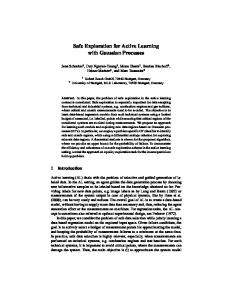
Figure 1. Plots of the log marginal likelihood over 4 runs of GPCMA using 4 different datasets.

answers. Hence, if for example, all 7 annotators assign the same label to some data point, the variance associated with that data point will be lower than when the 7 annotators provide contradicting labels. Figure 1 shows plots of the (negative) log marginal likelihood over 4 runs of GPC-MA using 4 different datasets, where it becomes clear the effect of the re-estimation of the annotator’s parameters α and β, which is evidenced by the periodic “steps” in the log marginal likelihood. 4.2. Real annotators The proposed approach was also evaluated on real multiple-annotator settings by applying it to the datasets used in (Rodrigues et al., 2013a) and made available online by the authors. These consist on a sentiment polarity and a music genre classification dataset. The former contains 5000 sentences from movie reviews extracted from the website RottenTomatoes.com and whose sentiment was classified as positive or negative, while the latter contains 700 samples of songs with 30 seconds of length and divided among 10 different music genres: classical, country, disco, hiphop, jazz, rock, blues, reggae, pop and metal. Both datasets were published on Amazon Mechanical Turk for annotation, and the authors collected a total 27747 and 2946 labels for training, corresponding to 203 and 44 distinct annotators, respectively. For both tasks, separate test sets are provided. The test set for the sentiment task consists of 5429 sentences while the test set for the music genre task contains 300 samples. For further details on these datasets, the interested readers are redirected to the original paper (Rodrigues et al., 2013a). Tables 3 and 4 show the results obtained for the different approaches in the sentiment and music datasets respectively. Since the music dataset corresponds to a multi-class

Trainset AUC F1 1.000 1.000 0.926 0.700 0.812 0.653 0.943 0.702

Testset AUC F1 0.852 0.683 0.695 0.423 0.661 0.411 0.882 0.601

Table 4. Results obtained for the music genre dataset.

problem, we proceeded by transforming it into 10 different binary classification tasks. Hence, each task corresponds to identifying songs of each genre. Unlike the previous experiments, with the music genre dataset a squared exponential covariance function with Automatic Relevance Determination (ARD) was used, and the hyper-parameters were optimized by maximizing the marginal likelihood. Due to the computational cost of the GPC-CONC approach and the size of the sentiment dataset, we were unable to test this method on this dataset. Nevertheless, the obtained results show the overall advantage of GPC-MA over the baseline methods. 4.3. Active learning The active learning heuristics proposed were tested on the music genre dataset from Section 4.2. For each genre, we randomly initialize the algorithm with 200 instances and then perform active learning for another 300 instances. In order to make active learning more efficient, in each iteration we rank the unlabeled instances according to eq. 11 and select the top 10 instances to label. For each of these instances we query the best annotator according to the heuristic we proposed for selecting annotators (eq. 12). Since each instance in the dataset is labeled by an average of 4.21 annotators, picking a single annotator per instance corresponds to savings in annotation cost of more than 76%. Each experiment is repeated 30 times with different random initializations. Figure 2 shows how the average testset AUC for the different music genres evolves as more labels are queried. We compare the proposed active learning methodology with a random baseline. In order to make clear the individual contributions of each of the heuristics proposed, we also show the results of using only the heuristic in eq. 11 for selecting an instance to label and selecting the annotators at random. As the figure evidences, there is a clear advantage in using both active learning heuristics together, which can provide an improvement in AUC of more than 10% after the 300 queries.

Gaussian Process Classification and Active Learning with Multiple Annotators blues

classical

the baseline methods. Furthermore, two simple and yet effective active learning heuristics were proposed, which can provide an even further boost in classification performance, while reducing the number of annotations required, and consequently the annotation cost.

0.92 0.75 AUC

0.9 0.74 0.88 0.73 0.86

0.72 100

200

300

100

country 0.8

AUC

300

200

300

0.76

0.78

0.74

0.76

0.72

0.74

0.7

0.72 0.7

200 disco

0.68 100

200

300

100

hiphop

The proposed approach makes the assumption that the labels provided by the different annotators do not depend on the instance their labeling, i.e. p(y r |z, x) = p(y r |z). Future work will try to relax this assumption by considering dependencies on x, and by modeling p(y r |z, x) with a Gaussian process. Regarding active learning, future work will also explore ways of jointly selecting the instance to label and the best annotator to label it.

jazz

Acknowledgments

0.85

0.84 AUC

0.84 0.82

0.83 0.82

0.8

0.81 0.78 100

200

300

100

metal

300

pop 0.75

0.66 AUC

200

References

0.74

0.64

0.73 0.72

0.62

0.71

0.6

0.7 100

The Fundaça˜ o para a Ciência e Tecnologia (FCT) is gratefully acknowledged for founding this work with the grants SFRH/BD/78396/2011 and PTDC/EIA-EIA/115014/2009 (CROWDS).

200

300

100

reggae

200

300

rock

0.84

Bachrach, Y., Graepel, T., Minka, T., and Guiver, J. How to grade a test without knowing the answers - a Bayesian graphical model for adaptive Crowdsourcing and aptitude testing. In Proc. of the 29th Int. Conf. on Machine Learning, 2012.

0.64 0.62

AUC

0.82

Barber, D. Bayesian reasoning and machine learning. Cambridge University Press, 2012.

0.6 0.58

0.8

0.56 0.54

0.78 100 200 num. queries

300 random pick instance pick both

100 200 num. queries

300

Figure 2. Active learning results on music genre dataset.

5. Conclusion and future work This paper presented the generalization of the Gaussian process classifier (a special case when R = 1, α = 1 and β = 1), a non-linear non-parametric Bayesian classifier, to multiple-annotator settings. By treating the unobserved true labels as latent variables, this model is able to estimate the different levels of expertise of the multiple annotators, thereby being able to compensate for their biases and thus obtaining better estimates of the ground truth labels. We empirically show, using both simulated annotators and real multiple-annotator data collected from Amazon Mechanical Turk, that while this model only incurs in a small increase in the computational cost of approximate Bayesian inference with EP, it is able to significantly outperform all

Chen, X., Lin, Q., and Zhou, D. Optimistic knowledge gradient policy for optimal budget allocation in crowdsourcing. In Proc. of the 30th Int. Conf. on Machine Learning, pp. 64–72, 2013. Dawid, A. P. and Skene, A. M. Maximum likelihood estimation of observer error-rates using the EM algorithm. Journal of the Royal Statistical Society. Series C, 28(1): 20–28, 1979. Groot, P., Birlutiu, A., and Heskes, T. Learning from multiple annotators with Gaussian processes. In Proc. of the 21st Int. Conf. on Artificial Neural Networks, volume 6792, pp. 159–164, 2011. Howe, J. Crowdsourcing: why the power of the Crowd is driving the future of business. Crown Publishing Group, New York, NY, USA, 1 edition, 2008. Kapoor, A., Grauman, K., Urtasun, R., and Darrell, T. Active learning with Gaussian processes for object categorization. In Int. Conf. on Computer Vision (ICCV), pp. 1–8, 2007.


Lawrence, N. D., Seeger, M., and Herbrich, R. Fast sparse Gaussian process methods: the informative vector machine. In Advances in Neural Information Processing Systems 15, pp. 609–616. MIT Press, 2003. Liu, C. and Wang, Y. TrueLabel + Confusions: a spectrum of probabilistic models in analyzing multiple ratings. In Proc. of the 29th Int. Conf. on Machine Learning, 2012. Minka, T. Expectation Propagation for approximate Bayesian inference. In Proc. of the 17th Conference in Uncertainty in Artificial Intelligence, pp. 362–369, 2001. Rasmussen, C. E. and Williams, C. Gaussian processes for machine learning (Adaptive computation and machine learning). The MIT Press, 2005. Raykar, V., Yu, S., Zhao, L., Valadez, G., Florin, C., Bogoni, L., and Moy, L. Learning from Crowds. Journal of Machine Learning Research, pp. 1297–1322, 2010. Rodrigues, F., Pereira, F., and Ribeiro, B. Learning from multiple annotators: distinguishing good from random labelers. Pattern Recognition Letters, pp. 1428–1436, 2013a. Rodrigues, F., Pereira, F., and Ribeiro, B. Sequence labeling with multiple annotators. Machine Learning, pp. 1–17, 2013b. Snow, R., O’Connor, B., Jurafsky, D., and Ng, A. Cheap and fast - but is it good?: Evaluating non-expert annotations for natural language tasks. In Proc. of the Conf. on Empirical Methods in Natural Language Processing, pp. 254–263, 2008. Welinder, P., Branson, S., Belongie, S., and Perona, P. The multidimensional wisdom of crowds. In Advances in Neural Information Processing Systems 23, pp. 2424– 2432, 2010. Wu, O., Hu, W., and Gao, J. Learning to rank under multiple annotators. In Proc. of the 22nd Int. Joint Conf. on Artificial Intelligence, pp. 1571–1576, 2011. Yan, Y., Rosales, R., Fung, G., Schmidt, M., Valadez, G., Bogoni, L., Moy, L., and Dy, J. Modeling annotator expertise: Learning when everybody knows a bit of something. Journal of Machine Learning Research, 9:932– 939, 2010. Yan, Y., Rosales, R., Fung, G., and Dy, J. Active learning from Crowds. In Proc. of the 28th Int. Conf. on Machine Learning, pp. 1161–1168, 2011.