Gene Classification Artificial Neural System
Cathy H. Wu
Corresponding Author: Cathy H. Wu, Ph.D. Associate Professor of Biomathematics Mailing Address: Department of Epidemiology/Biomathematics The University of Texas Health Center at Tyler P. O. Box 2003 Tyler, TX 75710 Federal Express Address: Department of Epidemiology/Biomathematics The University of Texas Health Center at Tyler US HWY 271 at State HWY 155 Tyler, TX 75708 Phone: Fax:
(903) 877-7962 (903) 877-5914
E-Mail Address:
[email protected] World Wide Web URL: http://diana.uthct.edu/~wu (Home page linked to GenCANS) Running Title: Gene Classification Artificial Neural System Invited Chapter For: Computer Methods for Macromolecular Sequence Analysis (A volum of Methods in Enzymology) Edited by Russell F. Doolittle, Academic Press.
Gene classification Artificial Neural System By Cathy H. Wu
Introduction As technology improves and molecular sequencing data accumulates exponentially, continued progress in the Human Genome Project will depend increasingly on the development of advanced computational tools for rapid annotation and easy organization of genomic sequences. Currently, a database search for sequence similarities represents the most direct computational approach to decipher the codes connecting molecular sequences with protein structure and function. 1 A sequence classification method can be used as an alternative approach to the database search/organization problem with several advantages: (1) speed, because the search time grows with the number of sequence classes (families), instead of the number of sequence entries; (2) sensitivity, because the search is based on information of a homologous family, instead of any sequence alone; and (3) automated family assignment.2 There are many different types of classification learning systems, broadly categorized into parametric and nonparametric models.3 The nonparametric classifiers do not require a priori recognition of certain specific patterns and make few assumptions in characterizing the samples. Some examples include the nearest-neighbor families of statistical methods and neural network algorithms, such as back-propagation 4 and counter-propagation. 5 As a technique for computational analysis, neural network technology has been applied to many studies involving sequence data analysis,6 including protein structure prediction, 7 identification of protein-coding sequences,8,9 and prediction of promoter sequences. 10 Several sequence classification methods have been devised, including our back-propagation neural network method,11 a multivariate statistical technique,12 a binary similarity comparison followed by an unsupervised learning procedure,13 and Kohonen's self-organized feature map.14 All of these classification methods are very fast, thus, applicable to the large sequence databases. The major difference between our and other approaches is that the back-propagation neural network is based on "supervised" learning, whereas the others are "unsupervised". The supervised learning can be performed using training sets compiled from any existing second generation database (i.e., database organized according to family relationship) and used to classify new sequences into the database according to the predefined organization scheme of the database. The unsupervised system, on the other hand, defines its own family clusters and can be used to generate new second generation databases. This chapter describes the gene classification artificial neural system (GenCANS), the neural network system we have developed for genetic sequence classification, and discusses future system enhancement and applications. GenCANS is a combined version of ProCANS (protein classification artificial neural system)15 and NACANS (nucleic acid classification artificial neural system).11 ProCANS was designed for the automatic classification of protein sequences according to the PIR (Protein Identification Resources) superfamilies15 and was extended into a full-scale
system for classification of more than 3300 protein superfamilies.16 In parallel, NACANS was developed for nucleic acid sequence classification by employing similar design principles. A network was implemented for classification of ribosomal RNAs (rRNAs) according to RDP (Ribosomal Database project) phylogenetic classes.17
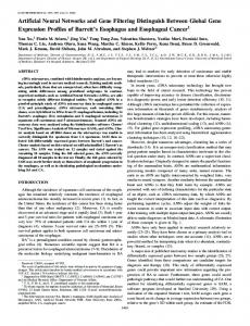
GenCANS Algorithm The neural network system was designed to classify new (unknown) sequences into predefined (known) classes. It involves two steps, sequence encoding and neural network classification, to map molecular sequences (input) into gene families (output) (Fig. 1). Sequence Encoding Schema The sequence encoding schema, used in the preprocessor, converts molecular sequences (character strings) into input vectors (numbers) of the neural network classifier (Fig. 1). An ideal encoding scheme should satisfy the basic coding assumption so that similar sequences are represented by 'close' vectors. There are two different approaches for the sequence encoding. One can either use the sequence data directly, as in most neural network applications of molecular sequence analysis, or use the sequence data indirectly, as in Uberbacher and Mural. 8 Where sequence data was encoded directly, most studies7,9 used an indicator vector to represent each molecular residue in the sequence string. That is to use a vector of 20 input units (among which 19 have a value of zero, and one has a value of one) to represent an amino acid, and a vector of four units (three are zeroes and one is one) for a nucleotide. This representation, however, is not suitable for sequence classification where long and varied-length sequences are to be compared. N-gram Method. We have been using an n-gram hashing method2,15 that extracts and counts the occurrences of patterns (terms) of n consecutive residues (i.e., a sliding window of size n) from a sequence string. Unlike the FastA method18, which also uses n-grams (k-tuples), our search method uses the counts, not positions, of the n-gram terms along the sequence. Therefore, our method is length-invariant, provides certain insertion/deletion invariance, and does not require the laborious sequence alignments of many other database search methods. The counts of the n-gram terms from each encoding method are scaled to fall between 0 and 1 and used as input vectors for the neural network, with each unit of the vector representing an n-gram term. The size of the input vector for each n-gram extraction is mn, where m is the size of the alphabet. The original sequence string can be represented by different alphabet sets in the encoding. The alphabet sets used for protein sequences include the 20-letter amino acids and the six-letter exchange groups derived from the PAM (accepted point mutation) matrix. The alphabet for nucleic acid sequences is the four letter AT(U)GC. The major drawback of the n-gram method is that the size of the input vector tends to be large. This indicates that the size of the weight matrix (i.e., the number of neural interconnections) would also be large because the weight matrix size equals to w, where w = input size x hidden size + hidden size x output size. This prohibits the use of larger n-gram sizes, e.g., the trigrams of amino
acids would require 20 3 or 8000 input units. Furthermore, accepted statistical techniques and current trends in neural networks favor minimal architecture (with fewer neurons and interconnections) to avoid data overfitting and provide better generalization capability. 19 SVD (Singular Value Decomposition) method. The SVD method16 is used to reduce the size (i.e., the number of dimensions) of the n-gram vectors and to extract semantics from the n-gram patterns. The method was adopted from the Latent Semantic Indexing analysis used in the field of information retrieval and information filtering. The approach is to take advantage of implicit high order structure in the association of terms with documents in order to improve the detection of relevant documents which may or may not contain actual query terms. In SVD, the n-gram term matrix (i.e., term-by-sequence matrix) is decomposed into a set of k orthogonal factors from which the original matrix can be approximated by linear combination. The reduced model can be shown by: X ~ Y = TSP'
(1)
where X is the original term matrix, Y is the approximation of X with rank k, T and P are the matrices of left and right singular (s) vectors corresponding to the k-largest s-values, and S is the diagonal matrix of the k-largest s-values. Note that if X is used to represent the original term matrix for training sequences, then P becomes the reduced matrix for the training sequences. The representation of unknown sequences is computed by "folding" them into the k-dimensional factor space of the training sequences. The folding technique, which amounts to placing sequences at the centroid of their corresponding term points, can be expressed by: Pu = Xu'TS-1
(2)
where Pu and Xu are the reduced and original term matrices of unknown sequences, T is the matrix of left s-vectors computed from Eq. 1 during training phase, and S-1 is the inverse of S, which reflects scaling by reciprocals of corresponding s-values. It has been shown that, as with the n gram sequence encoding method, the SVD method also satisfies the basic coding assumption.16 Neural Network Paradigm Back-Propagation (BP) Networks. The BP neural networks in GenCANS are three-layered, feed forward networks 15 (Fig. 1). A feedforward calculation (change of state function) is used to determine the output of each neuron as in: Oi = f (∑OjWij) = f (neti) = 1 / (1 + e(-neti+θ))
(3)
where O j represents the output from the neuron j in the preceding layer, W ij represents the connection weight between neurons i and j, neti is the net input to each neuron, is a bias term, and f is a nonlinear activation (squashing) function. The back-propagation learning applies the generalized delta rule to recursively calculate the error signals and adjust the weights (Eqs. (4) -
(6)). The error signal at the output layer is given by: δi = f'(neti) (Ti - Oi)
(4)
where Ti is the target value, and f'(neti) is the first derivative of the activation function. The error signal at the hidden layer is given by: δj = f'(netj)∑ Wijiδi i
(5)
The error signals are then used to modify the weights by: ∆Wij(t+1) = ηOjδι + α∆Wij(t)
(6)
where η is the learning rate and α is the momentum term. In the BP network, the size of the input layer (i.e., number of input units) is dictated by the sequence encoding schema chosen. The size is mn with n-gram encoding; and the size is the reduced dimension (k), if the n-gram vector is compressed by SVD. The output layer size is determined by the number of classes represented in the network, with each output unit representing one class. The hidden size is determined heuristically, usually a number between input and output sizes. In GenCANS, the networks are trained using weight matrices initialized with random weights ranging from -0.3 to 0.3. Other network parameters include a learning factor of 0.3, a momentum term of 0.2, and a constant bias term of -1.0. Back-Propagation with Pattern Selection Strategy (BPS). One major problem frequently encountered when using BP neural networks is the long training time. In BP, all patterns in the training set are usually presented equally to the neural network (i.e., uniform presentation). To speed up the BP training, a pedagogical pattern selection strategy17 is used to favor the selection of patterns producing high error values to the disadvantage of the patterns already mastered by the network. In GenCANS, a modified EDR (error-dependent repetition) method is used, in which training proceeded as described20 for the first 400 iterations, followed by another 100 iterations using all training patterns with uniform presentation. Counter-Propagation (CP) Networks. A modified CP algorithm21 with supervised LVQ (learning vector quantizer) and dynamic node allocation is another learning paradigm used. The forward-only CP network has three layers (an input layer, a Kohonen layer and a Grossberg outstar conditioning layer). As in BP network, the sizes of the input and output (Grossberg) layers are the size of the input vector and the number of output classes, respectively. The size of the hidden (Kohonen) layer is configured dynamically during the course of training. In our modified algorithm, n (n = number of classes) Kohonen nodes are allocated initially, with their weights initialized to be the average input vector of each class. During the training phase, nodes are added dynamically when any given training pattern fails to be assigned to the Kohonen units that represents its class. The weight vector of the newly added node is then assigned with the input
vector of the untrainable pattern. The network training involves two steps, to select a winner and to update the winner's weight vector. The winner, selected based on a spherical arc distance measure (Eq. (7)), is the Kohonen unit whose weight vector is closest to the input vector (i.e., with the highest weighted sum or smallest angle). The spherical arc distance between the normalized, unit-length input vector (X) and weight vector (Wj) is computed by: Sj = ∑xiwij = X . Wj = cos θj
(7)
where xi is the activation level of input unit i, wij is the weight from input unit i to Kohonen unit j, Sj is the weighted sum for Kohonen unit j, and j is the angle between X and Wj. The sum equals the dot product of the input and weight vectors. A supervised learning that selects two winners with punishment mechanism is used for weight update: if the first winner is correct, it is updated with positive weight (Eq. 8), otherwise, the winner is punished with negative weight (Eq. 9) and the second winner is chosen; if the second winner is correct, it is updated with positive weight, if incorrect, a new unit is allocated. The weight adjustments for correct and incorrect winners are given by the Kohonen learning law: wic (t+1) = wic (t) + α (xi - wic)
(8)
wic (t+1) = wic (t) - α (xi - wic)
(9)
where α is the learning rate (0 < α < 1.0); and w(t) and w(t+1) are the weights from previous iteration and for current iteration, respectively. The Kohonen learning rate for weight adjustment is chosen as 0.2.
GenCANS Implementation GenCANS Systems Presently, we have implemented two GenCANS systems, GenCANS_PIR for full-scale classification of protein sequences into PIR superfamilies, and GenCANS_RDP for classification of rRNAs according to RDP phylogenetic classes. GenCANS_PIR. The system was trained with the PIR database22 (Release 44.0, March 31, 1995) using a modular network architecture2 that involves multiple independent neural networks to partition different protein functional groups. The database has three sections, PIR1 for annotated and classified entries, PIR2 for annotated but not classified or tentatively classified sequences, and PIR3 for unverified entries. The classification in PIR is based on the superfamily concept. A superfamily is a group of proteins that share sequence similarity due to common ancestry, and sequences within a superfamily have a less than 10 -6 probability of similarity by chance. The training set for the GenCANS_PIR consisted of all PIR1 entries in 3,462 superfamilies, partitioned
into 15 modules (Table I). During the training phase, each network module was trained separately using the sequences of known superfamilies; during the prediction phase, unknown sequences were classified on all modules with classification results combined. All PIR2 entries, which had tentative superfamily assignment and were at least 30 amino acids long, were used in the prediction set for system evaluation. GenCANS_RDP. The system was trained with the RDP database23 (Release 5.0, May 17, 1995). There are three collections of rRNA sequences, the SSU_Prok (prokaryotic small subunit), SSU_Euk (eukaryotic small subunit), and LSU (large subunit). A total of 220 SSU (177 Prok + 43 Euk) classes, containing 3,285 (2,849 Prok + 436 Euk) sequence entries, were derived directly from the SSU_Prok.phylo and SSU_Euk.phylo phylogenetic listing files in the RDP database. Similarly, 15 LSU classes containing 72 sequences were derived from the LSU.phylo file. In the SSU classification scheme, no one class at the non-leaf level had more than 50 sequence entries (i.e., for any class that had more than 50 entries at one given level, it was further subdivided into classes at its sublevel, unless it reached the leaf level). The classes may be at different levels in the tree. 17 The finest level of classification would be to use one neural network class to represent every single leaf node on the phylogenetic tree. This would yield a total of 287 classes for SSU sequences. The LSU sequences, on the other hand, were classified at the leaf level. Table II gives a partial list of the phylogenetic classes of SSU and LSU sequences. To test the system performance, a three-fold cross-validation method21 was used to partition the data set. The data was randomly divided into three approximately equal sized sets; and in each trial one set was used for prediction and the union of the others for training. Program Structure As shown in the GenCANS structure chart (Fig. 2), the system software has three major components: a preprocessor to create from input sequence files the training and prediction patterns, a neural network program to classify input patterns, and a postprocessor to summarize classification results. The preprocessor has subprograms for n-gram encoding (ngram), SVD computation (svd), and combining different sequence encoding algorithms (comb). The neural network program has subprograms for standard back-propagation (bp), back-propagation with pattern selection strategy (bps), and counter-propagation (cp). The postprocessor ranks all classification scores and provides identifications for top-ranking classes. All programs were coded in C language and implemented on the Cray Y-MP8/864 supercomputer of the University of Texas System. The programs have also been ported to several other UNIX computer platforms, including a DEC alpha workstation, and a Silicon Graphics workstation. GenCANS (version 2.0, 1995)24 is a software package that provides various functions needed to use the classification systems in an integrated environment. Through either the command line or a menu interface, the user can work on either protein or DNA/RNA sequences, either training or prediction mode, either single-module or multiple-module neural networks, and either a single encoding algorithm or several combined algorithms. There are also many utility functions for tracking system performance, maintaining a system log, and converting file formats. Program Availability
GenCANS is available on the Internet via World Wide Web (WWW) (http://diana.uthct.edu) or by anonymous FTP from diana.uthct.edu. A distribution version of the GenCANS_RDP can be found in the compressed "tar" file (gencans_rdp.tar.Z). The version consists of all source codes needed for network prediction, the trained network weight files, sample input and output files, and README. The source programs were written in ANSI C, and should be able to compile and run on any UNIX machines with a C/C++ compiler. During installation, a total of about 200 MBytes disk space is needed, after which some intermediate files would be removed (by the makefile), and the total disk space needed to store all files is less than 60 MBytes. The present distribution version can be used for speedy on-line rRNA sequence classification with the weight files obtained from off-line training. A distribution version for GenCANS_PIR will be prepared and made available from the same site. Future releases may contain programs for network training and prediction to provide both on-line training and classification capabilities. Furthermore, our WWW server allows users to perform direct PIR or RDP sequence classifications by entering a sequence using a WWW client program, such as Mosaic or Netscape. The query will be configured to automatically generate and submit an appropriate query to be searched on our WWW server. The search results are then returned to the client as a HyperText Markup Language (HTML) document (Table III).
GenCANS Evaluation Evaluation Mechanism The system performance is measured by its speed (CPU time) and predictive accuracy. The predictive accuracy is expressed with three terms: the total number of correct patterns (true positives), the total number of incorrect patterns (false positives), and the total number of unidentified patterns (false negatives). A sequence entry is considered to be accurately classified if one of its top-ranking classes matches the target class with a classification score above the threshold (i.e., the cut-off value). The classification score ranges from 1.0 for perfect match to 0.0 for no match. In this study, results for correct patterns are reported using two measures, the first fit (the class with the highest score matches the target) and the first n-fits (one of the classes with the n highest scores matches the target). Performance of GenCANS_PIR System The result of the GenCANS_PIR system is shown in Table IV. The training of 12,572 sequences on the fifteen network modules took a total of 2.2 Cray CPU hours, which averaged to 0.63 second per sequence. (Without the pedagogical pattern selection strategy, the training would be about five times longer). Among all training patterns, 99.68% were trained into appropriate classes after 500 iterations. Majority of the remaining "untrainable patterns" belonged to single membered or double-membered superfamilies, as one would expect. The prediction of an unknown sequence on all fifteen networks took an average of 0.62 CPU second on a DEC alpha
workstation. (The equivalent BLAST25 search took 18 seconds, or approximately 30 times longer on the same workstation). At a threshold of 0.1, 80.55% patterns were correctly classified as first-fit. If we consider the top ten fits (among a total of 3,462 possible classes) as correct classification, then the predictive accuracy of the full-scale system was 87.72%. To make the "mega-classification" helpful, one can use a much higher threshold to reduce the number of false positives. At a threshold of 0.9, although only 51.54% patterns were correctly classified, the incorrectly classified entries were reduced to 0.23%. The remaining entries were not classified at this threshold. Again, most of the entries failed to be classified (correctly predicted) by the neural nets were those in single-membered or double-membered superfamilies, which account for half and one-sixth of all PIR superfamilies, respectively. When only the fifty largest superfamilies were used, more then 98% of the sequences were correctly classified as the first-fit at the threshold of 0.1; and close to 90% of the entries were classified with a classification score of more than 0.9, with no false positives.16 It should also be noted that not all entries "misclassified" by the neural network are truly misclassified. Indeed, a few erroneous superfamily placements have been identified (personal communication with Dr. Barker of NBRF-PIR) by the neural network using the high threshold of 0.9. Performance of GenCANS_RDP System The training of the entire RDP system (for 3,285 SSU and 72 LSU sequences on both BPS and CP networks) took about 1.4 Cray CPU hours. The training time for individual networks is shown in Table IV. The prediction of an unknown sequence took approximately 0.3 DEC CPU second (Table IV), about an order of magnitude faster than other search methods, including BLAST and Similarity Rank.17 The predictive accuracy measured using three-fold cross validation indicates that the BP and CP networks had similar accuracy and their combination yielded best results, close to 99% for SSU and 100% for LSU prediction (Table IV). The time required to obtain the combined results (i.e., Avg(BPS,CP)) is about the same as that for individual BPS or CP network, because the actual network prediction took very little time. As observed before,17 for query sequences whose correct class appeared as second or third-fit, their first and second-fit classes were also closely located on the phylogenetic tree.
Discussion This chapter describes two neural network sequence classification systems, GenCANS_PIR for PIR superfamily placement of protein sequences, and GenCANS_RDP for RDP phylogenetic classification of rRNA sequences. The major applications of the classification neural networks are rapid sequence annotation and automated family assignment. Currently, the classification speed of GenCANS is about an order of magnitude faster then other methods. The rate gap will continue to widen with the accelerated growth of molecular sequence databases. Unlike most other sequence comparison or database search methods in which search time is directly proportional to the number of sequence entries in the database, the neural network
classification time is expected to remain low even if there is a 100 to 1000 fold increase of sequence entries. This is because that the total network classification time is dominated by the preprocessing time (i.e. more than 95% of the total time), and that the n-gram and SVD computation time required for preprocessing query sequences is determined by the size of the n gram vectors, but independent of the number of training sequences. The full-scale PIR classification system can be used as a filter program for other database search methods to minimize the time required to find relatively close relationships. Similarly, classification of unknown rRNA sequences into predefined classes on a phylogenetic tree, without sequence alignment, is a rapid means of sequence annotation. Ribosomal RNA sequences are now the method of choice for surveying the biosphere. The rRNA classification system can be used to screen large collections of short rRNA sequences, such as those produced by environmental characterizations, in order to identify those worthy of more complete sequence determination. The neural classification system can also be used to automate family assignment. The tool is generally applicable to any molecular databases that are developed according to family relationships because the neural networks employ supervised learning algorithms. An automated classification tool is especially important for the organization of database according to family relationships and for handling the influx of new data in a timely manner. Among all entries in the PIR database, only a small fraction are classified and placed in superfamilies. The neural network system is currently being used by the PIR database for superfamily identification of unclassified sequences. Likewise, the size of the RDP database continues to grow, with a doubling rate over the last five years, and the phylogenetic tree placement gradually lags. The neural network tool can be used by the RDP database to automate family assignment and help build the phylogenetic tree. There are two major directions for future research, to improve the classification accuracy, and to extend the current designs for developing a gene identification system. The current n-gram sequence encoding method, although effective in preserving sequence similarity, encodes "global" information only. The capability to encode "local" information conserved in the motif regions, however, is essential, since information content from the entire sequence string is not equal. We have recently developed a new database search algorithm, termed MOTIFIND (Motif Identification Neural Design),26 for rapid and sensitive protein family identification. The method employs an n gram term weighting algorithm for extracting motif patterns and integrated neural networks for combining global and local information, and has shown a significant improvement in predictive accuracy. The design of the neural system can be easily extended to classify other nucleic acid sequences. Preliminary studies have been conducted to classify DNA sequences (containing both protein-encoding regions and intervening sequences) directly into protein superfamilies with satisfactory results. It is, therefore, possible to develop a gene identification system that can classify indiscriminately sequenced DNA fragments.
Acknowledgments This research is supported in part by the grant number R29 LM05524 from the National Library of Medicine, and by the University Research and Development Grant Program of the Cray Research, Inc.
REFERENCES 1
2 3
4
5 6 7 8 9 10 11
12 13
14 15
16 17 18 19
20 21 22
23
24
25
26
R. F. Doolittle, in "Molecular Evolution: Computer Analysis of Proteins and Nucleic Acid Sequences, Methods in Enzymology, Vol. 183" (R. F. Doolittle, ed.), p. 99, Academic Press, New York, 1990. C. H. Wu, Comp. Chem., 17, 219 (1993). S. M. Weiss and C. A. Kulikowski, "Computer systems that learn: Classification and prediction methods from statistics, neural nets, machine learning, and expert systems," Morgan Kaufmann Publishers, Inc., San Mateo, CA, 1991. D. E. Rumelhart and J. L. McClelland, (eds), "Parallel Distributed Processing: Explorations in the Microstructure of Cognition. Volume 1: Foundations," MIT Press, 1986. R. Hecht-Nielsen, Applied Optics, 26, 4979 (1987). J. D. Hirst and M. J. E. Sternberg, Biochemistry, 31, 7211 (1992). N. Qian and T. J. Sejnowski, J. Mol. Biol., 202, 865 (1988). E. C. Uberbacher and R. J. Mural, Proc. Natl. Acad. Sci., U.S.A., 88, 11261 (1991). R. Farber, A. Lapedes, and K. Sirotkin, J. Mol. Biol., 226, 471 (1992). M. C. O'Neill, Nuc. Acids Res., 20, 3471 (1992). C. H. Wu, in "The Protein Folding Problem and Tertiary Structure Prediction," (Kenneth Merz and Scott LeGrand, eds), p. 279, Birkhauser Boston, Inc., 1994. M. van Heel, J. Mol. Biol., 220, 877 (1991). N. Harris, L. Hunter, and D. States, in "Proceedings of 10th National Conference on Artificial Intelligence," p. 837, AAAI Press, 1992. E.A. Ferran, B. Pflugfelder, and P. Ferrara, Protein Science, 3, 507 (1994). C. H. Wu, G. Whitson, J. McLarty, A. Ermongkonchai, and T. Chang, Protein Science, 1 , 667 (1992). C. H. Wu, M. Berry, S. Shivakumar, and J. McLarty, Machine Learning, (in press). C. H. Wu and S. Shivakumar, Nuc. Acids Res., 22, 4291 (1994). W. R. Pearson and D. J. Lipman, Proc. Natl. Acad. Sci., U.S.A., 85, 2444 (1988). Y. Le Cun, J. Denker, and S. Solla, in "Advances in Neural Information Processing Systems 2," p. 598, San Mateo, CA: Morgan Kaufman, 1990. C. Cachin, Neural Networks, 7, 175 (1994). C. H. Wu, H. L. Chen, and S. C. Chen, Applied Intelligence, (in press). D. G. George, W. C. Barker, H. -W. Mewes, F. Pfeiffer, and A. Tsugita, Nuc. Acids Res., 22, 3569 (1994). B. L. Maidak, N. Larsen, M. J. McCaughey, R. Overbeek, G. J. Olsen, K. Fogel, J. Blandy, and C. R. Woese, Nuc. Acids Res., 22, 3485 (1994). H. L. Chen and C. H. Wu, "GenCANS User's Guide," University of Texas Health Center at Tyler, 1995 (available on our WWW server). S. F. Altschul, W. Gish, W. Miller, E. W. Myers, and D. J. Lipman, J. Mol. Biol., 215, 403 (1990). C. H. Wu, H. L. Chen, and J. W. McLarty, (Submitted).
FIGURE CAPTIONS
Fig. 1. The gene classification artificial neural system (GenCANS) for molecular sequence classification. The sequence strings are first converted by an n-gram sequence encoding method into input vectors of real numbers. Long n-gram input vectors can be compressed by a SVD method to reduce vector size (dimension). The neural network then maps the sequence vectors into predefined classes according to sequence information embedded in the neural interconnections after network training. The neural networks used are three-layered, feed-forward networks that employ the back-propagation or counter-propagation learning algorithm. Fig. 2. GenCANS structure chart.
Table I. Neural network modules of the GenCANS_PIR for partitioning superfamilies. ______________________________________________________________________________ Network Protein Superfamilies NumberofEntriesa Module Functional Groups Begin-End Total PIR1 PIR2 ______________________________________________________________________________ EO Electron Transfer Proteins , Oxidoreductases 1- 209 209 1227 1880 TR Transferases 210- 478 269 926 828 HY Hydrolases 479- 739 261 972 1161 LI Lyases, Isomerases, Ligases 740- 934 195 763 446 PG Protease Inhibitors, Growth Factors, Hormones, Toxins 935-1185 251 1154 1493 IH Immunoglobulin-Related, Heme Carrier, Chromosomal, Ribosomal proteins 1186-1378 193 1794 2022 FL Fibrous, Contractile system, LipidAssociated Proteins, Miscellaneous 1379-1632 254 1151 1810 PM Plant, Membrane, Organelle Proteins 1633-1838 206 533 862 BP Bacterial Proteins 1839-2059 221 432 599 AD Bacteriophage, Plasmid, Yeast, Animal DNA viral proteins 2060-2309 250 686 247 LH Large DNA Viral Proteins, Herpes Virus 2310-2481 172 463 70 LA Large Adnovirus, Vaccina Proteins 2482-2640 159 314 87 AR Animal RNA Viral Proteins 2641-2864 224 1378 557 PP Plant Viral, Phage Proteins 2865-3069 205 493 146 PH Phage T, Hypothetical proteins 3070-3462 393 286 494 Total 1-3462 3462 12,572 12,702 ______________________________________________________________________________ a The sequence entries in PIR1 (release 44.0) were used for training, and those in PIR2 for prediction.
Table II. A partial list of phylogenetic classes in the GenCANS_RDP. ______________________________________________________________________________ Class Number of Class ID Class Namea Number Sequences Numbera ______________________________________________________________________________ Small Subunit (SSU) 1 8 1.1.1 Archaea.Euryarchaeota.Methanococcales 2 19 1.1.2 Archaea.Euryarchaeota.Methanobacteriales .. 10 11
.. 39 6
...... 1.2 2.1
.............. Archaea.Crenarchaeota Bacteria.Thermophilic_Oxygen_Reducers
.. 135
.. 95
..... 2.15.1.12.2
.............. Bacteria.Gram_Positive_Phylum.High_G+C_Sub division.Mycobacteria
.. 177
.. 10
..... 2.15.5.16
178 179
17 2
3.1.1.1 3.1.1.2
.............. Ba cte ria . G ram _P o s it ive _P h ylu m. Bac ill us LactobacillusStreptococcus_Subdivision.Alicyclobacillus_Group Eukaryotes.Eumycota.Ascomycotina.Plectomycetes Eukaryotes . Eumycota. Ascomycotina.Loculoa scomycetes
.. 220
.. 10
..... 3.21
.............. Eukaryotes.Microsporidia
1.1 1.1.1
Archaea.Euryarchaeota Archaea.Euryarchaeota.Extreme_Halophiles .............. Bacteria.Flexibacter-Cytophaga-Bacteroides_Phylum
Large Subunit (LSU) 1 6 2 4 .. 5
.. 2
..... 2.1
.. 12
.. 2
..... 2.4.2
.............. Bacteria.Gram_Positive_Phylum.Clostridial_Subdi vision 13 11 3.1 Eukaryotes.Fungi_And_Protists 14 7 3.2 Eukaryotes.Plants 15 10 3.3 Eukaryotes.Animals ______________________________________________________________________________ a
The class ID number and name are directly taken from the SSU_Prok.phylo, SSU_Euk.phylo and LSU.phylo, the phylogenetic listing files in the RDP database, release 5.0.
Table III. Direct GenCANS_RDP search on World Wide Web server (http://diana.uthct.edu). ______________________________________________________________________________ (A) Input to GenCANS_RDP (entered via a WWW client) Sequence Name/identifier: rdp|Mc.jannasc Methanococcus jannaschii str. JAL-1. Sequencea: AUUCCGGUUGAUCCUGNNGGAGGCCACUGCUAUCGGGGUCCGACUAAGCCAUGC GAGUCAAGGGGCUCCCUUCGGGGAGCACCGGCGCACGGCUCAGUAACACGUGGC UAACCUA...............UUGCACACACCGCCCGUCACGCCACCCGAGUUGAGCCCAAG UGAGGCCCUGUCCGCAAGGGCAGGGUCGAACUUGGUAACAAGGAACCUGGAUCAC CUCC (B) Classification Result from GenCANS_RDP (returned as a HTML document) Sequence length: 1437 Class_ID Class_Score Class_Name 1.1.1.0.0 1.1.4.0.0 1.1.3.5.0
Archaea.Euryarchaeota.Methanococcales Archaea.Euryarchaeota.Thermococcales Archaea.Euryarchaeota.Methanomicrobacteria_and_Relatives.Archa eoglobales 1.1.5.0.0 0.45 Archaea.Euryarchaeota.Methanopyrales 1.1.2.0.0 0.45 Archaea.Euryarchaeota.Methanobacteriales ______________________________________________________________________________ a
0.98 0.48 0.47
Only a partial input sequence is shown.
Table IV. The training and prediction results of GenCANS. ______________________________________________________________________________ System Encodinga Networkb Networkc CPU Timed Predict Accuracy Method Algorithm Configuration Train Predict First-Fit N-Fits e ______________________________________________________________________________ PIR
a23e4_100
BPS
100 x 100 x (159-393)
0.63
0.62
80.55
87.72
RDP (SSU)
n8_100 n8_100
BPS 100 x 100 x 220 CP 100 x (339-393) x 220 Avg (BPS, CP)
1.50 0.75
0.28 0.28 0.29
96.07 94.91 96.26
97.64 98.53 98.74
RDP (LSU)
n8_40 n8_40
BPS 40 x 30 x 15 0.48 0.34 92.86 98.57 CP 40 x (17-18) x 15 0.40 0.32 94.29 98.57 Avg (BPS, CP) 0.35 92.86 100.00 ______________________________________________________________________________ a
b c
d
e
The "a23e4_100" method used the a23e4 n-gram method, followed by the SVD method to generate an input vector of 100 dimensions. The a23e4 n-gram method concatenated three separate n-gram vectors, namely, a2 (bigrams of amino acids), a3 (trigrams of amino acids), and e4 (tetragrams of exchange groups), and formed a vector of 9,696 units (i.e., 9696 = 202 + 203 + 64 ). The "n8_100/40" method used the n8 (octagrams of nucleic acids) n-gram method, followed by the SVD compression to reduce the input vector from 65,536 (i.e., 48) to 100/40 dimensions. BPS: Back-Propagation with pattern selection strategy; CP: Counter-Propagation; Avg (BPS, CP): classification results obtained from averaging the BPS and CP classification scores. The PIR system has fifteen neural network modules, each with a configuration of 100 x 100 x n, where n is the number of protein superfamilies in the module, ranging from 159 to 393 (Table I). The hidden size of the CP networks used in the RDP system was configured dynamically and varied for different data sets in ranges as indicated. The CPU time indicated is the average time per sequence and includes the total time for preprocessing, neural network learning/mapping, and postprocessing. The training time unit is Cray CPU second (on a Cray Y-MP), and the prediction time unit is DEC CPU second (on a DEC 3000 workstation). "N-Fits" is the top ten-fits (out of 3,462 superfamilies) for the PIR system, five-fits (out of 220 phylogenetic classes) for the RDP SSU system, and two-fits (out of 15 classes) for the RDP LSU system.
Unknown Sequence
Input Vector
Compressed Input Vector Neural Network
70
80
90
1000
60
800
50
SVD
40
DNA/RNA or Protein Class
0 1 0.9 0.8 0.7 0.6 0.5 0.4 0.3 0.2 0.1 0
200
10
20
400
30
600
N-gram Encoding
0
or
M A
S S T F Y I P F V N E . .
1 0.9 0.8 0.7 0.6 0.5 0.4 0.3 0.2 0.1 0
A TU G G C TU C C A TU C A A . .
100
DNA/RNA Protein
Input Layer
Hidden Output Layer Layer
TRAINING
PREDICTION
*.SEQ *.CNT
*.SEQ [*.CNT]
NGRAM *.KNW
*.INF
NGRAM *.KNW
*.INF
NGRAM *.UNK
NGRAM
*.INF
*.UNK *.INF
*.LAL
SVD *.KNW
*.UNK
COMB
*.KNW
PRE-PROCESSOR
SVD
COMB
*.INF
*.UNK
*.INF
*.WGT
BP / BPS / CP
BP / BPS / CP
*.OUT
*.INF
*.OUT
POST
POST
*.RPT
*.RPT
NEURAL NETWORK [*.LIS]
POST-PROCESSOR