reduced models by the proposed BSPRIM will still match the 2q moments and preserve the circuit structure properties like symme- try as SPRIM does.
General Block Structure-Preserving Reduced Order Modeling of Linear Dynamic Circuits ∗
Ning Mi† , Boyuan Yan† , Sheldon X.-D. Tan† , Jeffrey Fan† and Hao Yu‡
† Department
‡ Department
of Electrical Engineering, University of California, Riverside, CA 92521 of Electrical Engineering, University of California, Los Angeles, CA 90095
ABSTRACT
In this paper, we propose a generalized block structure-preserving reduced order interconnect macromodeling method (BSPRIM). Our approach extends structure-preserving model order reduction (MOR) method SPRIM [4] into more general block forms. We first show how SPRIM-like structure-preserving MOR method can be extended to deal with admittance RLC circuit matrices and show the 2q moments are still matched and symmetry is preserved. We then show that 2q moment matching can’t be achieved when the RLC circuits are driven by both current and voltage sources. The new approach also improves SPRIM by introducing the re-orthonormalization process on the partitioned projection matrix. Then we present our BSPRIM method to deal with more circuit partitions and show the resulting general block structure preserving MOR for linear dynamic circuits formulated in impedance and admittance forms. The reduced models by the proposed BSPRIM will still match the 2q moments and preserve the circuit structure properties like symmetry as SPRIM does. Experimental results demonstrate effectiveness of the proposed methods and it outperforms SPRIM in terms of accuracy with more partitions.
1.
INTRODUCTION
Compact modeling of passive RLC interconnect networks has been an research intensive area in the past decade due to increasing signal integrity effects and increasing design complexity in current system on a chip (SoC) design [6]. Reducing the many parasitic RLCK circuits by equivalent compact models in higher level simulation can significantly improve the simulation and verification process in nanometer VLSI designs. The most widely used method is based on subspace projection [8, 3, 9, 5, 7, 4]. Projection-based method was pioneered by Asymptotic Waveform Evaluation (AWE) algorithm [8] where explicit moment matching was used to compute dominant poles at low frequency. Pade via Lanczos (PVL) [3], Arnoldi Transformation method [9] improved the numerical stability of AWE, congruence transformation method [5] and PRIMA [7] can further produce passive models. However, reduced circuit matrices by PRIMA are larger than direct pole matching (having more poles than necessary) [1] and PRIMA does not preserve certain important circuit structure properties like reciprocity. Recently, a structure-preserving model reduction (SPRIM) is proposed in [4]. This approach partitions the state matrix in the MNA (modified nodal analysis) form into a natural 2 × 2 block matrices, i.e., conductance, capacitance, inductance, and adjacent matrices. Accordingly the projection matrix is partitioned. As a result, SPRIM matches the twice moments of the models by using the projection matrix given by PRIMA. The reduced models also
preserve the structure properties of the original models like symmetry (reciprocity). This idea has been extended to deal with the more partitions by block structure-preserving model order reduction (BSMOR) [10] to further exploit the regularity of the many parasitic networks. It was shown that by introducing more partitions, more poles are matched which leads to more accurate order reduced models [11]. However, BSMOR method simply introduce more partitions/blocksx, it does not truly preserve the circuit structures for general RLCK circuits for different input sources (voltages or currents). The reduced model does not match the 2q moments of the original models as SPRIM does. In this paper, we first show theoretically that structure-preserving model order reduction can be applied to RLCK admittance networks, which are driven by the voltage sources and requires partitioning of the original MNA circuit matrix into 2 × 2 block matrices. We further show that for a hybrid MNA circuit matrix where both current and voltage sources are present, 2q moment matching can’t be achieved. Then we proposed a general block structurepreserving reduced order modeling of interconnects (BSPRIM), which generalizes SPRIM method [4] by considering more partitions. We study the matrix partitioning for both impedance matrices and admittance matrices separately and show that the reduced models will still match the 2q moments of the original circuits and the circuit structures like symmetry, sparsity can be preserved. Experiments show that with more partitions, the reduced models become more accurate. The rest of the paper is organized as follows. We review the structurepreserving model order reduction in Section 2. Then we present the new method to extend SPRIM to deal with admittance matrix with voltage sources in Section 3. After this we present our BSPRIM method in Section 4 where how structure preserving can be extended to n × n cases for both impedance and admittance matrices and show the 2q moments still are matched and symmetric property is preserved. We present the experimental results in Section 5, and concludes the paper in Section 6. Proofs of some key theorems will be included in the appendix section.
2. BLOCK STRUCTURE PRESERVING MODEL REDUCTION In this section, we review the structure-preserving projection based MOR method SPRIM and the important results of SPRIM method.
2.1 Preliminary
Consider a modified nodal formulation (MNA) of the RLCK circuit equation in the frequency domain:
∗ This work is supported in part by NSF CAREER Award CCF0448534, UC Micro Program #04-088 and #05-111 via Cadence Design System Inc.
Proceedings of the 8th International Symposium on Quality Electronic Design (ISQED'07) 0-7695-2795-7/07 $20.00 © 2007
G x(s) + sC x(s) = B i p (s)
v p (s) = B T x(s)
(1)
where x(s) is the state variable vector, G and C (∈ RN×N ) are state matrices. B (∈ RN×n p ) is B = [BT1
0]T ,
(2)
a port incident matrix. We assume that we have only current sources indicated by i p (s) now. Eliminating x(s) in equation(1) gives v p (s) = H(s)i p (s) H(s) = B T (G + sC )−1 B ,
(3)
where H(s) is a multiple-input multiple-output (MIMO) impedance transfer function. PRIMA finds a projection matrix V (∈ RN×qn p ) such that its columns span the q-th block Krylov subspace K (A , R , q), i.e., spanV = K (A , R , q), (4) where A = (G + s0 C )−1 C , R = (G + s0 C )−1 B , and s0 is the expansion point that ensures G + s0 C is nonsingular. The resulting reduced transfer function is ¯ H(s) = B¯ T (G¯ + sC¯ )−1 B¯ , (5) where G¯ = V T G V,
C¯ = V T C V,
B¯ = V T B ,
(6) has the identical expanded first q-th moments of the original transfer function H(s). It is called as the Grimme’s projection theorem [2]. Note that G¯ , C¯ are ∈ Rqn p ×qn p , and B¯ is ∈ Rqn p ×n p . The PRIMA-like MOR method can’t preserve structure of the original models. This reflects in the fact that if impedance transfer func¯ tion H(s) is symmetric, the reduced transfer function H(s) is no longer symmetric. Also the reduced matrices G¯ , C¯ become dense or full matrices.
2.2 The SPRIM Method
In [4], a structure-preserving reduced model order reduction technique, SPRIM, was proposed. The primary observation is that impedance transfer function of RLCK circuit H(s) is symmetric. By using a split projection matrix, the structure information relevant to the passive and symmetric properties of the original circuit matrices are still preserved. As a result, the reduced transfer funce is still symmetric. tion H(s)
This structure preserving MOR was made possibly by the observation that instead of using the Krylov subspace K (A , R , q) for the projection matrix Ve , one can use any projection matrix such that the space spanned by the column in Ve contains the q-th block Krylov subspace. i.e. e K (A , R , q) ⊆ V (7)
SPRIM starts with the 2 × 2 structured MNA circuit matrices in the following form: � � � � � � G A T , C = C 0 , B = B1 , (8) G= 0 0 L −A 0
where G (∈ Rn1 ×n1 ), C (∈ Rn1 ×n1 ), L (∈ Rn2 ×n2 ) are conductance, capacitance and inductance matrix, and A (∈ Rn2 ×n1 ) is the adjacent matrix indicating the branch current flow at the inductor. Note that n1 + n2 = N.
Therefore, a structured projection vector Ve is constructed by partitioning the projection vector V obtained from the q-th PRIMA iteration � � � � V 0 V (9) V = V1 → Ve = 01 V . 2 2
where V1 is ∈ Rn1 ×qn p , V2 is ∈ Rn2 ×qn p , and hence Ve is ∈ RN×2qn p . As a result, the number of columns in Ve is twice as that in V . Accordingly the new reduced state matrices are e= G
�
� � � e A eT e G e= C 0 , , C e 0 0 e L −A
(10)
e = V1 T GV1 , A e = V2 T AV1 , Ce = V1 T CV1 and L e = V2 T LV2 . where G 2qn ×2qn e e e p p Similarly, the size of G , C (∈ R ), and B (∈ R2qn p ×n p ) is ˆ ˆ ˆ twice as that of G , C , and B reduced by using V .
In addition to the preservation of the structure of MNA matrix, an important benefit of SPRIM is that the reduced models will match 2q block moments given q-th block Krylov subspace K (A , R , q). The 2q matching property of SPRIM is mainly due to the fact that both the original impedance and reduced impedance transfer functions are symmetric when structure is preserved. When symmetric transfer functions are reduced, 2q moments are matched due to the use of two Krylov.
However, the SPRIM method [4] only gives the structure-preserving MOR on the impedance matrices with current input sources. We show in the following section that admittance circuit matrices, which is driven only by voltage sources can also be reduced in a structurepreserving way.
3. STRUCTURE PRESERVING FOR ADMITTANCE TRANSFER FUNCTION MATRICES
In this section, we show that for admittance transfer functions, by properly partitioning the circuit matrices and splitting the projection matrix, we can still preserve the structure of the admittance circuit matrices and achieve the 2q moment matching result.
3.1 Circuit Structure Partitioning
For RCL circuit with voltage sources, the resulting MNA equation is written as dx Gx + C = B ut (t) (11) dt where EgT GEg ElT EvT G = −El (12) 0 0 , −Ev 0 0 " T # " # 0 Ec CEc 0 0 C= 0 L 0 ,B= 0 . 0 0 0 EvT where Ex is the incident (adjacency) submatrix for corresponding type of branches in the circuit and ut (t) is the vector of input voltage sources. The transfer admittance function becomes Y (s) = B T (G + sC )−1 B
(13)
As a result, we can still partition the circuit matrices into a 2 × 2 form as follows: � � G1 GT2 G= , −G2 0 � � � � C1 0 0 C= , B= (14) 0 C B
Proceedings of the 8th International Symposium on Quality Electronic Design (ISQED'07) 0-7695-2795-7/07 $20.00 © 2007
2
2
where G1 and C1 , G2 and C2 are defined as � � −E G1 = EgT GEg , G2 = −E l , v� � L 0 C1 = EcT CEc , C2 = 0 0 , � � 0 B2 = T . Ev
Ve is also valid for Te. But experimental results show that the reorthonormalization can always leads to the same or more accurate reduced models. (15)
Meanwhile, subblock matrices G1 ,C1 ,C2 are positive semidefinite. i.e. they satisfy G1 � 0, C1 � 0, C2 � 0
(16)
Note that by comparing (8) and (14), one finds that the major difference between impedance and admittance is that the position matrix B are different. It turns out that this difference will not alter the 2q moment matching property by using structure-preserving reduction as shown in the proof of Theorem 1 in the appendix. After getting V from q-th PRIMA, we obtain Ve by partitioning V conformly according to the size of G , C and B , � � � � V V 0 V = V1 → Ve = 01 V . (17) 2
2
Here the rows of V1 ,V2 equals to the rows of G1 , G2 , respectively. The new reduced matrix can be obtained by � � e1 G eT G 2 e = Ve T G Ve= , G e2 0 −G � � � � e 0 e = Ve T B = e = Ve T C Ve = C1 0 , B C (18) Be2 0 Ce
3.3 Structure Preserving Properties
The proposed 2 × 2 structure preserving MOR method for admittance transfer function matrices has the similar properties as the SPRIM for RCL circuits containing current sources. As a result, the reduced transfer function Ye (s) is still symmetric and reciprocal property is preserved. The moment-matching property can be stated as follows:
T HEOREM 1. Choosing s0 ∈ ℜ. Let n = m1 + m2 + ... + mq and let Ve be the matrix used in the proposed algorithm. Therefore, the first 2q moments in the expansions of Y (s) in (13) and the projected model Yen (s) in (19) about s0 are identical: Y (s) = Yen (s) + o((s − s0 )2q ).
(22)
The proof sketch of the theorem is given in the appendix. The 2q moment matching property, however, does not exist for all the RLCK circuits. For a RLCK circuit in MNA formulation, if it is driven by both current and voltage sources, the input position matrix B becomes B = [BT1
BT2 ]T ,
(23)
The resulting transfer function is a hybrid function matrix, which is no longer symmetric. So neither the reduced models. Therefore we have the following result,
2
The corresponding transfer function is
e. e T (G e + sC e )−1 B Ye(s) = B
(19)
It can proved that the reduced admittance matrix Ye (s) is still symmetric. So reciprocity property is still preserved.
3.2 Re-orthonormalization of Split Projection Matrix
For the projection matrix V ∈ RN×q in (17), its rank should be q (assuming N > q). After the 2-way splitting operation in (17), the rank of Ve however may not be 2q and it typically is less than 2q. The reason is that after splitting operations, some columns become linear dependent. This is also reflected in the fact that the columns in Ve is no longer orthogonal to each other. i.e. e 6= I Ve T V
To mitigate this problem, we re-orthonormalize each subblock in Ve and obtain the new split projection matrix Te � � orth(V1 ) 0 e T= (20) 0 orth(V ) 2
where, orth(X) means making the orthonormal basis for matrix X. As a result, we may end up with less columns in Te than in Ve , which leads to smaller sizes of the reduced models. Also Te become orthogonal again TeT Te = I
(21)
Note also that the re-orthonormalization process does not change the subspace of Ve and the moment matching property applied to
C OROLLARY 1. For a RLCK circuit, which is driven by both current and voltage sources, the reduced transfer function by using split projection matrix in (17), only matches first q moments of the original transfer function. Regarding the passivity, it can be easily proved that the reduced admittance transfer function in (19) is positive real and thus passive.
4. GENERAL BLOCK STRUCTURE PRESERVING MODEL ORDER REDUCTION METHOD
Structure-preserving MOR methods like SPRIM essentially is based on a 2×2 partitioning of the state matrices. To be more general than structure preserving algorithm for both impedance form and admittance form, we can make more partitions based on the algorithm mentioned before in order to get relatively lower order model than the original order. In this section, we will introduce this general block structure preserving model order reduction method, called BSPRIM, for both impedance and admittance transfer functions. We show that by increasing the partition number or block number, we can match more poles using the same Krylov subspace, which leads to more accurate reduced model as confirmed by our experimental results. BSPRIM can still match the 2q moments of the original transfer impedance or admittance transfer functions, which is in contrast to recent work [10]. The BSPRIM leads to localized model order reduction for subcircuits and can preserve the sparsity of the original circuit matrices.
4.1 Block Structure Preserving MOR for Impedance Function Matrices
Proceedings of the 8th International Symposium on Quality Electronic Design (ISQED'07) 0-7695-2795-7/07 $20.00 © 2007
For impedance transfer function matrices, to partition the original circuits into m blocks (node disjoint partitions), we need to partition the MNA circuit into m + 1 blocks for G , C and B respectively to preserve the structure relevant to the symmetric and moment matching properties as shown below: � � T G G 1 2 G= −G2 0 where G1 , G2 are given as
G1,1 (n
... ...
1 ×n)
G2,1 (n ×n) 2 G1 = . . .
..
. ...
Gm,1 (nm ×n)
G2 = [Gm+1,1 (n
m+1 ×n)
G1,m−1 (n ×n) 1 G2,m−1 (n ×n)
. . .
G1,m (n ×n) 1 G2,m (n ×n)
2
. . .
Gm,m (nm ×n)
, Gm+1,2 (n
m+1 ×n)
2
Gm,m (nm ×n)
, ..., Gm+1,m (n
m+1 ×n)
] (24)
and each block has the size nk (∑m+1 k=1 nk = N). Then, C matrix becomes � � C1 0 C= 0 C 2
C1
=
C2
=
C1,1 (n
0
1 ×n)
. . . 0
0 C2,2 (n
. . . 0
2 ×n)
... ...
0 0
..
. . .
. ...
Cm,m (nm ×n)
Cm,m (nm ×n)
(25)
The position matrix B now are partitioned conformly B
=
[B1 , 0]
B1
=
[B1(n1 ×n) , B2(n2 ×n) , . . . Bm (nm ×n) ]T
(26)
Therefore, the reduced state matrices can be obtained as mentioned in Section 2. Gˆ n = Vˆ T G Vˆ ,
Cˆ n = Vˆ T C Vˆ ,
Bˆ n = Vˆ T B .
(27)
To be in more detail, every block in Gˆ ,Cˆ and Bˆ can be expressed as Bˆ i = Vi T Bi .
Gˆ i, j = Vi T Gi, jV j , Cˆ i, j = Vi T Ci, jV j ,
(28)
Notice that for m-way partitioning of the original circuit, we have (m + 1)-way partitioning of the circuit matrices. The projection matrix Vˆ , according to the partition of G and C , can be obtained by (m + 1)-way splitting of the projection matrix V obtained from the PRIMA. V
→ Vˆ
=
=
V1(n1 ×n) V2(n2 ×n) . . . Vm+1 (nm+1 ×n) V 0
1(n1 ×n)
0 . . . 0
V2(n2 ×n) . . . 0
0 0
... ... ..
. ...
0
Vm+1 (nm+1 ×n)
(29)
With the reduced circuit matrix, we have the reduced-order model with the transfer function: Zˆ n (s) = Bˆ T (Gˆ + sCˆ )−1 Bˆ
(30)
As a result, we have the following theorem regarding BSPRIM method:
T HEOREM 2. Choosing s0 ∈ ℜ. Let n = m1 + m2 + ... + mq and let Vˆn be the matrix used in the BSPRIM algorithm from (29). Therefore, the first 2q moments in the expansions of the original impedance transfer function Z and the reduced impedance transfer function Zˆ n (30) about s0 are identical: Z(s) = Zˆ n (s) + o((s − s0 )2q ).
(31)
The proof sketch of this theorem is in the appendix. Similar to SPRIM, BSPRIM also preserve the passivity of the reduced models. This is reflected by the fact that both Gˆ and Cˆ are still positive definite after structure-preserving MOR. We then have the following result regarding the passivity: T HEOREM 3. BSPRIM order reduced impedence model Z(s) in (31) is passive.
4.2 Localized Moment Matching
Although by increasing the partition number, the reduced model still matches 2q block moments, the reduced models actually match more poles with more partition numbers, which lead to more accurate models as confirmed by our experimental results and some earlier work [10]. The more poles matched can be explained by the concept of localized moment matching. We observes that the partitioned projection matrix Vˆ leads to localized projection as shown by (28). In other words, the block projection matrix Vˆi is used only for matrix blocks Gi,x and Gx,i , (x = 1, ...m+1). Each structured block projection matrix Vˆi will lead to the localized model order reduction for block i, which is represented by Gx,i and Gi,x matrix blocks (x = 1, ...m). For each block, the maximum order is much smaller than the total order of the whole circuit. As we reduce the block size, (thus by increasing the partition number), the matched moments (order) will get close to the maximum order of each block. Conceivably, if the Vˆ reaches to the same size of G and C with sufficient partition number, all the poles of original systems will be capatured since the corresponding congruence transformation becomes similarity transformation (as Vˆ T Vˆ = I), which preserve all the system poles.
4.3 Block Structure Preserving MOR for Admittance Function Matrices
In this case, we have m + 1 partitioning of the circuit matrices for m-way circuit node partitioning based on the result in Section 3: � � � � � � T C1 0 0 G G 1 2 G= ,C = (32) 0 C2 , B = B2 , −G2 0
where G1 and C1 have the m-way partitioned block structure as shown in (24) and (25) respectively.
Accordingly, we split the projection matrix V obtained from PRIMA into m + 1 partitions to preserve the structure of G ,C and B . When splitting V obtained from PRIMA, the number of rows of Vm+1 should equal to the row number of G2 . i.e. V1 0 . . . 0 V1 .. .. . ... 0 → Vˆ = 0 . . (33) V = . Vm .. 0 Vm 0 Vm+1 0 0 0 Vm+1
ˆ Cˆ and Bˆ are obtained as follows and the strucThe corresponding G, ture is preserved.
Proceedings of the 8th International Symposium on Quality Electronic Design (ISQED'07) 0-7695-2795-7/07 $20.00 © 2007
Gˆ n = Vˆ T G Vˆ ,
Cˆ n = Vˆ T C Vˆ ,
Bˆ n = Vˆ T B .
(34)
Gˆ i, j = Vi T Gi, jV j ,
Cˆ i, j = Vi T Ci, jV j ,
Bˆ i = Vi T Bi .
reduced G by BSPRIM
(35)
It also has the following moment matching properties: T HEOREM 4. Choosing s0 ∈ ℜ. Let n = m1 + m2 + ... + mq and let Vˆ be the matrix used in our proposed algorithm. Therefore, the first 2q moments in the expansions of Y (13) and the projected model Yˆn (19) about s0 are identical: Y (s) = Yˆn (s) + o((s − s0 )2q ).
2
4
4
6
6
8
8
10
10
12
12
14
14
16
(36)
PRIMA SPRIM BSPRIM(4x4) Original
Impedence
50
0
−50
−100 3 4 Frequency
5
15
Admittance
0.2 0.1 0 −0.1 −0.2
0
0.5
1
1.5
2 2.5 Frequency
3
3.5
4
4.5 10
x 10
Figure 3: Comparison between PRIMA and structure preserving algorithm (BSPRIM) for admittance form
Output comparison between different reduced−order method
2
10
0.3
We choose a RCL interconnect circuit with current sources. Fig. 1 shows the higher accuracy of BSPRIM over SPRIM and PRIMA. The reduced order of PRIMA is n = 15 and the number of blocks used in BSPRIM is 4(m = 3). From Fig. 1, we can see that the
1
5
PRIMA BSPRIM(2x2) original
0.4
5.1 Comparison Results for Circuits in Impedance Forms
0
15
Comparison between PRIMA and structure preserving algorithm
0.5
EXPERIMENT RESULT
100
10
Figure 2: Sparsity preservation of BSPRIM
The proposed BSPRIM has been implemented in Matlab and a number of RLC circuits are used to illustrate effectiveness of the proposed BSPRIM method to reduce circuit matrices formulated in both impedance and admittance forms. We compare the proposed method with PRIMA and SPRIM for different circuits and show the higher accuracy of the BSPRIM over the two methods.
150
16 5
The proof is similar to Theory 2. Similarly, BSPRIM reduced admittance transfer function models Y (s) is also passive.
5.
reduced C by BSPRIM
2
6
7 10
x 10
To study the effects of re-orthonormalization process, we choose a third RLC interconnect circuit which is driven by voltage sources. So the transfer function is admittance. Fig. 4 shows the higher accuracy of BSPRIM over algorithm mentioned in Sec. 3 and PRIMA. For this circuit, we have 15 × 15 partitioning of the original circuit. The reduced order of PRIMA is n = 15 and the number of blocks equals to 15(m = 14). Form Fig. 4, we can see that the BSPRIM with re-orthonormalization is much more accurate than BSPRIM without re-orthonormalization. Also, after the reorthonormalization, the dimension of the reduced-order model is reduced from 225 to 221. We have a smaller reduced models while archieving better accuracy at the same time.
Figure 1: Comparison between SPRIM, PRIMA and BSPRIM for impedance form
0.08
PRIMA BSPRIM(15x15)
0.06
SPRIM is better than PRIMA. While 4 × 4 block BSPRIM has higher accuracy than SPRIM.
BSPRIM(15x15, orth) original
0.04 0.02 Admittance
e and Ce after reduction. Fig. 2 shows the preservation of sparsity of G While after PRIMA, the matrix G,C are almost fully dense.
5.2 Comparison Results for Circuits in Admittance Forms
In the following, we will show the experiment results of BSPRIM algorithm for admittance form. The circuit we use consists of resistors, capacitor, inductances and voltage sources. Fig. 3 shows the accuracy comparison of the proposed algorithm with PRIMA. The reduced order of PRIMA is n = 15. As a result, the reduced matrix for the proposed algorithm is 2 × n = 30. From Fig. 3, the property of higher accurency of BSPRIM for admittance form can be seen obviously.
Output comparison between PRIMA,BSPRIM and orthogonalized BSPRIM
0 −0.02 −0.04 −0.06 −0.08
0
0.5
1
Frequency
1.5
2
2.5 10
x 10
Figure 4: Comparison between PRIMA and BSPRIM with and without re-orthonormalization for admittance form
Proceedings of the 8th International Symposium on Quality Electronic Design (ISQED'07) 0-7695-2795-7/07 $20.00 © 2007
6.
CONCLUSION
In this paper, we have proposed a generalized block structure-preserving reduced order interconnect macromodeling method (BSPRIM). Theoretically we show how SPRIM-like structure-preserving MOR method can be extended to deal with admittance RLC circuit matrices with 2q moment matching and preservation of symmetry. We also show that 2q moment matching can’t be achieved in general when the RLC circuits are driven by both current and voltage sources. We also improve SPRIM by introducing the re-orthonormalization process on the partitioned projection matrix. The proposed BSPRIM method can deal with more circuit partitions, which can still match the 2q moments and preserve the circuit structure properties like symmetry as SPRIM does. Experimental results showed that the BSPRIM outperforms SPRIM in terms of accuracy with more partitions.
7.
APPENDIX
Proof of Theory 1: Our proof basically follows the proof in [4], if we expand in the s0 , we need to show that the moment from the exact admittance function Y (s) and the reduced one Ye (s) match to the 2q moment. That is eT A e j Re (s − s0 ) j , j = 0, ..., 2q − 1. B T A j R (s − s0 ) j = B
(37)
e = (G e+ where A = (G + s0 C )−1 C and R = (G + s0 C )−1 B and A −1 −1 e e e e e e s0 C ) C and R = (G + s0 C ) B As a result, one needs to prove:
eT A e j1 , j1 = 0, 1, ..., q. B A V =B
(38)
e j2 Re , j2 = 0, 1, ..., q − 1. eA A j2 R = V
(39)
T
j1 e
and the following equation, which is is the basic moment theorem [2]:
By combining (38) and (39), we can have (37). So we mainly need to prove (38). To this line, we set � � I1 0 −1 J =J = 0 −I (40) 2
and I1 , I2 are identity matrices of the size of the diagonal blocks of C . So, we have following relations: G T = J −1 G J ,
C = J −1 C J ,
B = −J B .
e = Je−1 C e Je, C
e = −JeB e. B
e T ) j1 = Je −1 (C e )−1 ) j1 Je e (G e + s0 C (A
Combining (41), (42), and (39), we have (A T ) j 1 B
= −J −1 C A j1 −1 R e e j1 −1 (G e )−1 B e + s0 C = −J −1 C Ve A
=
=
eT A e j1 −1 Je(C e )−1 )T Je e (G e + s0 C B
eT A e j1 B
C = Jg−1 C Jg ,
T j1
= Jg−1 (C (G
(A )
B = Jg B ,
+ s0 C )−1 ) j1 Jg
(47)
Because of the structure preserving property of BSPRIM, we can also get the same property of Gˆ , Cˆ and Bˆ as in (47). Gˆ T = Jˆg−1 Gˆ Jˆg ,
Cˆ = Jˆg−1 Cˆ Jˆg ,
ˆ T j1
(A )
Bˆ = −Jˆg Bˆ .
= Jˆg−1 (Cˆ (Gˆ + s0 Cˆ )−1 ) j1 Jˆg
(48)
The following step is similar as the the proof of Theory 1. After we get e e j1 −1 (G e + s0 C e )−1 B (A T ) j1 B = Jg−1 C Ve A
(49)
doing transpose and multiply the result from the right by Vˆ , we will get B T A j1 Vˆ
=
Bˆ T Aˆ j1 −1 Jˆg (Cˆ (Gˆ + s0 Cˆ )−1 )T Jˆg
=
Bˆ T Aˆ j1
(50)
The proof is complete.
8. REFERENCES
[1] R. Achar, P. K. Gunupudi, M. Nakhla, and E. Chiprout, “Paasive interconnect reduction algorithm for distribuated/measured networks,” IEEE Trans. on Circuits and Systems II: analog and digital signal processing, vol. 47, no. 4, pp. 287–301, April 2000. [2] E.J.Grimme, Krylov projection methods for model reduction (Ph. D Thesis). Univ. of Illinois at Urbana-Champaign, 1997. [3] P. Feldmann and R. W. Freund, “Efficient linear circuit analysis by pade approximation via the lanczos process,” IEEE Trans. on Computer-Aided Design of Integrated Circuits and Systems, vol. 14, no. 5, pp. 639–649, May 1995.
(42)
[5] K. J. Kerns and A. T. Yang, “Stable and efficient reduction of large, multiport rc network by pole analysis via congruence transformations,” IEEE Trans. on Computer-Aided Design of Integrated Circuits and Systems, vol. 16, no. 7, pp. 734–744, July 1998.
(43)
[6] J. Lillis, C. Cheng, S. Lin, and N. Chang, Interconnect analysis and synthesis. John Wiley, 1999. [7] A. Odabasioglu, M. Celik, and L. Pileggi, “PRIMA: Passive reduced-order interconnect macromodeling algorithm,” IEEE Trans. on Computer-Aided Design of Integrated Circuits and Systems, pp. 645–654, 1998. [8] L. T. Pillage and R. A. Rohrer, “Asymptotic waveform evaluation for timing analysis,” IEEE Trans. on Computer-Aided Design of Integrated Circuits and Systems, pp. 352–366, April 1990.
(44)
Doing transpose of equation(44) and multiplying at right by Ve , we can get equation(38). e B T A j1 V
G T = Jg−1 G Jg ,
[4] R. W. Freund, “SPRIM: structure-preserving reduced-order interconnect macromodeling,” in Proc. Int. Conf. on Computer Aided Design (ICCAD), 2004, pp. 80–87.
e have the same structure as G ,C and B , e ,C e and B Since the matrix G the reduced-order matrices still have e T = Je−1 G e Je, G
Here, I1 ,I2 ,...,Im are identity matrices with the same size of V1 ,V2 ,...,Vm. While Im+1 is also identity matrix with the same row as Vm+1 . Then, we have
(41)
From these relations, we obtain: (A T ) j1 = J −1 (C (G + s0 C )−1 ) j1 J
Proof of Theory 2: The difference here from the proof of Theory 1 is that I1 0 . . . 0 0 ... ... 0 Jg = Jg−1 = (46) . .. .. . Im 0 0 . . . 0 −Im+1
(45)
[9] M. Silveira, M. Kamon, I. Elfadel, and J. White, “A coordinate-transformed Arnoldi algorithm for generating guaranteed stable reduced-order models of RLC circuits,” in Proc. Int. Conf. on Computer Aided Design (ICCAD), 1996, pp. 288–294. [10] H. Yu, L. He, and S. X. D.Tan, “Block structure preserving model reduction for linear circuits with large numbers of ports,” in Proc. IEEE International Workshop on Behavioral Modeling and Simulation (BMAS), 2005. [11] H. Yu, Y. Shi, and L. He, “Fast analysis of structured power grid by triangularization based structure preserving model order reduction,” in Proc. Design Automation Conf. (DAC), 2006.
Proceedings of the 8th International Symposium on Quality Electronic Design (ISQED'07) 0-7695-2795-7/07 $20.00 © 2007