these characteristics of the GN, a new generalised neuron-based adaptive power .... ture (7 â 7 -1) .... Figure 6 shows the schematic diagram of the GN controller.
Generalised neuron-based adaptive power system stabiliser D.K. Chaturvedi, O.P. Malik and P.K. Kalra Abstract: Artificial neural networks (ANNs) can be used as intelligent controllers to control nonlinear, dynamic systems through learning, which can easily accommodate the nonlinearities and time dependencies. However, they require long training time and large numbers of neurons to deal with complex problems. To overcome these drawbacks, a generalised neuron (GN) has been developed that requires much smaller training data and shorter training time. Taking benefit of these characteristics of the GN, a new generalised neuron-based adaptive power system stabiliser (GNPSS) is proposed. The GNPSS consists of a GN as an identifier, which tracks the dynamics of the plant, and a GN as a controller to damp low-frequency oscillations. Results show that the proposed adaptive GNPSS can provide a consistently good dynamic performance of the system over a wide range of operating conditions.
1
Introduction
Use of a supplementary control signal in the excitation system and/or the governor system of a generating unit can provide extra damping for the system and thus improve the unit’s dynamic performance [1]. Power system stabilisers (PSSs) aid in maintaining power system stability and improving dynamic performance by providing a supplementary signal to the excitation system. This is an easy, economical and flexible way to improve power system stability. Over the past few decades, PSSs have been extensively studied and successfully used in the industry. The commonly used PSS (CPSS) was first proposed in the 1950s and is based on a linear model of the power system at some operating point to damp the low frequency oscillations in the system. Linear control theory was employed as the design tool for the CPSS. After decades of theoretical studies and field experiments, this type of PSS has made a great contribution in enhancing the operating quality of the power system [2, 3]. To improve the power qualities in a large integrated power system, it is worthwhile looking into the possibility of using modern control techniques. The linear optimal control strategy is one possibility that has been proposed for supplementary excitation controllers [4]. Preciseness of the linear model to represent the actual system and the measurement of some variables are major obstacles to the application of the optimal controller in practice. A more reasonable design of the PSS is based on adaptive control theory as it takes into consideration the nonlinear and stochastic characteristics of power systems r IEE, 2004 IEE Proceedings online no. 20040084 doi:10.1049/ip-gtd:20040084 Paper first received 15th October 2002 and in revised form 4th June 2003. Online publishing date: 13 January 2004 D.K. Chaturvedi is with the Department of Electrical Engineering, Faculty of Engineering, Dayalbagh Educational Institute, Dayalbagh, Agra 282005, India O.P. Malik is with the Department of Electrical and Computer Engineering, University of Calgary, 2500 University Drive, NW, Calgary, AB, T2N 1N4, Canada P.K. Kalra is with the Department of Electrical Engineering, Indian Institute of Technology, Kanpur, UP, 208016, India IEE Proc.-Gener. Transm. Distrib., Vol. 151, No. 2, March 2004
[5, 6]. This type of stabiliser can adjust its parameters online according to the operating conditions. Many years of intensive studies have shown that the adaptive stabiliser can not only provide good damping over a wide operating range but also, more importantly, solve the co-ordination problem among stabilisers. Power systems being dynamic systems, the response time of the controller is the key to a good closed-loop performance. Many adaptive control algorithms have been proposed in recent years. Generally speaking, the better the closed-loop system performance desired, the more complicated the control algorithm becomes, thus needing more online computation time to calculate the control signal. More recently, an ANN (artificial neural network) and fuzzy set theoretic approach has been proposed for power system stabilisation problems. A number of papers have been published in the last decade. An illustrative list is given in [6–13]. Both techniques have their own advantages and disadvantages. The integration of these approaches can give improved results. The common neuron model has been modified to obtain a generalised neuron (GN) model using fuzzy compensatory operators as aggregation operators to overcome the problems such as large number of neurons and layers required for complex function approximation, which not only affect the training time but also the fault-tolerant capabilities of the ANN [14]. Application of this GN as a PSS is described in this paper. 2
Generalised neuron model
The general structure of the common neuron is an aggregation function and its transformation through a filter. It is shown in the literature [15–17] that ANNs can be universal function approximators for given input–output data. The common neuron structure has summation as the aggregation function with sigmoidal, radial basis, tangent hyperbolic or linear limiters as the thresholding function, as shown in Fig. 1. The aggregation operators used in the neurons are generally crisp. However, they overlook the fact that most of the processing in the neural networks is done with 213
aggregation function
bias
Σ
inputs
Fig. 1
neuron models may also be developed. It is found that, in most of the applications, the summation type compensatory neuron model works well [18] and is the one used for the development of the adaptive GNPSS.
thresholding function
∫
output
2.2
Simple neuron model
incomplete information at hand. Thus, a generalised neuron model approach has been adopted that uses the fuzzy compensatory operators [18] that are partly sum and partly product, to take into account the vagueness involved.
2.1
s_bias
inputs, X
Σ1
f1
�
f2
Σ2
output Opk
O� ¼ f1 ðs netÞ ¼
Number of inputs
Generalised neuron
FFNN structure (7 – 7 -1)
four angular speeds+ three past control actions ¼ 7
7
Hidden layers
1
7
Number of neurons
1
8
Number of weights
8
56
Number of biases
2
8
In this paper, summation and product are used at the aggregation level for simplification, but one can also take other fuzzy aggregation operators, such as max, min or compensatory operators. Similarly, the thresholding functions are only sigmoidal and Gaussian function for the proposed GN, but other functions, like straight line, sine, cosine etc., can also be used. The weighting factor may be associated with each aggregation function and thresholding function. During training, these weights change and decide the best functions for the GN.
2.3 Learning algorithm of a generalised neuron
Generalised neuron model
P The output of the 1 part with sigmoidal characteristic function of the generalised neuron is: 1 1 þ e�ls�s
net
ð1Þ
where P s net ¼ �W�i Xi þ Xo� and ls ¼ gain scale factor for the part. The output of the p part with Gaussian characteristic function of the generalised neuron is: 2
ð2Þ O� ¼ f2 ðpi netÞ ¼ e�lp�pi net Q where pi net ¼ W�i Xi � Xo� and lp ¼ gain scale factor for the P part. The final output of the neuron is a function of the two outputs OS and Op with the weights W and (1�W), respectively: Opk ¼ O� � ð1 � W Þ þ O� � W
ð3Þ
The neuron model described above is known as the summation type compensatory neuron model, since the outputs of the sigmoidal and Gaussian functions are summed up. Similarly, the product type compensatory 214
Table 1: Comparison of GN with one hidden layer FFNN
Generalised neuron model
Use of the sigmoidal thresholding function and ordinary summation or product as aggregation functions in the existing models require more numbers of hidden neurons, which results in a long training time to cope with the nonlinearities involved in real-life problems. To deal with these, the proposed model has both sigmoidal and Gaussian functions with weight sharing. The generalised neuron model has flexibility at both the aggregation and threshold function level to cope with the nonlinearity involved in the type of applications P dealt with, as shown in Fig. 2. The P neuron has both and p aggregation functions. The 1 aggregation function has been used with the sigmoidal characteristic function (f1) while the p aggregation function has been used with the Gaussian function (f2) as a characteristic function.
Fig. 2
Advantages of GN
Comparison of GN with a multi-layer feedforward ANN (FFNN) is shown in Table 1. The weights are determined through training. Hence, by reducing the number of unknown weights, training time as well as minimum number of patterns required for training can be reduced. In the proposed GN the training time is significantly reduced by optimally selecting the number of aggregation functions and thresholding functions.
The following steps are involved in the training of a generalised neuron: Step 1: Calculate output of the generalised neuron model as given in (1)–(3). Step 2: After calculating the output of the generalised neuron in the forward pass, as in the feedforward neural network, it is compared with the desired output to find the error. Using the back-propagation algorithm the GN is trained to minimise the error. In this step, the output of the single flexible generalised neuron is compared with the desired output to get the error for the ith set of inputs: error Ei ¼ ðYi � OiÞ
ð4Þ
Then the sum-squared error for convergence of all the patterns is: 1 Ep ¼ �Ei2 2
ð5Þ
A multiplication factor of 0.5 has been taken to simplify the calculations. Step 3: Reverse pass for modifying the connection strength. IEE Proc.-Gener. Transm. Distrib., Vol. 151, No. 2, March 2004
(a) Weight associated with the S1 and S2 part of the generalised neuron is: W ðkÞ ¼ W ðk � 1Þ þ DW
ð6Þ
where DW ¼ Zdk ðO� � O� ÞXi þ aW ðk � 1Þ and dk ¼ P ðYi � OiÞ: (b) Weights associated with the inputs of the S1 part of the generalised neuron are: W�i ðkÞ ¼ W�i ðk � 1Þ þ DW�i
ð7Þ
P where DW�i ¼ Zd�j Xi þ aW�i ðk � 1Þ, and d�j ¼ dk W ð1 � O� Þ � O� : (c) Weights associated with the input of the p-part of the generalized neuron are: W�i ðkÞ ¼ W�i ðk � 1Þ þ DW�i
ð8Þ
P dk ð1 � W Þ� where DW�i ¼ Zd�j Xi þ aW�i ðk � 1Þ; d�j ¼ ð�2 � pi netÞ � O� ; a ¼ momentum factor for better convergence and Z ¼ learning rate. The range of these factors is from 0 to 1 and is determined by experience. 3
Conventional PSS
The most commonly used PSS, referred to as the CPSS, is a fixed parameter device. It is based on the use of a transfer function designed using classical control theory. It uses a lead/lag compensation network to compensate for the phase shift caused by the low-frequency oscillation of the system during perturbation. By appropriately tuning the parameters of a lead/lag compensation network, it is possible to make a system have the desired damping ability. However, power systems are highly nonlinear systems. The linearised system models used to design conventional power system stabilisers are valid only at the operating point that is used to linearise the system. A practical CPSS with the shaft speed input may take the form as mentioned in the Appendix. As a fixed parameter controller, CPSS cannot provide optimal performance under the very wide operating conditions that power systems usually have. Therefore, the following problems are presented in the design of CPSS: (i) selection of proper transfer function for a PSS, which covers all frequency ranges of interest (ii) effective tuning of PSS parameters (iii) automatically tracking the variations of the system operating conditions (iv) interaction between the various machines in the system. Much research work has been done in the past to solve these problems [1, 2, 4, 13, 19, 20]. One of the best solutions is an adaptive controller. 4
At each sampling period, a mathematical model is obtained by an online identification method to track the dynamic behaviour of the plant. Then the control strategy calculates the control signal based on online identified parameters. There are several control strategies that can be used in self-tuning adaptive control, such as minimum variance (MV) control strategy, generalised minimum variance (GMV) technique, pole assignment (PA) control strategy and pole shift (PS) control strategy [25]. Studies have shown that an adaptive PSS can adjust its parameters online according to the changes in environment, and maintain the desired control ability over a wide operating range of the power system. The main limitation of adaptive control is that it takes a large amount of computing time for online parameter identification using conventional techniques. To overcome this problem, researchers have proposed the use of ANNs for system identification. As mentioned in Section 1, the ANN has drawbacks in terms of selection of suitable ANN structure, large training time and the amount of training data required. In this work, a GN is used for system identification. The number of connections is small in the GN as compared to the ANN and hence less time and data are required to update the weights online.
4.1
GN identifier
The problem of identification includes setting up a suitably parameterised identification model and adjusting the parameters of the model to optimise a performance function based on the error between the plant and the identification model outputs. A schematic diagram of the GN based plant identification using forward modelling is shown in Fig. 3. A GN identifier is placed in parallel with the system and has the following inputs:
disturbance
�(t) plant
u_vector
+ GN identifier
unit delay
−
Σ
� _ vector
Fig. 3
Schematic diagram of proposed GN identifier
Xi ðtÞ ¼ ½o vector; u vector�
ð9Þ
where o_vector ¼ [o (t), o (t�*T), o (t�2*T), o(t�3*T)], u_vector ¼ [u(t�T), u(t�2*T), u(t�3*T)] and T is the sampling period. The dynamics of the change in angular speed of the synchronous generator can be viewed as a nonlinear mapping:
Adaptive GN-based power system stabiliser
oðt þ T Þ ¼ fi ðXi ðtÞÞ
A large amount of work has been done on adaptive PSS (APSS) design [21–25]. Most of the adaptive PSSs use a selftuning adaptive control scheme, as it is one of the most effective adaptive control schemes. The structure of a selftuning adaptive PSS has two parts: an online parameter identification and a control strategy.
Therefore, the GN identifier for the plant can be represented by a nonlinear function Fi:
IEE Proc.-Gener. Transm. Distrib., Vol. 151, No. 2, March 2004
oi ðt þ T Þ ¼ Fi ðXi ðtÞ; Wi ðtÞÞ
ð10Þ
ð11Þ
where, Wi(t) is the matrix of the GN identifier weights at time instant t. 215
Training of GN identifier
316.0
1 Ji ðtÞ ¼ ½oi ðtÞ � oðtÞ� 2 The weights of the GN identifier are updated as:
315.0
314.5
314.0
313.5
313.0 0
1
2
3
4
5 6 time, s
7
8
9
10
Fig. 4 Effect of learning rate (Zi) and momentum factor (a) on online system identification using GN identifier at P ¼ 0.7 and Q ¼ 0.3 (lag) when one line is removed at 0.5 s and re-energised at 5s
0.10 adaptive GN identifier non-adaptive GN identifier
0.08
ð12Þ
0.06 0.04
Wi ðtÞ ¼ Wi ðt � T Þ þ DWi ðtÞ where DWi (t), the change in weight depending on the instantaneous gradient, is calculated by: @Ji ðtÞ þ aDWi ðt � T Þ DWi ðtÞ ¼ �Zi Ji ðt þ T Þ @Wi ðtÞ
plant Ir = 0.1, m = 0.4 Ir = 0.01, m = 0.2 Ir = 0.05, m = 0.3
315.5 angular speed, rad/s
Training of an ANN is a major exercise, because it depends on various factors, such as the availability of sufficient and accurate training data, suitable training algorithm, number of neurons in the ANN, number of ANN layers and so on. The GN identifier with only one neuron is able to cope with the problem complexity, as selection of the number of neurons and layers is not required. The training of the proposed GN identifier has two steps: offline training and online update. In offline training, the GN identifier is trained for a wide range of operating conditions, i.e. output ranging from 0.1 p.u. to 1.0 p.u. and the power factor ranging from 0.7 lag to 0.8 lead. Similarly, a variety of disturbances are also included in the training, like change in reference voltage, governor input torque variation, one transmission line outage and three phase fault on one circuit of the double circuit transmission line. Offline training data for the GN identifier has been acquired from the system controlled by the CPSS, although any suitable controller can be used. The error between the system and the GN identifier output at a unit delay is used as the GN identifier training signal, which is also called the performance index of the GN identifier:
ð13Þ
where Zi ¼ learning rate for the GN identifier and ai ¼ momentum factor for the GN identifier. The offline training is performed with 0.1 learning rate and 0.4 momentum factor. After offline training is finished, i.e. the average error between the plant and the GN identifier outputs converges to a small value, and the GN identifier represents the plant characteristics reasonably well,
absolute error
4.2
0.02 0 −0.02 −0.04 −0.06 −0.08 −0.10
0
2
4
6 time, s
8
10
12
Fig. 5 Comparison of adaptive (online training) GN identifier and non-adaptive (offline trained) GN identifier Line removed and re-energised at P ¼ 0.7 and Q ¼ 0.3 (lag)
oðt þ T Þ ¼ fi ðXi ðtÞÞ oi ðt þ T Þ ¼ Fi ðXi ðtÞ; Wi ðtÞÞ the proposed GN identifier will be connected to the power system for online update of weights. The learning rate and momentum factor are very crucial factors in online training and greatly affect the performance of the GN identifier. Hence, the values of these factors are considered very carefully for online training. Figure 4 shows the online GN identifier response under different learning rates and momentum factors in comparison with the actual plant response. The online performance of the adaptive and nonadaptive GN identifier at 30 ms sampling time is shown in Fig. 5.
4.3
GN controller
Figure 6 shows the schematic diagram of the GN controller. The plant consists of a single machine connected to an infinite bus through a double-circuit transmission line. The last four values of the angular speed of the synchronous machine, sensed at fixed time intervals (30 ms), are used as input to the GN controller. Besides the angular speed, the past three control actions are also given to the GN controller as inputs. These inputs are normalised in the range 0.1–0.9. The range of normalisation is chosen from 216
u_vector GN controller
� plant
�_vector
GN identifier learning algorithm
Fig. 6
output �i (t + T )
Schematic diagram of GN controller
0.1 to 0.9 so that the inputs are well distributed in this range rather concentrating near a particular value. The output of the GN controller is the control signal u(t) in the normalised range. The actual value of u(t) is obtained from the normalised value. uðtÞ ¼ Fc ðXi ðtÞ; Wc ðtÞÞ
ð14Þ
IEE Proc.-Gener. Transm. Distrib., Vol. 151, No. 2, March 2004
where, Wc(t) is the matrix of neural controller weights at time instant t. u(t) is denormalised to get the actual control action and then sent to the plant and the GN identifier simultaneously.
G
Training of GN controller
Training of the proposed GN controller also has two steps: offline training and online update. In offline training, the GN controller is trained for a wide range of operating conditions and a variety of disturbances. Offline training data for the GN controller has been acquired from the system controlled by the CPSS, which is tuned for each operating condition. The performance index of the neural controller is: 1 ð15Þ Jc ðtÞ ¼ ½oi ðt þ T Þ � od ðt þ T Þ�2 2 where od (t+T) is the desired plant output at time instant (t+T); in this study it is set to zero. T is the sampling time (30 ms). The weights of the GN controller are updated as: ð16Þ Wc ðtÞ ¼ Wc ðt � T Þ þ DWc ðtÞ where DWc(t) is change in weight depending on the instantaneous gradient and is calculated by: @Jc ðtÞ @uðtÞ DWc ðtÞ ¼ �Zc oidentifier ðt þ T Þ @uðtÞ @Wc ðtÞ þ ac DWc ðt � T Þ
ð17Þ
where Zc ¼ learning rate for the GN controller and ac ¼ momentum factor for the GN controller. Offline training is started with small random weights (70.01) and then updated with relatively high learning rate and momentum factor (Zc ¼ 0.1 and ac ¼ 0.4). After offline training is finished, the proposed controller is connected to the power system for online update with smaller learning rate (Zc ¼ 0.001) and momentum factor (ac ¼ 0.01). In online training of the GN controller, the expected error is calculated from the predicted output oi (t+T) of the GN identifier at one step ahead. The expected error is then used to update the weights online. Parameters of the GN identifier and controller are adjusted every sampling period. This allows the controller to track the dynamic variations of the power system and provide the best control action. 5
Simulation results
The performance of the proposed GN-based adaptive PSS has been investigated on a synchronous generator connected to a constant voltage bus through two parallel transmission lines, as shown in Fig. 7. Parameters of the machine, exciter, AVR and the CPSS have been given in [26].
5.1
transmission line
CPSS parameter tuning
With the generator operating at P ¼ 0.9 p.u. and Q ¼ 0.4 p.u. lag, a 100 ms three phase to ground fault is applied at 0.5s at the generator bus. The CPSS is carefully tuned under the above conditions to yield the best performance and its parameters are kept fixed for all studies.
AVR Vref
GN controller
Fig. 7
The results are compared for the GN based adaptive PSS and the conventional PSS for a 100 ms three-phase to ground fault at the generator bus under different operating conditions. The performance of the GN based PSS, GN IEE Proc.-Gener. Transm. Distrib., Vol. 151, No. 2, March 2004
GN identifier
Power system model with GN-based adaptive PSS
Three-phase to ground fault at P ¼ 0.7 and Q ¼ 0.3 (lag)
1.5 GNPSS CPSS adaptive GNPSS
1.0
0.5
0
−0.5 −1.0
−1.5
0
1
2
3 time, s
4
5
6
Fig. 8 Performance of GN-based PSS, GN-based adaptive PSS and CPSS under three-phase to ground fault
based adaptive PSS and the CPSS is shown in Fig. 8 under three-phase to ground fault at P ¼ 0.7 p.u. and Q ¼ 0.3 p.u. (lag).
5.3
Performance with one line removed
Performance under different operating conditions such as P ¼ 0.9 p.u. and Q ¼ 0.4 p.u. lag, when one line is removed from the system with two parallel transmission lines operating initially, is shown in Fig. 9. It can be seen that the GNPSS damps out the oscillations very effectively. Because the GNPSS is trained for a wide range of operating conditions, it is able to adjust the control output to that suitable for the working conditions. 6
5.2 Performance under three-phase to ground fault
exciter
turbine
change in angular speed, rad/s
4.4
governor
Conclusions
Performance of an adaptive PSS based on a generalised neuron has been investigated in a single machine, infinite bus power system. The GN-based adaptive PSS is not designed for a fixed operating point. It is first trained offline for a wide range of generator operating conditions. 217
2.0 adaptive GNPSS GNPSS CPSS
change in angular speed, rad/s
1.5 1.0 0.5 0 −0.5 −1.0 −1.5
0
1
2
3
4
5 6 time, s
7
8
9
10
Fig. 9 Performance of GN-based PSS, GN-based adaptive PSS and CPSS when one line is removed and re-energised
Parameters (i.e. the weights of GN) of the controller are updated online. With the learning ability through online update of weights, the GN-based PSS can track the changes in operating conditions. In this control architecture, no reference model is needed since the GN identifier tracks the system output and predicts the output one step ahead. The predicted output of the GN identifier helps in tuning the GN controller weights online. Because of its adaptation capability, the adaptive GNPSS can incorporate the nonlinearities involved in the system. Because it has a much smaller number of weights than the common multilayer feedforward ANN, the training data as well as training time required are drastically reduced. Studies described in the paper show that the performance of the GN-based adaptive PSS can provide very good performance over a wide range of operating conditions. 7
Acknowledgment
This work was supported by the Dept. of Science and Technology, Govt. of India, New Delhi, India, under the BOYSCAST fellowship scheme to the first author. 8
References
1 DeMello, F.P., and Laskowski, T.F.: ‘Concepts of power system dynamic stability’, IEEE Trans. Power Appar. Syst., 1979, 94, pp. 827– 833 2 DeMello, F.P., Hannett, L.N., and Undrill, J.M.: ‘Practical approaches to supplementary stabilizing from accelerating power’, IEEE Trans. Power Appar. Syst., 1978, 97, pp. 1515–1522 3 Larsen, E.V., and Swann, D.A.: ‘Applying power system stabilizer’, IEEE Trans. Power Appar. Syst., 1981, 100, pp. 3017–3046 4 Ohtsuka, K.S., Yokokama, Tanaka, H., and Doi, H.: ‘A multivariable optimal control system for a generator’, IEEE Trans. Energy Convers, 1986, 1, (2), pp. 88–98 5 Pierre, D.A.: ‘A perspective on adaptive control of power systems’, IEEE Trans. Power Syst., 1987, 2, (2), pp. 387–396
218
6 Zhang, Y., Chen, G.P., Malik, O.P., and Hope, G.S.: ‘An artificial neural network based adaptive power system stabilizer’, IEEE Trans. Energy Convers., 1993, 8, (1), pp. 71–77 7 Swidenbank, E., McLoone, S., Flym, D., Irwin, G.W., Brown, M.D., and Hogg, B.W.: ‘Neural network based control for synchronous generators’, IEEE Trans. Energy Convers., 1999, 14, (4), pp. 1673– 1679 8 Abido, M.A., and Abdel-Magid, Y.L.: ‘Tuning of Power Systems Stabilizers using Fuzzy Basis Function Networks’, Electr. Mach. Power Syst., 1999, 27, pp. 865–877 9 Hiyama, T., and Lim, C.M.: ‘Application of fuzzy logic control scheme for stability enhancement of a power system’. Proc. IFAC Symp. on Power Systems and Power Plant Control, Singapore, 1989 pp. 613–616 10 Changaroon, B., Srivastava, S.C., and Thukaram, D.: ‘A neural network based power system stabilizer suitable for on-line trainingFa practical case study for EGAT system’, IEEE Trans. Energy Convers., 2000, 15, (1), pp. 103–109 11 Segal, R., Kothari, M.L., and Madnani, S.: ‘Radial basis function (RBF) network adaptive power system stabilizer’, IEEE Trans. Power Syst., 2000, 15, (2), pp. 722–727 12 Hosseinzadeh, N., and Kalam, A.: ‘A direct adaptive fuzzy power system stabilizer’, IEEE Trans. Energy Convers., 1999, 14, (4), pp. 1564–1571 13 Hsu, Y.T., and Chen, C.H.: ‘Tuning of power system stabilizer using an artificial neural network’. Presented at IEEE/PES 1991, Winter Meeting, New York, USA, 3–7 February 1991 14 Chaturvedi, D.K., Satsangi, P.S., and Kalra, P.K.: ‘Load frequency control: a generalized neural network approach’, Int. J. Electr. Power Energy Syst., 1999, 21, pp. 405–415 15 Hornik, K., Stinchombe, M., and White, H.: ‘Multilayer feedforward networks are universal approximators’, Neural Netw., 1989, 2, pp. 359–366 16 Fausett, L.: ‘Fundamentals of neural networks, architecture, algorithms, and applications’ (Prentice Hall, Englewood Cliff, NJ, 1994) 17 Widrow, B., and Lehr, M.A.: ‘30 years of adaptive neural networks: perceptrons, madaline, and backpropagation’, Proc. IEEE, 1990, 78, (9), pp. 1415–1442 18 Mizumoto, M.: ‘Pictorial representations of fuzzy connectives, part ii: cases of compensatory operators and self - dual operators’, Fuzzy Sets Syst., 1989, 32, pp. 45–79 19 Rogers, G.J.: ‘The application of power system stabilizers to a multigenerator plant’, IEEE Trans. Power Syst., 2000, 15, (1), pp. 350–355 20 Anderson, P.M., and Fouad, A.A.: ‘Power system control and stability’ (Iowa State University Press, 1977) 21 Ghosh, A., Ledwich, G., Malik, O.P., and Hope, G.S.: ‘Power system stabilizers based on adaptive control techniques’, IEEE Trans. Power Appar. Syst., 1984, 103, (8), pp. 1983–1989 22 Cheng, S.J., Chow, Y.S., Malik, O.P., and Hope, G.S.: ‘An adaptive synchronous machine stabilizer’, IEEE Trans. Power Syst., 1986, 1, (3), pp. 387–396 23 Pierre, D.A.: ‘A perspective on adaptive control of power systems’, IEEE Trans. Power Syst., 1987, 2, (2), pp. 387–396 24 Cheng, S.J., Malik, O.P., and Hope, G.S.: ‘Damping of multi-model oscillation in power systems using a dual rate adaptive stabilizer’, IEEE Trans. Power Syst., 1988, 3, (1), pp. 101–107 25 Chen, G.P., Malik, O.P., Hope, G.S., Qin, Y.H., and Xu, G.Y.: ‘An adaptive power system stabilizer based on the self-optimizing pole shifting control strategy’, IEEE Trans. Energy Convers., 1993, 8, (4), pp. 639–645 26 Chaturvedi, D.K., Malik, O.P., and Kalra, P.K.: ‘Power system stabilizer using a generalized neural network’. Presented at 34th Annual North American Power Symp. Arizona State University, Arizona, USA, 14–15 Oct. 2002
9
Appendix
The generating unit is modelled by seven first-order nonlinear differential equations. Parameters for generator, exciter, AVR, governor and CPSS used in the simulation studies of the single machine infinite bus system are given in [6].
IEE Proc.-Gener. Transm. Distrib., Vol. 151, No. 2, March 2004