Generalized Forecast Errors, A Change of Measure, and Forecast Optimality Andrew J. Patton
Allan Timmermann
University of Oxford
University of California, San Diego and CREATES 17 July 2008
This paper establishes properties of optimal forecasts under general loss functions, extending existing results obtained under speci…c functional forms and data generating processes. We propose a new method that changes the probability measure under which the well-known properties of optimal forecasts under mean squared error loss can be recovered. We illustrate the proposed methods through an empirical application to U.S. in‡ation forecasting. Keywords: forecast evaluation, loss function, rationality tests. J.E.L. Codes: C53, C22, C52
The authors would like to thank seminar participants at the Festschrift Conference in Honor of Robert F. Engle in San Diego, June 2007, and Graham Elliott, Ra¤aella Giacomini, Clive Granger, Oliver Linton, Mark Machina, Francisco Penaranda, Kevin Sheppard, Mark Watson, Hal White, Stanley Zin and an anonymous referee for useful comments. All remaining de…ciencies are the responsibility of the authors. The second author acknowledges support from CREATES, funded by the Danish National Research Foundation. Patton: Department of Economics and Oxford-Man Institute of Quantitative Finance, University of Oxford, Manor Road, Oxford OX1 3UQ, United Kingdom. Email:
[email protected]. Timmermann: Rady School of Managment and Department of Economics, University of California, San Diego, 9500 Gilman Drive, La Jolla CA 92093-0553, U.S.A. Email:
[email protected].
1
Introduction
In a world with constant volatility, concerns about the possibility of asymmetric or non-quadratic loss functions in economic forecasting would (almost) vanish: Granger (1969) showed that in such an environment optimal forecasts will generally equal the conditional mean of the variable of interest, plus a simple constant (an optimal bias term). However, the pioneering and pervasive work of Rob Engle provides overwhelming evidence of time-varying volatility in many macroeconomic and …nancial time series.1 In a world with time-varying volatility, asymmetric loss has important implications for forecasting, see Christo¤ersen and Diebold (1997), Granger (1999) and Patton and Timmermann (2007a). The traditional assumption of a quadratic and symmetric loss function underlying most of the work on testing forecast optimality is increasingly coming under critical scrutiny, and evaluation of forecast e¢ ciency under asymmetric loss functions has recently gained considerable attention in the applied econometrics literature.2 Progress has also been made on establishing theoretical properties of optimal forecasts for particular families of loss functions (Christo¤ersen and Diebold (1997), Elliott, et al. (2005, 2008), Patton and Timmermann (2007b)). However, while some results have been derived for certain classes of loss functions, a more complete set of results has not been established. Our paper …lls this lacuna in the literature by deriving properties of an optimal forecast that hold for general classes of loss functions and general data-generating processes. Working out these properties under general loss is important since none of the standard properties established in the linear-quadratic framework survives to a more general setting in the presence of conditional heteroskedasticity, cf. Patton and Timmermann (2007a). Irrespective of the loss function and data generating process, a generalized orthogonality principle must, however, hold provided information is e¢ ciently embedded in the forecast. Implications of this principle will, of course, vary signi…cantly with assumptions about the loss function and data generating process (DGP). Our results suggest two approaches: transforming the forecast error for a given loss function, or transforming the 1
See, amongst many others, Engle (1982, 2004), Bollerslev (1986), Engle, et al. (1990), the special issue of the
Journal of Econometrics edited by Engle and Rothschild (1992), as well as surveys by Bollerslev, et al. (1994) and Andersen, et al. (2006). 2 See, for example, Christo¤ersen and Diebold (1996), Pesaran and Skouras (2001), Christo¤ersen and Jacobs (2004) and Granger and Machina (2006).
1
density under which the forecast error is being evaluated. The …rst approach provides tests that generalize the widely-used Mincer-Zarnowitz (1969) regressions, established under mean squared error (MSE) loss, to hold for arbitrary loss functions. We propose a seemingly unrelated regression (SUR)-based method for testing multiple forecast horizons simultaneously which may yield power improvements when forecasts for multiple horizons are available. This is relevant for survey data such as those provided by the Survey of Professional Forecasters (Philadelphia Federal Reserve) or Consensus Economics as well as for individual forecasts such as those reported by the IMF in the World Economic Outlook. Our second approach introduces a new line of analysis based on a transformation from the usual probability measure to an “MSE-loss probability measure”. Under this new measure, optimal forecasts, from any loss function, are unbiased and forecast errors are serially uncorrelated, in spite of the fact that these properties generally fail to hold under the physical (or “objective”) measure. This transformation has its roots in asset pricing and “risk neutral”probabilities, see Harrison and Kreps (1979) for example, but to our knowledge has not previously been considered in the context of forecasting. Relative to existing work, our contributions are as follows. Using the …rst line of research, we establish population properties for the so-called generalized forecast error which is similar to the score function known from estimation problems. These results build on, extend and formalize results in Granger (1999) as well as in our earlier work (Patton and Timmermann (2007a,b)) and apply to quite general classes of loss functions and data generating processes. Patton and Timmermann (2007b) establish testable implications of simple forecast errors (de…ned as the outcome minus the predicted value) under forecast optimality, while Patton and Timmermann (2007a) consider the generalized forecast errors but only for more specialized cases such as linex loss with normally distributed innovations. Unlike Elliott et al. (2005), we do not deal with the issue of identi…cation and estimation of the parameters of the forecaster’s loss function. The density forecasting results are, to our knowledge, new in the context of the forecast evaluation literature. The outline of the paper is as follows. Section 2 establishes properties of optimal forecasts under general known loss functions. Section 3 contains the change of measure result, and Section 4 presents empirical illustrations of the results of this paper. Section 5 concludes. An appendix contains technical details and proofs.
2
2
Testable Implications under General Loss Functions
Suppose that a decision maker is interested in forecasting some univariate time series, Y h i0 fYt ; t = 1; 2; :::g, h steps ahead given information at time t, Ft . We assume that Xt = Yt ; Z~t0 , where Z~t is a (m Xt : where
1) vector of predictor variables used by the decision maker, and X
! Rm+1 ; m 2 N; t = 1; 2; ::: is a stochastic process on a complete probability space ( ; F; P ), = R(m+1)1
1 Rm+1 , t=1
R(m+1)1 , and Ft is the -…eld fXt
F = B (m+1)1 k; k
B R(m+1)1 , the Borel -…eld generated by
0g. Yt is thus adapted to the information set available
at time t:3 We will denote a generic sub-vector of Z~t as Zt , and denote the conditional distribution
of Yt+h given Ft as Ft+h;t , i.e. Yt+h jFt s Ft+h;t , and the conditional density, if it exists, as ft+h;t .
Point forecasts conditional on Ft are denoted by Y^t+h;t and belong to Y, a compact subset of R, Y^t+h;t :4 In general the objective of the forecast
while forecast errors are given by et+h;t = Yt+h
is to minimize the expected value of some loss function, L(Yt+h ; Y^t+h;t ), which is a mapping from realizations and forecasts to the real line, L : R Y! R. That is, in general Y^t+h;t
arg min Et [L (Yt+h ; y^)] :
(1)
y^2Y
Et [:] is shorthand notation for E[:jFt ], the conditional expectation given Ft . We also de…ne the conditional variance, Vt = E[(Y
E[Y jFt ])2 jFt ] and the unconditional equivalents, E[:] and V (:).
The general decision problem underlying a forecast is to maximize the expected value of some utility function, U (Yt+h ; A(Y^t+h;t )), that depends on the outcome of Yt+h as well as on the decision maker’s actions, A, which in general depend on the full distribution forecast of Yt+h ; Ft+h;t . Here we assume that A depends only on the forecast Y^t+h;t and we write this as A(Y^t+h;t ): Granger and
Machina (2006) show that under certain conditions on the utility function there exists a unique point forecast which leads to the same decision as if a full distribution forecast had been available. 3
The assumption that Yt is adapted to Ft rules out the direct application of the results in this paper to, e.g.,
volatility forecast evaluation. In such a scenario the object of interest, conditional variance, is not adapted to Ft . Using imperfect proxies for the object of interest in forecast optimality tests can cause di¢ culties, as pointed out by Hansen and Lunde (2006) and further studied in Patton (2006). 4 We focus on point forecasts below, and leave the interesting extension to interval and density forecasting for future research.
3
2.1
Properties under General Loss Functions
Under general loss the …rst order condition for the optimal forecast is5 2 3 Z @L y; Y^ @L Yt+h ; Y^t+h;t t+h;t 4 5 0 = Et = dFt+h;t (y) : ^ ^ @ Yt+h;t @ Yt+h;t
(2)
This condition can be rewritten using what Granger (1999) refers to as the (optimal) generalized
forecast error,
t+h;t
@L Yt+h ; Y^t+h;t =@ Y^t+h;t ,6 so that equation (2) simpli…es to Z Et [ t+h;t ] = t+h;t dFt+h;t (y) = 0:
Under a broad set of conditions
t+h;t
(3)
is therefore a martingale di¤erence sequence with respect to
the information set used to compute the forecast, Ft . The generalized forecast error is closely related to the “generalized residual” often used in the analysis of discrete, censored or grouped variables, see Gourieroux, et al. (1987) and Chesher and Irish (1987) for example. Both the generalized forecast error and the generalized residual are based on …rst-order (or ‘score’) conditions. We next turn our attention to proving properties of the generalized forecast error analogous to those for the standard case. We will sometimes, though not generally, make use of the following assumption on the DGP for Xt
[Yt ; Z~t0 ]0 :
Assumption D1: fXt g is a strictly stationary stochastic process. Note that we do not assume that Xt is continuously distributed and so the results below may apply to forecasts of discrete random variables, such as direction-of-change forecasts or default forecasts. The following properties of the loss function are assumed at various points of the analysis, but not all will be required everywhere. Assumption L1: The loss function is (at least) once di¤ erentiable with respect to its second argument, except on a set of Ft+h;t -measure zero, for all t and h. Assumption L2: Et [L (Yt+h ; y^)] < 1 for some y^ 2 Y and all t; almost surely. Assumption L2’: An interior optimum of the problem Z min L (y; y^) dFt+h;t (y) y^2Y
5
This result relies on the ability to interchange the expectation and di¤erentiation operators. Assumptions L1-L3
given below are su¢ cient conditions for this to hold. 6 Granger (1999) considers loss functions that have the forecast error as an argument, and so de…nes the generalised forecast error as
t+h;t
@L (et+h;t ) =@et+h;t . In both de…nitions,
with a particular prediction, Y^t+h;t .
4
t+h;t
can be viewed as the marginal loss associated
exists for all t and h. Assumption L3: jEt [@L (Yt+h ; y^) =@ y^]j < 1 for some y^ 2 Y and all t; almost surely. Assumption L2 simply ensures that the conditional expected loss from a forecast is …nite, for some …nite forecast. Assumptions L1 and L2’ allow us to use the …rst-order condition of the minimization problem to study the optimal forecast. One set of su¢ cient conditions for Assumption L2’to hold are Assumption L2 and: Assumption L4: The loss function is a non-monotonic, convex function solely of the forecast error. We do not require that L is everywhere di¤erentiable with respect to its second argument, nor do we need to assume a unique optimum (though this is obtained if we impose Assumption L4, with the convexity of the loss function being strict). Assumption L3 is required to interchange expectation and di¤erentiation: @Et [L (Yt+h ; y^)] =@ y^ = Et [@L (Yt+h ; y^) =@ y^]. The bounds on the integral on the left-hand side of this expression are una¤ected by the choice of y^, and so two of the terms in Leibnitz’s rule drop out, meaning we need only assume that the term on the right-hand side is …nite. The following proposition establishes properties of the generalized forecast error,
t+h;t :
Proposition 1 1. Let assumptions L1, L2’ and L3 hold. Then the generalized forecast error, t+h;t ,
has conditional (and unconditional) mean zero.
2. Let assumptions L1, L2’ and L3 hold. Then the generalized forecast error from an optimal h-step forecast made at time t exhibits zero correlation with any function of any element of the time t information set, Ft , for which second moments exist. In particular, the generalized forecast error will exhibit zero serial correlation for lags greater than (h
1).7
3. Let assumptions D1 and L2 hold. Then the unconditional expected loss of an optimal forecast error is a non-decreasing function of the forecast horizon. All proofs are given in the appendix. The above result is useful when the loss function is known, since t+h;t 7
t+h;t
can then be calculated directly and employed in generalized e¢ ciency tests that project
on period-t instruments. For example, the martingale di¤erence property of
Optimal h-step forecast errors under MSE loss are M A processes of order no greater than h
t+h;t
can be
1. In a non-linear
framework an M A process need not completely describe the dependence properties of the generalized forecast error. However, the autocorrelation function of the generalized forecast error will match some M A (h
5
1) process.
tested by testing
=
= 0 for all Zt 2 Ft in the following regression: t+h;t
=
+
0
Zt + ut+h :
(4)
The above simple test will not generally be consistent against all departures from forecast optimality. A consistent test of forecast optimality based on the generalized forecast errors could be constructed using the methods of Bierens (1990), de Jong (1996) and Bierens and Ploberger (1997). Tests based on generalized forecast errors obtained from a model with estimated parameters can also be conducted, using the methods in West (1996, 2006). If the same forecaster reported forecasts for multiple horizons we can conduct a joint test of forecast optimality across all horizons. This can be done without requiring that the forecaster’s loss function is the same across all horizons, i.e., we allow the one-step ahead forecasting problem to involve a di¤erent loss function to the two-step ahead forecasting problem, even for the same forecaster. A joint test of optimality across all horizons may be conducted as: 2 3 6 6 6 6 6 6 4
t+1;t t+2;t
.. . t+H;t
7 7 7 7 = A + BZt + ut;H 7 7 5
(5)
and then testing H0 : A = B = 0 vs. Ha : A 6= 0 [ B 6= 0: More concretely, one possibility is to estimate a seemingly unrelated regressions (SUR) system for the generalized forecast errors: 3 2 3 3 2 2 6 6 6 6 6 6 4
t+1;t t+2;t
.. . t+H;t
7 6 7 6 7 6 7 = A + B1 6 7 6 7 6 5 4
t;t 1 t;t 2
.. . t;t H
7 6 7 6 7 6 7 + ::: + BJ 6 7 6 7 6 5 4
t J+1;t J
t J+1;t J 1
.. . t J+1;t J H+1
and then test H0 : A = B = 0 vs. Ha : A 6= 0 [ B 6= 0:
2.2
7 7 7 7 + ut;H ; 7 7 5
(6)
Properties under MSE Loss
In the special case of a squared error loss function: L(Yt+h ; Y^t+h;t ) =
Yt+h
Y^t+h;t
2
;
> 0;
(7)
optimal forecasts can be shown to have the standard properties, using the results from Proposition 1. For reference we list these below: 6
Corollary 1 Let the loss function be L Yt+h ; Y^t+h;t =
h
Y^t+h;t
Yt+h
2
;
h
> 0 for all h
2 and assume that Et Yt+h < 1 for all t and h almost surely. Then
1. The optimal forecast of Yt+h is Et [Yt+h ] for all forecast horizons h; 2. The forecast error associated with the optimal forecast has conditional (and unconditional) mean zero; 3. The h-step forecast error associated with the optimal forecast exhibits zero serial covariance beyond lag (h
1);
Moreover, if we further assume that Y is covariance stationary, we obtain: 4. The unconditional variance of the forecast error associated with the optimal forecast is a non-decreasing function of the forecast horizon. This corollary shows that the standard properties of optimal forecasts are generated by the assumption of mean squared error loss alone; in particular, assumptions on the DGP (beyond covariance stationarity and …nite …rst and second moments) are not required. Properties such as these have been extensively tested in empirical studies of optimality of predictions or rationality of forecasts, e.g. by testing that the intercept is zero ( = 0) and the slope is unity ( = 1) in the Mincer-Zarnowitz (1969) regression Yt+h =
+ Y^t+h;t + "t+h
(8)
or equivalently in a regression of forecast errors on current instruments, et+h;t =
+
0
Zt + ut+h :
Elliott, Komunjer and Timmermann (2008) show that the estimates of
(9) will be biased when the
loss function used to generate the forecasts is of the asymmetric squared loss variety. Moreover, the bias in that case depends on the correlation between the absolute forecast error and the instruments used in the test. It is possible to show that under general (non-MSE) loss the properties of the optimal forecast error listed in Corollary 1 can all be violated; see Patton and Timmermann (2007a) for an example using a regime switching model and the “linex” loss function of Varian (1974).
7
3
Properties under a Change of Measure
In the previous section we showed that by changing our object of analysis from the forecast error to the “generalized forecast error” we can obtain the usual properties of unbiasedness and zero serial correlation. As an alternative approach, we next consider instead changing the probability measure used to compute the properties of the forecast error. This analysis is akin to the use of risk-neutral densities in asset pricing, cf. Harrison and Kreps (1979). In asset pricing one may scale the objective (or physical) probabilities by the stochastic discount factor (or the discounted ratio of marginal utilities) to obtain a risk-neutral probability measure and then apply risk-neutral pricing methods. Here we will scale the objective probability measure by the ratio of the marginal loss, @L=@ y^, to the forecast error, and then show that under the new probability measure the standard properties hold; i.e., under the new measure, Yt+h
Y^t+h;t ; Ft is a martingale di¤erence sequence
when Y^t+h;t = Y^t+h;t , where Y^t+h;t is de…ned in equation (1). We call the new measure the “MSEloss probability measure”. The resulting method thus suggests an alternative means of evaluating forecasts made using general loss functions. Note that the conditional distribution of the forecast error, Fet+h;t , given Ft and any forecast y^ 2 Y, satis…es Fet+h ;t (e; y^) = Ft+h;t (^ y + e) ; for all e; Y^t+h;t 2 R
(10)
Y where Ft+h;t is the conditional distribution of Yt+h given Ft .
To facilitate the change of measure, we make use of the following assumption: Assumption L5: @L (y; y^) =@ y^
( ) 0 for y
( ) y^:
Assumption L5 simply imposes that the loss function is non-decreasing as the forecast moves further away (in either direction) from the true value, which is a reasonable assumption. It is common to impose that L (^ y ; y^) = 0, i.e., the loss from a perfect forecast is zero, but this is obviously just a normalization and is not required here. The sign of (y
y^)
1
@L (y; y^) =@ y^ is negative under assumption L5, and in de…ning the MSE-
loss probability measure we need to further assume that it is bounded and non-zero: h i Assumption L6: 0 < Et (Yt+h y^) 1 @L (Yt+h ; y^) =@ y^ < 1 for all y^ 2 Y and all t; almost
surely.
8
De…nition 1 Let assumptions L5 and L6 hold and let (e; y^)
1 e
@L (y; y^) @ y^
(11) y=^ y +e
y ), is de…ned by Then the “MSE-loss probability measure”, dF~et+h;t ( j^ dF~et+h;t (e; y^) =
(e; y^) Et [ (Yt+h
y^; y^)]
dFet+h;t (e; y^)
(12)
By construction the MSE-loss probability measure F~ ( j^ y ) is absolutely continuous with respect
to the usual probability measure, F ( j^ y ), (that is, F~ ( j^ y ) 0 for all e where
(e; y^) exists. Thus
dFet+h ;t is non-negative, and Et [ ] is positive (and …nite by assumption L6’), so dF~et+h;t e; Y^t+h;t
if dFet+h;t e; Y^t+h;t
0;
0: By the construction of dF~et+h;t it is clear that it integrates to 1.
To prove part 2, note that, from the optimality of Y^t+h;t under L;
Z i h ~ Y^ ~ ^ ~ ^ / Et Yt+h ; Yt+h;t t+h;t + e; Yt+h;t Z = Y^t+h;t + e; Y^t+h;t
e; Y^t+h;t
dFet+h;t e; Y^t+h;t
dFet+h;t e; Y^t+h;t
= 0:
The unconditional mean of ~ Yt+h ; Y^t+h;t
h
Part
3:
Since
~ ~ Yt+h ; Y^ E t+h;t
h
~ ~ Yt+h ; Y^ E t+h;t
is also zero by the law of iterated expectations.
i
~ Yt+h+j ; Y^ t+h+j;t+j
h ~t ~ Yt+h ; Y^ E t+h;t h ~t ~ Yt+h ; Y^ = E t+h;t
= 0:
i
=
0, from part 2,
= 0 for j
we
need
only
show
that
h. Again, by part 2,
i ~ Yt+h+j ; Y^ t+h+j;t+j h ii ~ ~ ^ Et+j for j Yt+h+j ; Yt+h+j;t+j
h
i ~ Yt+h+j ; Y^ = 0 follows by the law of iterated expectations. t+h+j;t+j h i h i ~t ~ Yt+h ; Y^ ~t L ~ (Yt+h ; y^) , so For part 4 note that E = 0 is the …rst-order condition of min E t+h;t h i h i hy^ i ~ ~ ^ ~ ~ ^ ~ ~ Yt+h ; Y^ Et L Yt+h ; Yt+h;t Et L Yt+h ; Yt+h;t j 8 j 0, and so E L t+h;t h i h i ~ L ~ Yt+h ; Y^ ~ L ~ Yt+h+j ; Y^ E =E by the law of iterated expectations and the assump-
h ~ ~ Yt+h ; Y^ E t+h;t
t+h;t j
t+h+j;t
tion of strict stationarity. Note that the assumption of strict stationarity for fXt g su¢ ces here since Y^t+h;t
~t . and the change of measure, ~ t+h;t e; Y^t+h;t , are time-invariant functions of Z Proof of Proposition 2.
~ (y; y^) = (y Follows from the proof of Lemma 1 setting L
noting that assumption L6 satis…es L6’for this loss function.
18
y^)2 and
References [1] Andersen, T.G., T. Bollerslev, P.F. Christo¤ersen, and F.X. Diebold, 2006, Volatility and Correlation Forecasting, in G. Elliott, C.W.J. Granger, and A. Timmermann (eds.), Handbook of Economic Forecasting. Amsterdam: North-Holland. [2] Andrews, D.W.K., 1991, Asymptotic Normality of Series Estimators for Nonparametric and Semi-parametric Regression Models, Econometrica, 59, 307-346. [3] Bierens, H.J., 1990, A Consistent Conditional Moment Test of Functional Form, Econometrica, 58, 1443-1458. [4] Bierens, H.J., and Ploberger, W., 1997, Asymptotic Theory of Integrated Conditional Moment Tests, Econometrica, 65, 1129-1151. [5] Bollerslev, T., 1986, Generalized Autoregressive Conditional Heteroskedasticity, Journal of Econometrics, 31, 307-327. [6] Bollerslev, T., R.F. Engle, and D.B. Nelson, 1994, ARCH Models, in the Handbook of Econometrics, R.F. Engle and D. McFadden eds., North Holland Press, Amsterdam. [7] Chen, X. and X. Shen, 1998, Sieve Extremum Estimates for Weakly Dependent Data, Econometrica, 66, 289-314. [8] Chernov, M. and P. Mueller, 2007, The Term Structure of In‡ation Forecasts, working paper, London Business School. [9] Chesher, A. and M. Irish, 1987, Residual Analysis in the Grouped and Censored Normal Linear Model, Journal of Econometrics, 34, 33-61. [10] Christo¤ersen, P.F and K. Jacobs, 2004, The Importance of the Loss Function in Option Valuation. Journal of Financial Economics, 72, 291-318. [11] Christo¤ersen, P.F. and F.X. Diebold, 1996, Further Results on Forecasting and Model Selection Under Asymmetric Loss, Journal of Applied Econometrics, 11, 561-72. [12] Christo¤ersen, P.F. and F.X. Diebold, 1997, Optimal prediction under asymmetric loss. Econometric Theory 13, 808-817. [13] De Jong, R.M., 1996, The Bierens Test Under Data Dependence, Journal of Econometrics, 72, 1-32. [14] Elliott, G., I. Komunjer, and A. Timmermann, 2005, Estimation and Testing of Forecast Rationality under Flexible Loss. Review of Economic Studies, 72, 1107-1125. [15] Elliott, G., I. Komunjer, and A. Timmermann, 2008, Biases in Macroeconomic Forecasts: Irrationality or Asymmetric Loss? Journal of European Economic Association, 6, 122-157. [16] Engle, R.F., 1982, Autoregressive Conditional Heteroskedasticity With Estimates of the Variance of U.K. In‡ation, Econometrica, 50, 987-1008.
19
[17] Engle, R.F, 2004, Risk and Volatility: Econometric Models and Financial Practice, American Economic Review, 94, 405-420. [18] Engle, R.F., T. Ito and W.L. Lin, 1990, Meteor Showers or Heat Waves? Heteroskedastic Intra-daily Volatility in the Foreign Exchange Market, Econometrica, 58, 525-542. [19] Engle, R.F., D. Lilien and R. Robins, 1987, Estimating Time-Varying Risk Premia in the Term Structure: The ARCH-M Model. Econometrica 55, 391-407. [20] Engle, R.F, and M. Rothschild, 1992, Statistical Models for Financial Volatility, Journal of Econometrics 52, 1-311. [21] Gallant, A.R., and D.W. Nychka, 1987, Semi-Nonparametric Maximum Likelihood Estimation, Econometrica, 55, 363-390. [22] Gourieroux, C., A. Monfort, E. Renault and A. Trongnon, 1987, Generalized Residuals, Journal of Econometrics, 34, 5-32. [23] Granger, C.W.J., 1969, Prediction with a Generalized Cost Function. OR 20, 199-207. [24] Granger, C.W.J., 1999, Outline of Forecast Theory Using Generalized Cost Functions. Spanish Economic Review 1, 161-173. [25] Granger, C.W.J., and M.J. Machina, 2006, Forecasting and Decision Theory, in G. Elliott, C.W.J. Granger, and A. Timmermann (eds.), Handbook of Economic Forecasting. Amsterdam: North-Holland. [26] Hansen, P.R., and A. Lunde, 2006, Consistent Ranking of Volatility Models, Journal of Econometrics, 131, 97-121. [27] Harrison, J.M. and D.M. Kreps, 1979, Martingales and Arbitrage in Multiperiod Securities Markets, Journal of Economic Theory, 20, 381-408. [28] Jarque, C.M. and A.K. Bera, 1987, A Test for Normality of Observations and Regression Residuals, International Statistical Review, 55, 163-172. [29] Mincer, J., and V. Zarnowitz, 1969, The Evaluation of Economic Forecasts, in J. Mincer (ed.) Economic Forecasts and Expectations, National Bureau of Economic Research, New York. [30] Newey, W.K., and K.D. West, 1987, A Simple, Positive Semide…nite, Heteroskedasticity and Autocorrelation Consistent Covariance Matrix, Econometrica, 55, 703-708. [31] Patton, A.J., 2006, Volatility Forecast Comparison using Imperfect Volatility Proxies, Quantitative Finance Research Centre, University of Technology Sydney, Research Paper 175. [32] Patton, A.J., and A. Timmermann, 2007a, Properties of Optimal Forecasts under Asymmetric Loss and Nonlinearity, Journal of Econometrics, 140, 884-918. [33] Patton, A.J. and A. Timmermann, 2007b, Testing Forecast Optimality under Unknown Loss, Journal of American Statistical Association, 102, 1172-1184.
20
[34] Pesaran, M.H. and S. Skouras, 2001, Decision-based Methods for Forecast Evaluation. In Clements, M.P. and D.F. Hendry (eds.) Companion to Economic Forecasting. Basil Blackwell. [35] Varian, H. R., 1974, A Bayesian Approach to Real Estate Assessment. In Studies in Bayesian Econometrics and Statistics in Honor of Leonard J. Savage, eds. S.E. Fienberg and A. Zellner, Amsterdam: North Holland, 195-208. [36] West, K.D., 1996, Asymptotic Inference About Predictive Ability, Econometrica, 64, 10671084. [37] West, K.D., 2006, Forecast Evaluation, in G. Elliott, C.W.J. Granger, and A. Timmermann (eds.), Handbook of Economic Forecasting. Amsterdam: North-Holland. [38] Zellner, A., 1986, Bayesian Estimation and Prediction Using Asymmetric Loss Functions. Journal of the American Statistical Association 81, 446-451.
MSE and Linex loss f unctions 12 MSE loss Linex loss (a=3) 10
8
6
4
2
0 -3
-2
-1
0 f orecast error
1
2
3
Figure 1: MSE and Linex loss functions for a range of forecast errors.
21
hhat =0.54
hhat =0.73
0.5
0.5
0.4
0.4
0.3
0.3
0.2
0.2
0.1
0.1
0
-5
0
0
5
-5
hhat =1.00 (mean) 0.4
0.3
0.3
0.2
0.2
0.1
0.1
-5
0
0
5
-5
hhat =1.43 0.3
0.2
0.2
0.1
0.1
-5
0 forecast error
0
5
hhat =2.45
0.3
0
5
hhat =1.11
0.4
0
0
0
5
objective density MSE-loss density
-5
0 forecast error
5
Figure 2: Objective and “MSE-loss” error densities for a GARCH process under Linex loss, for various values of the predicted conditional variance.
22
Monthly US inflation 1.5
Percent
1
realized inflation conditional mean
0.5 0 -0.5 -1 Jan82 Jan84 Jan86 Jan88 Jan90 Jan92 Jan94 Jan96 Jan98 Jan00 Jan02 Jan04 Jan06 Volatility of monthly US inflation 0.5 conditional standard deviation
Percent
0.4 0.3 0.2 0.1 Jan82 Jan84 Jan86 Jan88 Jan90 Jan92 Jan94 Jan96 Jan98 Jan00 Jan02 Jan04 Jan06 Monthly US inflation forecasts 1
Percent
linex forecast (a=3) MSE forecast 0.5
0
-0.5 Jan82 Jan84 Jan86 Jan88 Jan90 Jan92 Jan94 Jan96 Jan98 Jan00 Jan02 Jan04 Jan06
Figure 3: Monthly CPI in‡ation in the US over the period January 1982 to December 2006, along with the estimated conditional mean, conditional standard deviation, and the linex-optimal forecast.
23
hhat =0.030
hhat =0.038
2.5
2.5
2
2
1.5
1.5
1
1
0.5
0.5
0 -2
-1
0 forecast error hhat =0.057
1
2
0 -2
2
2
1.5
1.5
1
1
0.5
0.5
0 -2
-1
0 forecast error hhat =0.085
1
2
1.5
0 -2
-1
0 forecast error hhat =0.066
1
2
-1
0 forecast error hhat =0.157
1
2
1.5 objective density MSE-loss density
1
1
0.5
0.5
0 -2
-1
0 forecast error
1
2
0 -2
-1
0 forecast error
1
2
Figure 4: Estimated objective and “MSE-loss” error densities for US in‡ation, for various values of the predicted conditional variance.
24