Mar 12, 2011 - Greg Roff,1 David W. J. Thompson,2 and Harry Hendon1. Received 20 .... limit excessive westerlies in the polar vortex [Warner and. McIntyre ...
GEOPHYSICAL RESEARCH LETTERS, VOL. 38, L05809, doi:10.1029/2010GL046515, 2011
Does increasing model stratospheric resolution improve extended‐ range forecast skill? Greg Roff,1 David W. J. Thompson,2 and Harry Hendon1 Received 20 December 2010; revised 22 December 2010; accepted 3 February 2011; published 12 March 2011.
[1] The effect of stratospheric resolution on extended‐range forecast skill at high Southern latitudes is explored. Ensemble forecasts are made for two model configurations that differ only in vertical resolution above 100 hPa. An ensemble of twelve 30‐day forecasts is made from mid‐ November for years 1979 to 2008. November is when the Southern Hemisphere stratosphere is most variable, and so this is when impacts on the Southern extratropical troposphere are expected to be greatest. As expected, the high resolution model is associated with better forecast skill in the stratosphere throughout the 30 day integration. Surprisingly, the high resolution model is also associated with significant forecast skill improvement (∼5%) in the troposphere ∼3–4 weeks after the initialization date. The results suggest extended‐range forecast skill can be improved in current forecast schemes by increasing model stratospheric resolution, improving representation of stratospheric dynamics and thermodynamics, and improving stratospheric initial conditions. Citation: Roff, G., D. W. J. Thompson, and H. Hendon (2011), Does increasing model stratospheric resolution improve extended‐range forecast skill?, Geophys. Res. Lett., 38, L05809, doi:10.1029/ 2010GL046515.
1. Introduction [2] Observations suggest that stratospheric processes play a demonstrable role in driving extratropical tropospheric climate variability on intraseasonal timescales [Baldwin and Dunkerton, 1999, 2001]. Stratosphere/troposphere coupling thus provides a mechanism whereby relatively long‐lived intraseasonal stratospheric variability contributes to tropospheric climate variability on timescales beyond the ∼10 day limit of deterministic weather prediction [e.g., Thompson et al., 2002; Baldwin et al., 2003]. It also provides a mechanism whereby anthropogenic forcing at stratospheric levels is communicated to tropospheric levels [e.g., Thompson and Solomon, 2002]. [3] The implications of stratosphere/troposphere coupling for weather prediction have been estimated in three ways: 1) by examining the observed linkages between stratospheric variability and tropospheric weather [e.g., Thompson et al., 2002; Baldwin et al., 2003; Charlton et al., 2003; Christiansen, 2005]; 2) by comparing numerical forecasts initialized with varying stratospheric initial conditions [e.g., 1
Centre for Australian Weather and Climate Research, Melbourne, Victoria, Australia. 2 Department of Atmospheric Science, Colorado State University, Fort Collins, Colorado, USA. Copyright 2011 by the American Geophysical Union. 0094‐8276/11/2010GL046515
Charlton et al., 2004, 2005; Scaife and Knight, 2008]; and 3) by comparing numerical forecasts using models with and without a model stratosphere [e.g., Kuroda, 2008]. The results of previous forecast experiments suggest tropospheric skill is enhanced on extended‐range timescales when the forecast is initialized with observed stratospheric initial conditions [Charlton et al., 2004, 2005; Scaife and Knight, 2008] and when the forecast model top extends above 40 hPa [Kuroda, 2008]. However, both of these conditions are already met in most numerical weather prediction schemes. Hence, the results of previous forecast experiments point to the importance of stratospheric processes in extended‐range forecasts. But they do not suggest current numerical weather prediction schemes need to be adjusted to better exploit the role of stratospheric processes in extended‐range forecasts. [4] In this study, we examine the impacts on tropospheric extended‐range weather prediction of stratospheric vertical resolution during the Southern Hemisphere Spring when stratosphere/troposphere coupling is most vigorous [e.g., Graversen and Christiansen, 2003; Thompson et al., 2005]. The results reveal that raising the forecast model top and increasing the number of stratospheric levels yields a modest but significant increase in tropospheric forecast skill ∼3–4 weeks ahead. The experimental setup is discussed in Section 2; tests used for assessing forecast skill in Section 3; effect of increasing model stratospheric resolution on forecast skill in Section 4; and, implications of the results for current numerical weather prediction schemes in Section 5.
2. Model Setup [5] The forecasts are run using the atmospheric component of the Australian Community Climate and Earth Systems Simulator (ACCESS) model (K. Puri, Project plan for ACCESS, 2005, available at http://www.accessimulator.org. au/report/index.html). The atmospheric model is based on the U.K. Meteorological Office Unified Model version 6.3, and the model used here is identical to the first generation Hadley Centre Global Environmental Model (HADGEM1) [Martin et al., 2006]. [6] Forecasts are made with two configurations of the model that differ only in the number and placement of vertical levels above 100 hPa (Figure 1). Both configurations have 28 levels below 100 hPa but the 38‐level configuration (L38) has 10 levels between 100 hPa and its model top ∼5.8 hPa while the 50‐level configuration (L50) has 22 levels between 100 hPa and its model top ∼0.2 hPa. Hence L50 has both a higher top and increased resolution in the stratosphere. Both configurations are run with prescribed climatological sea surface temperatures that are fixed at the initial start time, horizontal resolution of 2.5° latitude and 3.75° longitude, and the same physical parameter settings. A
L05809
1 of 5
L05809
ROFF ET AL.: STRATOSPHERIC IMPACT ON FORECAST SKILL
Figure 1. The vertical levels above 100 hPa used in the (left) L38 and (right) L50 model configurations. The vertical levels of the ERA re‐analyses stratospheric data are indicated by diamonds.
spectral gravity wave scheme is applied in both runs to help limit excessive westerlies in the polar vortex [Warner and McIntyre, 2001; Scaife et al., 2002], but simulations without this scheme yield similar results. [7] Atmospheric initial conditions and verifying analyses for the forecasts are derived from two European Centre for Medium‐Range Weather Forecasts (ECMWF) re‐analysis products: between 1979 and 2001 we use the ERA‐40 re‐ analysis [Uppala et al., 2005]; between 2002 and 2008 we use the ERA‐Interim re‐analysis [Dee and Uppala, 2008]. The 30‐day forecasts are initialized using the re‐analysis data at six hour intervals over the three day period from 0000 UTC November 14 to 1800 UTC November 16, and for every year from 1979 to 2008. These mid‐November initiation dates coincide with the time of year when both the month‐to‐month variance and the long‐term trends in the Southern Hemisphere extratropical stratosphere are largest [Thompson and Solomon, 2002; Graversen and Christiansen, 2003; Thompson et al., 2005]. [8] The forecasts are run with three sets of initial conditions: the L38 initial conditions (L38IC); the L50 initial conditions (L50IC); and the L50 initial conditions degraded to L38 resolution (L5038IC). The L38 and L50 initial conditions are created by bilinearly interpolating ERA onto the L38 and L50 model levels, respectively (ERA levels are indicated as diamonds in Figure 1). The degraded L50 initial conditions (L5038IC) are generated in order to assess the relative impacts on forecast skill of improved stratospheric resolution versus improved stratospheric initial conditions. L5038IC are produced by interpolating ERA initial conditions first onto the L38 levels and then onto the L50 levels. From Figure 1 it is clear that the primary effects of this degradation are above ∼10 hPa.
L05809
skill in the Southern Hemisphere due to extratropical stratosphere/troposphere coupling; and b) geopotential height over the Southern Hemisphere polar cap is tightly linked to variability in the Southern Annular Mode, which is linked to a range of climate impacts throughout the mid‐high latitude Southern Hemisphere [Kidson, 1988; Thompson and Wallace, 2000]. [10] Forecast skill is calculated using the ensemble‐mean for each calendar year and quantified by computing the mean‐square‐error (MSE) for geopotential height anomalies at individual grid points and then averaging the resulting values of MSE over the Southern Hemisphere polar cap. Computing the MSE for geopotential height anomalies that are first averaged over the polar cap produces nearly identical results (not shown). We focus on MSE for anomalies since we are interested in the model’s ability to forecast the evolution of the flow rather than any systematic error in the climatological mean state. [11] The MSE for the polar‐cap anomalies are thus found as: MSE′ ð z; t Þ ¼
�2 1 XX� ′ ZF ð’; �; z; t Þ � ZA′ ð’; �; z; t Þ N’ N� ’ �
ð1Þ
where primes denote anomalies, � is longitude, � is latitude, z is vertical level, t is forecast day, Z′F and Z′A are forecast and analysed geopotential height anomalies, N� is the number of longitudes around a latitude circle (96), and N� is the number of latitudes over the polar cap (12). The forecast height anomalies in equation (1) (Z′F) are found as the total forecast geopotential height minus the forecast model climatology; the analysed height anomalies (Z′A) are found as the analysed geopotential height minus the re‐analysed forecast climatologies. In both cases, the climatologies are functions of forecast day and computed from the 30 yearly members. [12] In order to assess the improvement of the L50 forecasts relative to the L38 forecasts, we compute a skill score: ′ SSL50=L38 ¼
� � ′ MSEL50 *100 1� ′ MSEL38
ð2Þ
where the subscripts denote the model run and SS denotes skill score. A value of SS > 0 indicates a forecast improvement in the L50 configuration relative to the L38 configuration [e.g., Wilks, 1995]. [13] In order to assess the forecast skill of each version of the model relative to a climatological forecast, we use: � ′ MSEL50 *100 and MSEc′ lim � � ′ MSEL38 *100: ¼ 1� ′ MSEc lim
′ SSL50=c lim ¼ ′ SSL38=c lim
�
1�
ð3Þ
Since we are focusing on the forecast of the anomalies, the MSE of the model forecast climatology (i.e., a forecast of zero anomaly) is simply MSE′c lim = MSA′, where MSA′ is the variance of the re‐analysis anomalies: MSA′ ð z; t Þ ¼
3. Assessing Forecast Skill [9] We focus on forecasts of geopotential height poleward of 60°S. This is done since: a) we are interested in forecast 2 of 5
�2 1 XX� ′ ZA ð’; �; z; tÞ N’ N� ’ �
ð4Þ
L05809
ROFF ET AL.: STRATOSPHERIC IMPACT ON FORECAST SKILL
L05809
levels [e.g., Baldwin and Dunkerton, 2001; Graversen and Christiansen, 2003; Thompson et al., 2005].
4. Results
Figure 2. (a) Skill score of geopotential height anomalies for L50 relative to L38, i.e., SS′L50/L38 from equation (2). (b) The statistical significance of the results in Figure 2a. See text for details of the results.
When MSE′/MSA′ < 1 for either model, the forecasts are deemed to be skilful because the magnitude of the forecast error is less than the magnitude of the variability that is being predicted. [14] The significance of the improvement of L50 over L38 as expressed by SS′L50/L38 from equation (2) is assessed using a one‐tailed paired t‐test for the difference between two sample means that are correlated (i.e., MSE′L50 and MSE′L38 [e.g., Wilks, 1995]). We assume only one degree of freedom per year, which is a conservative estimate. The one‐tailed test is justified based on numerous prior studies that have documented similarly signed variations in geopotential height anomalies at tropospheric and stratospheric
[15] Figure 2a shows the relative skill score SS′L50/L38 from equation (2) as a function of forecast day and vertical level. Blue values indicate reduced forecast error for the high vertical resolution configuration (L50) relative to the low vertical resolution configuration (L38). [16] The most pronounced improvements in the L50 forecast are found in the stratosphere. The improvements in the stratosphere are largely expected since the L50 configuration has considerably higher vertical resolution in the stratosphere and a higher model top than the L38 configuration. More importantly, the improvement in the L50 forecast descends into the lower stratosphere after about 2 weeks and extends into the troposphere after about three weeks. Relative to the L38 configuration, the L50 configuration yields upwards of 5% reduced forecast error in the polar tropospheric geopotential height field at lead times of ∼18–30 days. The improvements in the lower troposphere are significant during most but not all of those days (Figure 2b). Figure 2 suggests that the L50 configuration provides improved prediction of the Southern Hemisphere annular mode at lead times of several weeks. [17] The improved tropospheric skill can be interpreted as follows: 1) higher stratospheric resolution yields improved forecast skill in the stratosphere; and 2) stratosphere/troposphere dynamical coupling ensures that the improved skill in the stratosphere is communicated to tropospheric levels. The descent of improved skill from the middle to lower stratosphere and troposphere through the integration is reminiscent of the pattern of observed stratosphere/troposphere coupling in both the Northern [Baldwin and Dunkerton, 2001] and Southern Hemispheres [Thompson et al., 2005]. [18] Figure 2 shows the skill associated with the model configurations relative to each other, but does not indicate whether the forecasts are skilful compared to a climatological forecast. Hence in Figure 3a we show SS′L50/c lim and SS′L38/c lim from equation (3) for heights in the troposphere (700 hPa; red curves) and the lower stratosphere (100 hPa; blue curves). The solid lines indicate skill scores from the L50 configuration; the dashed lines indicate skill scores from the L38 configuration. In the lower stratosphere, the skill scores from the two model configurations exhibit nearly identical decreases in skill up to about day 12 but begin to diverge noticeably during the latter 18 days of the integration. Both models exhibit a “shoulder” in stratospheric skill between days ∼18 and 25, where skill is maintained or even increased compared to earlier lead times. In the lower troposphere, both models drop to zero skill by ∼day 11 (i.e., SS < = 0), but both reveal a secondary period of enhanced skill that coincides with the “shoulder” at stratospheric levels. It is during this period (after day ∼18) that the L50 configuration exhibits significantly higher skill than the L38 configuration. [19] When the L50 runs were initialized with the degraded L38 initial conditions (L5038IC) they generally exhibited skill that lies between the L38 and L50 results shown in Figure 3a (not shown). Hence the improvement in tropospheric skill attained from improved stratospheric resolution derives in comparable parts from: 1) the higher resolution
3 of 5
L05809
ROFF ET AL.: STRATOSPHERIC IMPACT ON FORECAST SKILL
L05809
diagonal rather than above it (17 vs. 13), and years with larger error in L38 (bottom right quadrant) generally lie further from the diagonal than years with larger error in L50 (top left quadrant).
5. Conclusions
Figure 3. (a) Skill score of the L50 (solid) and L38 (dashed) forecast anomalies relative to a climatological forecast. (b) Scatter plot of the MSE′ averaged over all grid boxes poleward of 60°S, days 21–23 and levels 1000–700 hPa for each year from the L38 configuration (abscissa) and L50 configuration (ordinate). The mean MSE′ and its standard error are indicated in blue. Red (black) dots indicate when the error in the L38 (L50) configuration is larger. See text for details of the results. used in the forward integration; and 2) the higher resolution of the initial conditions. [20] Is the improved tropospheric skill at medium‐range timescales revealed in Figures 2 and 3a derived from a few outlying years in the analysis? Figure 3b shows a scatter plot of MSE′ averaged over days 21–23 and levels 1000–700 hPa from the L38 configuration (abscissa) and L50 configuration (ordinate) for all individual years. The diagonal indicates equal error in both forecasts and the mean and standard error are indicated in blue. The increased skill evidently does not derive from one or two outlying years, but is visually apparent as a net displacement of the centroid of the data below the diagonal, particularly for years with large forecast error (top right of the plot). More years lie below the
[21] The forecast experiments reported here show that stratospheric resolution has a demonstrable effect on tropospheric forecast skill. Previous studies have examined the effects on numerical weather prediction of degraded stratospheric initial conditions [Charlton et al., 2004, 2005; Scaife and Knight, 2008] and the effect of removing levels above 40 hPa [Kuroda, 2008]. Previous work has also quantified the effect of stratospheric variability on statistical forecasts of tropospheric weather [Thompson et al., 2002; Baldwin et al., 2003; Charlton et al., 2003; Christiansen, 2005]. To our knowledge, this is the first study to explicitly quantify the improvements in tropospheric forecast skill derived from improved model stratospheric resolution and using initial conditions from a large number of years. [22] The experiments are run on two model configurations that differ only in the height and number of vertical levels in the model stratosphere. The high resolution model yields a ∼5% increase in forecast skill integrated over the Southern Hemisphere polar troposphere at lead times between ∼20–30 days. The lag in improved skill is consistent with results reported in previous studies that assess the impact of stratospheric initial conditions on tropospheric forecast skill [e.g., Charlton et al., 2004]. The lagged improvement in skill suggests that increasing stratospheric resolution improves tropospheric forecasts on extended‐range timescales but has a weak effect on tropospheric forecasts on shorter‐term timescales. The improved skill reported here appears to stem from both 1) the increased vertical resolution of the stratospheric initial conditions, and 2) the increased vertical resolution of the model used to integrate the initial conditions. [23] The descent of improved skill from the stratosphere to the troposphere during the period of the integration (Figure 2) suggests that the skill derives from stratosphere/ troposphere dynamical coupling. That is: the improved stratospheric resolution yields improved skill at stratospheric levels; the improved skill at stratospheric levels is communicated to the troposphere via dynamical coupling similar to that found in the observations [e.g., Baldwin and Dunkerton, 2001; Thompson et al., 2005]. The dynamical mechanisms that drive such coupling are still under investigation. [24] We assessed forecast skill by first calculating the forecast error in geopotential height as a function of grid point and then averaging the resulting errors over the Southern Hemisphere polar cap. Virtually identical results are derived by first averaging geopotential height over the polar cap and then calculating the forecast error of the resulting geopotential height averages (not shown). Geopotential height over the polar cap is highly correlated with variability in the Southern Hemisphere annular mode. Hence the results shown here have implications for extended‐range forecasts of the SAM and its widespread climate impacts, including, for example, temperatures over Antarctica and southern South America [Thompson and Solomon, 2002] and rainfall over Australia [Hendon et al., 2007].
4 of 5
L05809
ROFF ET AL.: STRATOSPHERIC IMPACT ON FORECAST SKILL
[25] We expected a shoulder in tropospheric skill after ∼day 10 due to coupling with the stratosphere. But we did not expect the large drop and then increase in tropospheric skill evident in Figure 3a. The transient drop in skill around days 10–18 at 700 hPa coincides with a reduction in the error of the climatological forecast in ERA, i.e., a reduction in the year‐to‐year variance in polar geopotential in ERA around early December (and hence in the values for MSA′ found from equation (4)). The reduction in observed (i.e., ERA) variance allows the error in the climatology to become smaller than the error in the forecast (equation (3)), and thus gives rise to negative skill scores in Figure 3a. It is unclear why the variance in ERA polar cap geopotential dips in early December, though it is worth noting that the dip in observed variance does not bias the principal results shown here. [26] We have focused on the Southern Hemisphere during the active season for stratosphere/troposphere coupling (Spring). A preliminary assessment of the differences in skill over the northern polar region indicates a similar improvement as reported here for the southern polar region. It would be interesting to extend the results in this study to seasons when the stratosphere is more active in the Northern Hemisphere (i.e., northern winter) as well as to less active seasons in the Southern Hemisphere. [27] Acknowledgments. Dave Thompson was funded by NSF Climate Dynamics program and by the CSU Monfort Professorship. This work was instigated by Dave Thompson’s visit to CAWCR in February 2009, which was partly supported by the South East Australian Climate Initiative. The authors would also like to thank the ACCESS group within CAWCR for all their modelling efforts which made this study possible. [28] Geoffrey S. Tyndall thanks two anonymous reviewers.
References Baldwin, M. P., and T. J. Dunkerton (1999), Propagation of the Arctic Oscillation from the stratosphere to the troposphere, J. Geophys. Res., 104, 30,937–30,946, doi:10.1029/1999JD900445. Baldwin, M. P., and T. J. Dunkerton (2001), Stratospheric harbingers of anomalous weather regimes, Science, 294, 581–584, doi:10.1126/ science.1063315. Baldwin, M. P., D. B. Stephenson, D. W. J. Thompson, T. J. Dunkerton, A. J. Charlton, and A. O’Neill (2003), Stratospheric memory and extended‐range weathe r foreca sts, Science, 301, 636–640, doi:10.1126/science.1087143. Charlton, A. J., A. O’Neill, D. B. Stephenson, W. A. Lahoz, and M. P. Baldwin (2003), Can knowledge of the state of the stratosphere be used to improve statistical forecasts of the troposphere?, Q. J. R. Meteorol. Soc., 129, 3205–3224, doi:10.1256/qj.02.232. Charlton, A. J., A. O’Neill, W. A. Lahoz, and A. C. Massacand (2004), Sensitivity of tropospheric forecasts to stratospheric initial conditions, Q. J. R. Meteorol. Soc., 130, 1771–1792, doi:10.1256/qj.03.167. Charlton, A. J., A. O’Neill, W. A. Lahoz, A. Massacand, and P. B. Berrisford (2005), The impact of the stratosphere on the troposphere during the
L05809
southern hemisphere stratospheric sudden warming, September 2002, Q. J. R. Meteorol. Soc., 131, 2171–2188, doi:10.1256/qj.04.43. Christiansen, B. (2005), Downward propagation and statistical forecast of the near surface weather, J. Geophys. Res., 110, D14104, doi:10.1029/ 2004JD005431. Dee, D., and S. Uppala (2008), Variational bias correction in ERA‐Interim, ECMWF Tech. Memo. 575, 26 pp., Eur. Cent. for Medium‐Range Weather Forecasts, Reading, U. K. Graversen, R. G., and B. Christiansen (2003), Downward propagation from the stratosphere to the troposphere: A comparison of the two hemispheres, J. Geophys. Res., 108(D24), 4780, doi:10.1029/2003JD004077. Hendon, H. H., D. W. J. Thompson, and M. C. Wheeler (2007), Australian rainfall and surface temperature variations associated with the Southern Hemisphere annular mode, J. Clim., 20, 2452–2467, doi:10.1175/ JCLI4134.1. Kidson, J. W. (1988), Interannual variations in the Southern Hemisphere circulation, J. Clim., 1, 1177–1198, doi:10.1175/1520-0442(1988) 0012.0.CO;2. Kuroda, Y. (2008), Role of the stratosphere on the predictability of medium‐range weather forecast: A case study of winter 2003–2004, Geophys. Res. Lett., 35, L19701, doi:10.1029/2008GL034902. Martin, G. M., M. A. Ringer, V. D. Pope, A. Jones, C. Dearden, and T. J. Hinton (2006), The physical properties of the atmosphere in the new Hadley Centre Global Environmental Model (HadGEM1). Part I: Model description and global climatology, J. Clim., 19, 1274–1301, doi:10.1175/JCLI3636.1. Scaife, A. A., and J. R. Knight (2008), Ensemble simulations of the cold European winter of 2005–2006, Q. J. R. Meteorol. Soc., 134, 1647– 1659, doi:10.1002/qj.312. Scaife, A. A., N. Butchart, C. D. Warner, and R. Swinbank (2002), Impact of a spectral gravity wave parameterization on the stratosphere in the Met Office Unified Model, J. Atmos. Sci., 59, 1473–1489, doi:10.1175/15200469(2002)0592.0.CO;2. Thompson, D. W. J., and S. Solomon (2002), Interpretation of recent Southern Hemisphere climate change, Science, 296, 895–899, doi:10.1126/science.1069270. Thompson, D. W. J., and J. M. Wallace (2000), Annular modes in the extratropical circulation. Part I: Month‐to‐month variability, J. Clim., 13, 1000–1016, doi:10.1175/1520-0442(2000)0132.0. CO;2. Thompson, D. W. J., M. P. Baldwin, and J. M. Wallace (2002), Stratospheric connection to Northern Hemisphere wintertime weather: implications for prediction, J. Clim., 15, 1421–1428, doi:10.1175/1520-0442 (2002)0152.0.CO;2. Thompson, D. W. J., M. P. Baldwin, and S. Solomon (2005), Stratosphere‐ troposphere coupling in the Southern Hemisphere, J. Atmos. Sci., 62, 708–715, doi:10.1175/JAS-3321.1. Uppala, S. M., et al. (2005), The ERA‐40 re‐analysis, Q. J. R. Meteorol. Soc., 131, 2961–3012, doi:10.1256/qj.04.176. Warner, C. D., and M. E. McIntyre (2001), An ultrasimple spectral parameterization for nonorographic gravity waves, J. Atmos. Sci., 58, 1837– 1857, doi:10.1175/1520-0469(2001)0582.0.CO;2. Wilks, D. S. (1995), Statistical Methods in the Atmospheric Sciences: An Introduction, Int. Geophys. Ser, vol. 59, 467 pp., Academic, San Diego, Calif. H. Hendon and G. Roff, Centre for Australian Weather and Climate Research, 150 Lonsdale St., Melbourne, Vic 3001, Australia. (g.roff@ bom.gov.au) D. W. J. Thompson, Department of Atmospheric Science, Colorado State University, 200 West Lake St., Fort Collins, CO 80523, USA.
5 of 5