Eric Parsonage, Hung X. Nguyen, Rhys Bowden, Simon Knight, Nickolas Falkner, Matthew Roughan. University ..... an1f(AHn ,AH1 ) ··· annf(AHn ,AHn )...
Generalized Graph Products for Network Design and Analysis Eric Parsonage, Hung X. Nguyen, Rhys Bowden, Simon Knight, Nickolas Falkner, Matthew Roughan University of Adelaide, Australia {eric.parsonage,hung.nguyen,rhys.bowden,simon.knight,nickolas.falkner,matthew.roughan}@adelaide.edu.au Abstract—Network design, as it is currently practiced, involves putting devices together to create a network. However, a network is more than the sum of its parts, both in terms of the services it provides, and the potential for bugs. Devices are important, but their combination into a network should follow from expression of high-level policy, not the minutiae of network device configuration. Ideally we want to consider the network as a whole object. In this paper we develop generalized graph products that allow the mathematical design of a network in terms of small subgraphs that directly express business policy. The result is a flexible algebraic description of networks suitable for manipulation and proof. The approach is more than just design – it allows for analysis of existing networks providing an understanding of the policies used in their construction, something which can be difficult if the original designers no longer work on that network. We apply the approach to several real world networks to demonstrate how it can provide insight, and improve design.
I. I NTRODUCTION Graphs of communications networks have received a great deal of interest over the last few decades (see [1]–[8]), for both scientific interest and practical reasons. Network graphs represent many of the properties of the underlying communications network, such as reliability and performance. They are therefore valuable inputs into many network algorithms, and much effort has gone into the measurement and synthesis of network graphs to use in testing algorithms. Models of graph formation tell us something about how networks are designed. An engineer may be able to describe their methods for network design, but we wish to learn universal laws of network formation that will continue to apply as technology evolves. Through understanding these laws we can learn how best to improve the underlying technology to fit the network design process, rather than providing engineers with features they do not need, or requiring them to work around technological limitations. In this paper we investigate how structure is incorporated into data communications networks. We see clear evidence of hierarchy, which may not be suprising to someone familiar with network operations. Hierarchy is used in networking to improve scalability, and is taught in introductory networking courses such as the Cisco CCNA certification. A hierarchical network could be organized into PoPs (Points of Presence), which are sets of routers, often located in the same physical location. We frequently see repeated patterns in PoP level designs. In large networks the design of each
PoP may be almost identical. Another example of hierarchy is the organization of a data center, which has a small number of routers at the top level, and a descending tree of switches down to the servers. Why is this so? Simply, network designers often apply “cookie cutter” methods to design networks, though that term unnecessarily trivializes the importance of repeated patterns. Repetition makes network operations vastly simpler: the management of two PoPs requires the same skills. Equipment can be bulk purchased, debugging is easier, and adding new PoPs is simpler. Finally, networks based on templated design lead to simple design methodologies. For instance, the inter-PoP level network topology can be optimized relatively simply, as details such as redundancy will be supplied by the provision of pairs of redundant routers in each PoP, with redundant links between them. Design often refers to the graph topology of router interconnections, but templated design can extend to other details, such as physical configuration within racks, connections with external networks, or additional servers such as Domain Name Service or Network Management Systems. While repeated patterns can improve a network in many ways, there are often exceptions. For instance, some PoPs are too insignificant to warrant provision of a redundant pair of routers, though that might be the norm in the rest of the network. Solving the problems created by exceptions to pattern based design is one of the motivations of this work. This view of repeated patterns does not fit either of the two main network model paradigms. On one hand we have random networks [1], where any structure is ignored (there are exceptions such as hierarchical random models [9] but although these respect hierarchy they ignore repeated patterns in structure). On the other we have the more convincing Heuristically Optimal Topologies networks [10], [11], which make the case that networks arise from engineers optimizing the network (at least heuristically). Optimization is a very broad notion, and can include arbitrary constraints, but typically in the context of network modeling the constraints do not include any pattern elements. This could be remedied by using ideas presented here. In this paper, we show examples of real networks that illustrate the principles described above. We also go much further and describe an algebraic method for describing, analyzing, and constructing such networks. The method is based on the notion of graph products, which we describe in detail below. The approach we take is analogous to recent develop-
ments in routing protocol design, namely metarouting and its extensions [12], [13]. The motivation of both metarouting and our work is to express high-level networking policy in mathematical terms leading to formal proofs. Our technique allows us to express network design policy algebraically as a set of subgraphs and graph products, with the necessary flexibility to build in exceptions to general design rules. From this we can construct a range of real networks and analyze networks to discover the high-level rules used for their construction. II. BACKGROUND
AND
R ELATED W ORK
Throughout we use G = (N , E) to define a graph, where N is the set of nodes or vertices, and E is the set of edges or links. We define N (G) = N , i.e., the nodes of G, and E(G) = E, i.e., the edges. Define Adj(G) = AG , the adjacency matrix of G, i.e., aij = 1 indicates that link (i, j) ∈ E(G), otherwise aij = 0. In this paper we use undirected graphs for ease of exposition (and because most networks are described by symmetrical links) but there is no difficulty in extending results to directed graphs. There is a standard notion in graph theory, namely that of a graph product. The concept is simple. Take the product of two graphs, and this should produce a third, however, it turns out that there are quite a few possible ways to do this, and none of them is obviously the “right” way. We start by taking a Cartesian product of the nodes of the two graphs, i.e., we take a new set of nodes N (G × H), to be
(u, v) ∈ E(G) or (u′ , v ′ ) ∈ E(H) and u = v. It can be intuitively explained to be |N (G)| copies of H, each of whose root is associated with a node of G. • The Corona product G ⊙ H: [19] is the only product not defined on a Cartesian product of the nodes of the two graphs, so it does not fit neatly into the general pattern described above, but it has interesting properties so we consider it here as well. The Corona product is created by taking a copy of G and connecting each node i ∈ N (G) to every node of a copy Hi of H. The copies Hi are not connected to each other, except through G. The definitions of products may not seem intuitive, but the results often are. Figures 1–5 show simple examples of such networks. Many more simple cases exist, and map well to common examples of network designs: hypergraphs, prisms and book graphs can be generated using graph products of simple subgraphs. A
G
H
B
1
=
C
A,2
B,1
B,2
C,1
C,2
Fig. 1. Cartesian product of a path and a single edge forms a ladder network.
G
A
H 1
N (G) × N (H) = {(m, k)|m ∈ N (G) and k ∈ N (H)}. The interesting part of a graph product is usually what we do with the edges. Given two graphs G and H a short list of definitions and the notation we use for them follows. In each case, we look for the connectivity between two arbitrary vertices (u, u′ ) and (v, v ′ ) both in N (G) × N (H). • The Cartesian product G 2 H: [14], [15] requires that any two vertices (u, u′ ), (v, v ′ ) ∈ G 2 H are adjacent iff u = v and (u′ , v ′ ) ∈ E(H) or u′ = v ′ and (u, v) ∈ E(G). • The Tensor product G × H: [15], [16] sometimes called the direct, relational, categorical, cardinal, or Kronecker product is defined by any two vertices/nodes (u, u′ ), (v, v ′ ) ∈ G × H being adjacent iff (u, v) ∈ E(G) and (u′ , v ′ ) ∈ E(H) and u 6= v and u′ 6= v ′ . It is equivalent to taking the Kronecker (or tensor) product of the adjacency matrices of G and H. • The Strong product G ⊠H: [14], [15] also known as the normal or AND product, has edges which are the union of the Cartesian and Tensor products. • The Lexicographic product G•H: [15], [17] also known as graph composition, is defined by two vertices (u, u′ ) and (v, v ′ ) being adjacent iff (u, v) ∈ E(G) or u = v and (u′ , v ′ ) ∈ E(H) • The Rooted product G ◦ H: [18] requires the extra definition of a root node h ∈ N (H). Given this the rooted product is defined by requiring that two vertices (u, u′ ) and (v, v ′ ) are adjacent iff u′ = h and v ′ = h and
2
A,1
2
B,1
B,2
A,1
A,2
B,1
B,2
C,1
C,2
Tensor product.
A
G
A,2
=
B
Fig. 2.
A,1
H
B
1
2
=
C
Fig. 3. Strong and Lexicographic products give the same result in this case. 1
B,1
A,2
B,2
A,3
B,3
H
G A
A,1
B
2
3
=
Fig. 4. Lexicographic product showing non-commutativity when compared with Fig. 3.
The advantage of constructing a network from a graph product is the known properties of these products: for instance, the Cartesian, Tensor and Strong products are commutative (up to isomorphisms) whereas the Lexicographic, Rooted and Corona products are not. Other properties follow, for example the Tensor product is connected iff both G and H
A,2 A,1
A
A,3
G B
H
B,2
2
=
1
B,1 B,3
3
C,2 C,1
C
C,3
Fig. 5.
Rooted product (note the bold node in H indicates the root).
are connected, and at least one factor is non-bipartite, and we shall discuss such properties relevant to networking in later sections. For those who have worked with networks, graph products are suggestive of some aspects of network design. For instance, if G defines a PoP-level network topology, then we can construct a simple router-level topology with redundant pairs of routers, by using a single edge network H and the Cartesian product. If a more redundant link structure is required, then the Strong product could be used. Likewise, we could build a PoP-level design, with an access distribution tree in each PoP using the rooted product. The interesting thing about the products is the combination of a product and the subgraphs describes a policy for the construction of the network. Some research has touched on this aspect of design. Most recently [20] has considered the power of the assumptions of structure in networks, though without consideration of graph product based construction. There is also work [21] showing that repeated application of graph products generates graphs that display fractal properties. However, these result in strictly regular, repetitive graphs. As we shall see in the following section we need to be able to loosen this restriction. The above definitions are standard, but in some ways unsatisfying. It is preferable to be able to express the operations algebraically, in a common format so that we can compare, combine and operate on them. The definitions of graph products can be written in terms of the Kronecker product of adjacency matrices. The Kronecker product of m × n matrix A and k × ℓ matrix B is defined by a11 B · · · a1n B .. A ⊗ B = ... , . am1 B
···
amn B
so that A ⊗ B has size km × ℓn. Then the graph products can be written as follows (noting that the adjacency matrices AG and AH have respective size n × n and m × m where G has n nodes, and H has m nodes): Adj(G 2 H) = AG ⊗ Im + In ⊗ AH , Adj(G × H) = AG ⊗ AH ,
(1) (2)
Adj(G ⊠ H) = AG ⊗ Im + In ⊗ AH + AG ⊗ AH , Adj(G • H) = AG ⊗ Jm + In ⊗ AH ,
(3) (4)
Adj(G ◦ H) = AG ⊗ Dm,k + In ⊗ AH , Adj(G ⊙ H) = AG ⊗ Dm+1,0 + In ⊗ AˆH ,
(5) (6)
where In is the n × n identity matrix, Jn is the n × n matrix with 1 in every position and Dm,k is the m × m elementary matrix with a 1 on the kth diagonal and zeros elsewhere (k is the row number in AH that corresponds to the node representing the root of H). The Corona product requires special augmented matrices, which intuitively arise because the Corona product can equivalently be constructed by adding a root node to H, which is adjacent to all the other nodes. We then perform the rooted ˆ For simplicity, we product with the augmented graph H. number the rooted node zero, and augment the adjacency matrix of H, by adding a row of ones to the first row and column to get the matrix AˆH . The Kronecker or Tensor product result (2) is widely known [16]. Other relationships are easy to derive, for instance (1), (3) and (4) are given as Exercise 96, without proof in [22], so the proofs are not included here. These representations are important as they allow us to understand the structure of the adjacency matrix of the product graph. It is this understanding that allows the generalizations found in sections IV, V and VI. III. DATA , H IGH -L EVEL N ETWORK D ESIGN P RINCIPLES , AND E XCEPTIONS A. Data A great deal can be learnt about network design from network engineers, either through mailing lists such as the NANOG list, or direct discussion. To justify the technique we present here, we supplement these informal sources with data. The data comes in the form of a series of network maps, published by network operators, and collected in the Internet Topology Zoo [23]. The Zoo contains over 200 networks, including several where structural relationships, such as PoPs, were provided. We use these networks as examples to motivate and illustrate our approach. B. High-level rules for network design Networks are not typically built by running a single mathematical optimization routine. The mathematical approach to network management – specifying a cost function and constraints, and then performing a minimization – is optimal, but only if the cost function and constraints, and the input traffic matrix are correct. In practice, the costs are approximate and based on capital costs, not operations costs which are hard to approximate; it is hard to incorporate all of the many details of the real constraints; and traffic matrices are at best predictions (and sometimes outright guesses). The result is that formal optimization does not have the power to justify the complexity it introduces. Instead, networks are design heuristically. Network operators start with some broad set of objectives, and rules of thumb, and build the network from there, perhaps using mathematical optimization for some relatively simple components of the network, such as weight assignment. So the question is, “What are the high-level rules for networks design or at the least, what are the ones that
are justifiable?” The question is important, because we are concerned with describing a network as an object, not simply a collection of connected devices. We discussed high-level design rules with network operators and used the Internet Topology Zoo’s collection of network maps to elucidate a number of important network properties and design features. The four main high-level features in the data we examined were: 1) Connectivity: It may seem obvious that the basic requirement for a network is to be connected, but it should still be formally stated in the high-level network description because (i) the network specification should be complete and checkable; (ii) there are multiple types of connectivity – internal connectivity, Internet connectivity, and connectivity at the physical, IP or application layer; and (iii) in the Topology Zoo we have observed several networks which are not connected. That problem may seem strange, but it is possible to design a network that is unachievable through cost, geographic or technological constraints. 2) Redundancy: Most networks are designed to have some type of redundancy. This was a key requirement of the early ARPANET design [24], and has continued to this day. However, there are multiple types of possible redundancy: e.g. edge vs node; multiple layers at which redundancy can appear (e.g., SONET vs IP); multiple degrees of redundancy (say the number of links that can fail before the network partitions); consideration of the amount of capacity needed to avoid overloads under failure scenarios; and consideration of Shared-Risk Link Groups (SRLGs) [25] (say fibers that share a conduit). Different network operators have different redundancy requirements, and different parts of a single network may have different requirements. 3) Simplicity: A simple network is not only easy to design and build. It is easier and cheaper to manage [26]. Simplicity is hard to define, so we have a number of sub-headings related to simplicity: • Hierarchy in networks is often associated with scalability, but when used well it can make a network much easier to understand. Breaking a network into regions, and/or PoPs (Points of Presence) allows it to be more easily described, visualized and managed. For instance, locations of devices like route-reflectors and DNS servers, and logical structures such as OSPF areas are often based on the regional or PoP structure of a network. • Repeated structures can be used in networking to simplify network maps, improve re-usability of equipment, and reduce training requirements. Examples are the design of a PoP (up to and including rack placement and wiring diagrams in some cases), the way multiple redundant routers connect PoPs, and the configuration of interconnects. • Congruence is the property that there is a natural mapping between different, but associated network elements or services. Each of the three features can be seen as a form of encapsulation: a standard software engineering concept where one set of related data and/or procedures is grouped together
and given a common interface. As in software, encapsulation aids in re-usability and maintainability by enabling multiple parties to work independently on well defined components of, in this case, a network. However, here these rules are far more structural (in a sense we will describe in the following section). 4) Correctness: A network should be correct: it should function as specified. However, the specification of a network must be both sufficiently detailed to check that it is correct, and it should be possible to verify correctness. The approach presented in this paper allows network design to be done in a way as that makes the specification of the network more precise, and correctness tests easier. This is obviously a partial list of important features that network operators use in design, but they are at the core of many network designs. We shall show in the following sections how they can be designed into a network through simple application of graph products. However, as common as these features are, there are also exceptions. Exceptions are often deliberate, and so we must also be able to include these into our approach. Some exceptions may be accidental, and one of the other facilities granted by our method is the ability to analyze a network and discover exceptions, which allows engineers to consider these, and make a decision about whether the exception was warranted. In the next section we provide an example of a network to show how exceptions appear, and what types of exceptions we need to be able to model. C. Exceptions For the sake of illustration, in this section we shall concentrate on one example – AARNET – which is simple enough to be easily illustrated, but which also exhibits all of the most common exceptions to a simple graph product formulation of a network. AARNET is the Australian Academic Research Network (see Figure 6). We have discussed their design process with them, and they also publish detailed network diagrams and design information [27]. Australia’s population is concentrated on the coast, and AARNET’s domestic network is based on a line graph starting in Perth and working its way around the coast to northern Queensland. It has several spurs – to Hobart, Alice Springs and Darwin. Darwin Cairns Townsville Alice Springs
Rockhampton Brisbane
Perth
Sydney Adelaide
Canberra
Melbourne Hobart
Fig. 6.
AARNET router level network 2009.
The network has pairs of routers in each of its major PoPs: Perth, Adelaide, Melbourne, Sydney and Canberra. We can (almost) construct this part of the network with a Cartesian product of two line graphs, producing a ladder graph. There are several exceptions. There are nodes that have no redundancy: e.g. the links to Northern Queensland. There are also nodes that have link, but not node redundancy, e.g. Alice Springs, Darwin and Hobart each have 2-connectivity to the main network, but only a single router. Finally, Canberra has both node and link redundancy, but not shared-node group level redundancy (discussed later). The design of the network was deliberate – it is like this for a reason. Redundancy is important, but it comes at a large cost. The distances in Australia are large, and outside of the major cities the population is quite small. Hence, there is node and link redundancy for the major cities, but a reduced level of redundancy for minor PoPs. The problem for the application of graph products to generation and design of networks is to allow for such exceptions, which are well motivated, while providing for simple structure on the main part of the network. The typical exceptions we have seen across the Topology Zoo are the need to allow for different numbers of (redundant) routers in a PoP, and for different degrees of connectivity between PoPs. These requirements motivate the following generalizations of the graph products previously described. IV. F IRST G ENERALIZATION It is helpful in what follows to ascribe a role to the subgraphs G and H whose product we take, and so for illustrative purposes we consider the problem of PoP based hierarchical network. We shall take G to specify the inter-PoP network connections (just which PoPs are connected, without reference to which routers provide the actual connections) and H will describe the interior structure of the PoPs, i.e., the way the routers within a PoP are connected. The graph product will define the router-level connectivity of the network. For instance see Figure 1 which shows an example based on a simple Cartesian product, where G represents the inter-PoP graph and the H represents intra-PoP connectivity which is the same for all the PoPs. The challenges in forming a generalized graph product are 1) PoPs must be able to have a variable number of nodes. 2) We must be able to allow for different graph product operations on each inter-PoP link to allow for different levels of redundancy. 3) Different nodes should be able to take on different roles (e.g. backbone vs access router) in the PoP. 4) In degenerate cases, for instance where all PoPs are identical, the generalized product should collapse down to the appropriate specific product. 5) In the same way that the standard Strong graph product is the disjoint union of the standard Cartesian and Kronecker graph products then the generalised Strong product should be the union of the generalised Cartesian and Kronecker graph products.
6) We desire the ability to carry labels (for instance, distance, link weight, or capacity) onto the new graph (with possible modifications). In this first generalization, we allow each PoP to have a different internal structure, e.g., for the number of routers in a PoP to vary. Examination of the relationships (1)-(5) reveals that all but (2) are in the form of two parts: 1) A term of the form AG ⊗ X where X is determined by the type of graph product. 2) A term of the form Y ⊗ AH where Y is determined by the type of graph product. In most cases the matrices X and Y are obvious, for instance in all cases but (2) Y is just the identity. In the case of (2) we could write the product either by taking X or Y equal to the zero matrix. Once the products are written in this general form, other new products become obvious, for instance Adj(G ⋆ H) = AG ⊗ AH + In ⊗ AH , which results in a graph with connectivity somewhere between the tensor product and strong product. This has some interesting properties, for instance shortest paths through it have a lower average distance between nodes in a graph than the Cartesian product. We call this the star product. Using the above insight, we can write all of the graph products in the form Adj(G ⊗f,g H) = AG ⊗ f (AH ) + In ⊗ g(AH ) a1,1 f (AH ) · · · a1,n f (AH ) g(AH ) . . .. . .. .. .. = + . an,1 f (AH ) · · · an,n f (AH )
0
0 g(AH )
(7)
(8) where aij = (AG )ij and the functions f and g depend on the product as shown in Table I. Note that in some cases the only dependency in f or g on the adjacency matrix comes from the size of that matrix. Cartesian Tensor Strong Lexicographic Rooted Corona Star
Product product product product product product product product
Notation G 2 H G×H G ⊠H G•H G◦H G ⊙H G⋆H
f (AH ) Im AH I m + AH Jm Dm,k Dm,1 AH
g(AH ) AH 0m AH AH AH ˆH A AH
TABLE I F UNCTIONAL BASIS FOR GRAPH PRODUCTS .
The change of notation (7) admits new possible graph products. We can create a new graph product by substituting new choices for g(·) and f (·) but we leave this extension for future work. Once we make this identification, the first and second components of the product (7) take on distinct meaning. The first part AG ⊗ f (AH ) defines the inter-PoP links, and the second part defines the intra-PoP links. Routers automatically
get a label based on their co-ordinate in the Cartesian product space, i.e., if the PoPs N (G) = {A, B, . . . , }, and the routers N (H) = {1, 2, . . . , } then the routers in the product graph get names combining the PoP and router number, e.g., (A, 1) and so on. Obviously the above identification is not necessary for the generalized graph product, but we use it to illustrate the power of the approach in what follows. Many properties of these graph products are well known. For instance, consider edge connectivity: an edge cut of a graph G is a group of edges whose total removal renders the graph disconnected. The edge-connectivity λ(G) is the size of the smallest edge cut. The edge connectivity of a disconnected graph or the trivial graph (with 1 node) is 0. A lower bound for the edge connectivity of standard Cartesian graphs is known [28]:
Product Cartesian Tensor Strong Lexical Rooted Corona Star
Notation G 2 (H1 , . . . , Hn ) G × (H1 , . . . , Hn ) G ⊠ (H1 , . . . , Hn ) G • (H1 , . . . , Hn ) G ◦ (H1 , . . . , Hn ) G ⊙ (H1 , . . . , Hn ) G ⋆ (H1 , . . . , Hn )
HD = HAS = HH = HAR = HR = HT = HCa =
1
HP = HA = HM = HS = H C = HB =
2
D
1
Ca T R
G=
Given this notational change, out first generalization is to allow for non-identical PoP structures. Imagine that instead of a single H to describe the same structure inside all PoPs, we have a set of graphs {Hi }ni=1 which describe the connectivity of each of the n PoPs in the network. This allows us to change the number of nodes per PoP, and the structure inside the PoP. In this case, the block sizes of the adjacency matrices of the n PoPs would not fit together in one Kronecker product. However, we can construct a new Kronecker type product using functions of two variables. Similar to (8), the adjacency matrix for this generalized product can be written as
g(AHi , AHi ) AHi 0ni AHi AHi AHi ˆH A i AHi
TABLE II F UNCTIONAL BASIS FOR GRAPH PRODUCTS WITH DIFFERENT Hi , WHERE ni IS THE NUMBER OF NODES IN Hi .
λ(G 2 H) ≥ λ(G) + λ(H). There are equivalent results for node connectivity [28], and the edge connectivity of strong product is provided in [29], but the connectivity for tensor product is currently unknown. A. Generalization 1
f (AHi , AHj ) Ini ×nj Lni ×nj Ini ×nj + Lni ×nj Jni ×nj Dm,1 Dm+1,1 Lni ×nj
AS
Ar
B S
P
A
M
C H
G!{HD , HAS , HH , HAr , HR , HT , HCa , HP , HA , HM , HS , H C , HB } = D
Ca T R AS
P
A
Ar
B
B
S
S C
M C
P
A
M H
Adj(G, ⊗f,g (H1 , . . . , Hn )) = a11 f (AH1 , AH1 ) · · · a1n f (AH1 , AHn ) .. .. .. . . . an1 f (AHn , AH1 ) · · · ann f (AHn , AHn ) 0 g(AH1 , AH1 ) .. + , . 0 g(AHn , AHn )
Fig. 7. Modeling the AARNET network with the generalized Cartesian product. PoP names are abbreviated to their first letter.
(9)
where the functions f (AHi , AHj ) (for i 6= j) and g(AHi , AHi ) are given in Table II, where • ni is the number of nodes in Hi • Ini ×nj is a matrix of dimension ni × nj with 1 on the diagonal entries and 0 everywhere else. • Lni ×nj is a matrix of dimension ni ×nj with L(i, j) = 1 if AHi (i, j) = 1 or AHj (i, j) = 1 and 0 otherwise. These generalised variants were chosen so that they satisfy the conditions required at the start of this section, e.g., that they collapse back to standard products when all the Hi are the same. In Figure 7 we construct our first approximation to the AARNET network using this product. There are two classes of PoPs: those with one node, and those with two connected
nodes. The inter-PoP graph is shown as G in the figure, and the product graph is also shown. Note that the number of routers in each PoP is correct, but the inter-PoP connectivity between these is not correct, except for the simpler parts of the network. There is a requirement that we be able to vary the connectivity model (or product) on a link by link basis to be able to reproduce the AARNET network, and that is what we consider in the following section. However, first we show that we can still work with generalized products, for instance to determine their connectivity. B. Connectivity of the generalized Cartesian product The generalized products maintain many properties of the standard products. Due to space constraints, we consider only the edge-connectivity of the generalized Cartesian product. This is closely related to the design requirements for connectivity and redundancy given in sections III-B1 and III-B2. For simplicity of the argument, we label the nodes of the graph Hi with ni nodes by V (Hi ) = {1, . . . , ni }. Similarly,
we label the nodes in G as V (G) = {1, . . . , n}. Let i be a vertex of G. The subgraph of G 2 (H1 , . . . , Hn ) induced by {i} × V (Hi ) is isomorphic to Hi . We shall call this graph Hi . Let m = max(|V (H1 )|, . . . , |V (Hn )|), the maximum size of all the PoP graphs. For a given value of i ≤ m, the subgraph of G 2 (H1 , . . . , Hn ) induced by {(i, j)|i ∈ V (G), j ∈ V (H1 ), . . . , V (Hn )} is denoted by Gi . Note that Gj , 1 ≤ j ≤ m, are subgraphs of G and that by labelling nodes of the PoP graph Hi from 1 to ni = |V (Hi )|, the implicit assumption among Gj is that |V (Gj )| is nondecreasing, e.g., |V (Gj )|) ≥ |V (Gj+1 )|). Gi and Hj are called the G-fibers and H-fibers of the Cartesian product graph [29]. Let λG = min{λ(G1 ), . . . , λ(Gm )}, and λH = min{λ(H1 ), . . . , λ(Hn )}. When G and all Hi are finite, connected graphs with at least one node, the following result provides a lower bound for the connectivity of the generalised Cartesian product G 2 (H1 , . . . , Hn ). Theorem 1: (Connectivity – Generalised Cartesian) The edge connectivity of the network G 2 (H1 , . . . , Hn ) has a lower bound λG + λH , i.e., λ (G 2 (H1 , . . . , Hn )) ≥ λG + λH . Proof: Let S be an edge set of G 2 (H1 , . . . , Hn ), S ⊆ E (G 2 (H1 , . . . , Hn }) with |S| < λG + λH . We need to show that G 2 (H1 , . . . , Hn )\S is connected. Let g¯j ¯i h
=
¯G = max{¯ |S ∩ E(Gj )|, for j = 1, . . . , m, and λ gj };
=
¯H = max{h ¯ i }. |S ∩ E(Hi )|, for i = 1, . . . , n, and λ
j
i
As Hi and Gj are edge-disjoint and completely cover G 2 (H1 , . . . , Hn ), X X ¯ g¯j = |S|. hi + i
j
P ¯G + λ ¯H ≤ P ¯ ¯j < λG + λH , at Furthermore, as λ jg i hi + ¯ G < λG least one of the two following inequalities is true: λ ¯ or λH < λH . We consider these two cases separately. ¯G < λG implying all G-fibers are non1) Case 1: 0 ≤ λ trivial (i.e., they have at least 2 nodes) and are connected in G 2 (H1 , . . . , Hn )\S. Let k be the number of Hfibers with the maximum number of nodes m. Without loss of generality, denote these H-fibers as Hi1 , . . . , Hik . Because at least one H-fibers has m nodes, k ≥ 1. We only need to prove that one of these H-fibers is connected in G 2 (H1 , . . . , Hn )\S as it will connect all the G-fibers and makes the whole graph connected. Consider the G-fiber Gm , the number of nodes in Gm is |V (Gm )| = k. Note that λG ≤ λ(Gm ) ≤ |V (Gm )|− 1 = k − 1. We now consider the following two cases. a) If λH ≥ 1, then |S|
1, then all k H-fibers Hi1 , . . . , Hik have m > 1 nodes and their connectivity λ(Hil ) ≥ 1. As |S| < λG + λH = λG ≤ k − 1
0, so 2) Case 2: 0 ≤ λ all H-fibers are connected and are not trivial. Let q = min{|V (H1 )|, . . . , |V (Hn )|}, the minimum size of all the H-fibers (PoP graphs). As Hi are non-trivial, q ≥ 2. Each of the G-fibers G1 , . . . Gq has n nodes and is isomorphic to G. Thus, λ(G1 ) = . . . = λ(Gq ) = λ(G). We only need to show that the one of the G-fibers G1 , . . . Gq is connected in G 2 (H1 , . . . , Hn )\S. Indeed, consider the following cases. a) If λG > 0, as λH = min{λ(H1 ), . . . , λ(Hn ) ≤ q − 1, |S| < λG + λH ≤ q − 1 + λG ≤ qλG . Thus at least one of G1 , . . . , Gq is connected. b) λG = 0, again there are two sub-cases i) If λ(G) = 0, we have the trivial case of the product graph containing only one H-fiber (PoP ¯ H < λH . graph). This H-fiber is connected as λ ii) If λ(G) > 0, then |S| < λH ≤ q − 1 ≤ (q − 1)λ(G). Thus one of the fibers G1 , . . . Gq is connected. In many cases, we are only interested in the connectivity of small (but important) parts of the network. The following corollary is useful when analyzing these sub-networks. Corollary 1: For any subgraph G ′ ⊆ G with n′ = |V (G ′ )| ′ nodes and n′ PoP graphs {H1 , . . . , Hn′ } , let G1′ , . . . , Gm be ′ the G-fibers in the product G 2 (H1 , . . . , Hn′ ). The connectivity of G ′ 2 (H1 , . . . , Hn′ ) has a lower bound λ (G ′ 2 (H1 , . . . , Hn′ )) ≥
′ min{λ(G1′ ), . . . , λ(Gm )} + min{λ(H1 ), . . . , λ(Hn′ )}.
V. S ECOND G ENERALIZATION We now extend the graph products to allow for different inter-PoP links to have different structure. For instance, one may wish to have different levels of redundancy depending on the importance of a particular edge in the inter-PoP-level graph. We need to generalize the Kronecker product in the
following way. Instead of a matrix of matrix of functions aij (·), then a11 (B) · · · .. A⊗B = . am1 (B)
···
scalars, take A to be a a1n (B) .. . . amn (B)
Given that definition, take Adj((G, FG , GG ) ⊗ H) = FG ⊗ AH + GG ⊗ AH = (FG + GG ) ⊗ AH ,
(10)
where instead of the adjacency matrix AG , we create a matrix FG which contains elements that are functions chosen from a set of functions implied by the choices for f (·) in Table I or Table II for different Hi . The matrix of functions GG is likewise chosen to match the relevant g(·) function. Choosing the appropriate function for each block of the Kronecker product allows us to choose the type of connectivity between each pair of PoPs. In Figure 8 we extend our example of AARNET using different functions on different links. On link P-A we use the Cartesian product but the link A-AS uses the tensor product. This generalization allows us to design correctly the component of the network within the dotted box, but some parts outside of this box are still incorrect. HD = HAS = HH = HAR = HR = HT = HCa =
1
HP = HA = HM = HS = HC = H B =
2
D
1
Ca !
T !
!
be achieved by breaking fij (AHi , AHj ) into several smaller functions. The trivial approach is to specify each link for each pair of routers between the two PoPs separately, which would require us to specify ni nj connections for the pair Hi and Hj . However, nodes in a network are not connected arbitrarily. They often form structures to provide high level redundancy and reliability requirements. For example, the network might consist a major backbone that connects all the PoPs to provide connectivity, with smaller backbones connecting a chosen subset of PoPs to provide redundancy at important locations. Let m be the number of these separate network wide connectivity patterns. We can generalize the graph product to include these patterns by first assigning each router in a PoP with a label and then replacing the graph G with a set of graphs {G1 , . . . , Gm } where each of the graphs Gl represents the connectivity of nodes with label l in the PoPs. The set of labels assigned to nodes in the PoP graph Hi is denoted by Li . Note that Li ⊆ {1, . . . , m}. The graphs {G1 , . . . , Gm } are called the G-fibers of the network. The links in each G-fiber are called Cartesian links. We call links that connect routers with different labels between PoPs cross links. We can define the Cartesian and cross links by functions on the node labels. For a pair of PoPs Hi and Hj and two nodes k ∈ V (Hi ), l ∈ V (Hj ), let s(k, Hi , l, Hj ) be the function that takes two labels (k and l) and two PoP graphs and returns a matrix that specify whether the two nodes with these two labels are directly connected by a link. That is,
R
s(k, Hi , l, Hj ) = Dk,l ,
!
G=
AS
!
Ar
B
×
P
!
A
S
! !
!
!
M ⊠
where Dk,l is a matrix of dimension ni × nj with 1 at the (k, l)-entry and 0 everywhere else. The adjacency matrix now takes the form
!
!
C
H
G ◦f,g {HD , HAS , HH , HAr , HR , HT , HCa , HP , HA , HM , D
Ca
HS , HC , HB } = T R
AS
P
A
Ar
B
B
S
S C
M C
P
A
M H
Fig. 8.
(11)
Modeling the AARNET network with different products on links.
VI. T HIRD G ENERALIZATION The functions fij (AHi , AHj ) in the second generalization required us to define different connections simultaneously for all nodes in a pair of PoPs. In many cases, such as sections of the AARNET network outside the dotted box, it is desirable to specify connectivities for only a subset of nodes. This can
Adj(((G1 , . . . , Gm ), FG , GG ) ⊗ (H1 , . . . , Hn )) = a11 f11 (AH1 , AH1 , L1 , L1 ) · · · a1n f1n (AH1 , AHn , L1 , Ln ) .. .. .. . . . an1 fn1 (AHn , AH1 , Ln , L1 ) · · ·ann fnn (AHn , AHn , Ln , Ln ) 0 g11 (AH1 , AH1 ) .. .. .. + , . . . 0
gnn (AHn , AHn )
with the g(·) functions are the same functions in (10) and Table II, but the f (·) functions now take node labels in addition to AHi , AHj as variables. The functions f (AHi , AHj , Li , Lj ) (for i 6= j) for different products are given in Table III with f (AHi , AHi , Li , Li ) = 0ni ×ni . We omit the lexicographical, rooted, Corona and star products in the table as we do not use them for the networks in the Topology Zoo. Figure 9 shows the G-fibers for AARNET. These can be used with the generalized product to accurately generate the AARNET network. This generalized product can be used to model most networks in the Topology Zoo, for example the ACOnet network as shown in Figure 10 and the Internode network in Figures 11. We have also applied it to larger
Product Cartesian Tensor Strong
fij (AHi , AHj , Li , Lj ) P s(k, Hi , k, Hj ) Pk∈Li ∩L Pj s(k, Hi , l, Hj ) (AHi (k, l) ∨ AHj (k, l)) k∈L l∈L i j ,l6=k P P P k∈Li ∩Lj s(k, Hi , k, Hj ) + k∈Li l∈Lj ,l6=k s(k, Hi , l, Hj ) (AHi (k, l) ∨ AHj (k, l)) TABLE III F UNCTIONAL BASIS FOR THIRD GENERALIZATION OF GRAPH PRODUCTS .
Notation (G1 , . . . , Gm ) 2 (H1 , . . . , Hn ) (G1 , . . . , Gm ) × (H1 , . . . , Hn ) (G1 , . . . , Gm ) ⊠ (H1 , . . . , Hn )
D
Ca T R
AS
B
B
S
S
C
C
Ar
P
A
M
P
A
M
H
Fig. 9. The AARNET network consists of three G-fibers (indicated by line types) and 13 H-fibers (PoPs). The H-fibers are connected mostly using Cartesian links except the two cross links from A to AS and M to H. For clarity, we omit the intra-PoP links in the graphs.
networks such as SUNET, the Swedish Academic Network, with 25 PoPs and 3 G-fibers, though we omit the plots due to space constraints. This factorization into G and H fibers is closely aligned with the design requirement for operational simplicity in section III-B3. We believe the number of G-fibers in a network is one measure of simplicity. In fact, AARNET have told us that they manage software updates by taking advantage of G-fibers. P K
Li Li S
V
E
V
S I
G K
D
I
K
G
Le
Fig. 10. The ACOnet network has two G-fibers and 11 H-fibers. All of the H-fibers are interconnected using Cartesian links except three cross links at St. Polten (P) to Vienna (V), Leoben (Le) to Graz (G), and Dornbirn (D) to Innsbruck (I).
VII. U SEFUL P ROPERTIES The work above may seem to be more of a notational convenience than a real change to the way we approach network modeling and design. However, the advantage of algebraic descriptions is that they can be more easily manipulated. To this end we have developed a prototype graphical user interface We will consider one particular example: assigning weights to links. We have only been dealing with adjacency matrices, but the algebraic structures we have developed are easily
applied to the problem of assigning values to each link. Before we can specify exactly how to assign link weights we need to decide what purpose these link weights should achieve. In a network constructed using the graph product, there are two types of links: intra-PoP links (links within each H-fiber, on the diagonal blocks of the adjacency matrix) and interPoP links (links between H-fibers on the off-diagonal blocks). We shall allow an operator to specify the intra-PoP weights on each H-fiber, and aim to assign weights to the inter-PoP links to achieve high-level management requirements. One such requirement is making one G-fiber the main fiber for traffic between POPs, and the others provide backups. If we are using shortest path routing, then we want to assign a lower weight to the main fiber than to the others. Another purpose for the link weights is ensuring that local traffic remains local, e.g. that traffic between two routers in the same POP does not go via another POP. To do this it is merely necessary to ensure that the links in G-fibers have a sufficiently high weight compared to those in the H-fibers. We can satisfy both this locality and backup criterion together. We start with matrices of link weights instead of adjacency matrices. Let each link weight w be a positive real number or 0 for links that do not exist. Define matrices BHi such that the (j, k)th entries are the weights of link (j, k) in graph Hi . Assume for now that each G-fiber is identical, and define BG similarly to BHi . We also define v, a vector of weights, with one entry for each G-fiber. The purpose of v is to allow separate weights to be assigned to different G-fibers. Let diag(v) be the matrix with the entries of v on its diagonal. We start with assigning weights to a simple Cartesian product graph. The weight matrix of G 2 H is BG 2 H = BG ⊗ diag(v) + In ⊗ BH . Compare this to equation (1). We have replaced the adjacency matrices AG , AH with the weight matrices BG , BH , and we have replaced Im with diag(v). This formulation gives each G-fiber a distinct, tunable weight. With appropriate choice of weights, BG 2 H can be used to ensure both locality and make one G-fiber a main fiber, and the other ones backup G-fibers. Let the ith fiber be the main fiber. Let h+ be any number greater than the sum of the weights in H, and the number of nodes in G be n and set the BG = AG . Then set vi = h+ and vj = (n−1)×h+ for j 6= i. Locality is ensured as every G-fiber link has greater weight than all the links in a single H-fiber combined, and G-fiber i will be used preferentially. Another application for such link weights is load-balancing where we simple set vj = 1 for all j so that “parallel” links (links travelling between the same two H-fibers) are all the same weight.
This method of assigning link weights extends naturally to the generalised graph product. We can still use Equation (10), however replace AHi with BHi and in the definition of f in Table III replace s(k, Hi , k, Hj ) with vk s(k, Hi , k, Hj ). An example on the Internode network topology is given in figure 11. This uses G-fiber 2 as the main G-fiber, and the other G-fibers as backup. Here v = [50, 10, 50]. 3
B
B
P
50
50
2
10
50
S
A
2
P
10
A
2
S 50
10
3
3
S
C 10
M
M 50 3 50
10
H 3
&
Fig. 11. The Internode network can be modelled as a generalised Cartesian product of 3 G-fibers and 7 H-fibers (PoP graphs). Link weights are shown on the edges. Here the H-fibers labeled P, A, M, H, B each consist of a single link of weight 3. The H-fiber labeled S is 3 links of weight 2. G-fiber 2 has a lower weight than G-fibers 1 and 3 because it’s the primary fiber in this weight assigment. Here v = [50, 10, 50].
VIII. C ONCLUSION
AND FUTURE WORK
This paper describes several generalized graph products that allow the mathematical design of a network in terms of small subgraphs. We have applied these products to construct and analyze several real world networks and in sections IV-B and VI discuss how these results are related to the highlevel design requirements of section III-B. We also give an example of the use of these products to automate tasks such as weight assignment consistent with some high-level requirement. We have created a prototype GUI for creating algebraic descriptions of a network generated using graph products and vice versa. Here the decomposition of existing networks was done manually by removing all intra pop links from a router level graph. The remaining graph generally represents the disjoint G-fibers of the network. However there are exceptions where nodes within a PoP are still connected due to links that cross G-fibers. This leads to cases where the decomposition is not unique. Future work would include the development of algorithms that calculate decompositions based on some optimization criteria. In order to maximize the benefit of this formalization, future work will also include the development of techniques that allow for auto-configuration, network synthesis and optimization. ACKNOWLEDGEMENT The authors would like to acknowledge the support of the Australian Research Council through grants DP0985063 and DP110103505, and two Australian Postgraduate Awards.
R EFERENCES [1] B. Waxman, “Routing of multipoint connections,” Selected Areas in Communications, IEEE Journal on, vol. 6, pp. 1617 –1622, dec 1988. [2] M. Faloutsos, P. Faloutsos, and C. Faloutsos, “On power-law relationships of the Internet topology,” in ACM SIGCOMM, pp. 251–262, 1999. [3] A. Barab´asi and R. Albert, “Emergence of scaling in random networks,” Science, vol. 286, 1999. [4] R. Albert, H.Jeong, and A.-L. Barab´asi, “Error and attack tolerance of complex networks,” Nature, vol. 406, pp. 378–382, 2000. [5] S.-H. Yook, H.Jeong, and A.-L. Barab´asi, “Modeling the Internet’s largescale topology,” PNAS, no. 99, pp. 13382–13386, 2002. [6] E. W. Zegura, K. Calvert, and S. Bhattacharjee, “How to model an internetwork,” in Proceedings of IEEE Infocom ’96, (San Francisco, CA), 1996. [7] H. Tangmunarunkit, R. Govindan, S. Jamin, S. Shenker, and W. Willinger, “Network topology generators: degree-based vs. structural,” SIGCOMM Comput. Commun. Rev., vol. 32, pp. 147–159, August 2002. [8] J. C. Doyle, D. L. Alderson, L. Li, S. Low, M. Roughan, S. Shalunov, R. Tanaka, and W. Willinger, “The “robust yet fragile” nature of the Internet,” Proceedings of the National Academy of Sciences of the USA (PNAS), vol. 102, pp. 14497–502, October 2005. [9] E. Ravasz and A.-L. Barab´asi, “Hierarchical organization in complex networks,” Phys. Rev. E, vol. 67, p. 026112, Feb 2003. [10] L. Li, D. Alderson, W. Willinger, and J. Doyle, “A first-principles approach to understanding the Internet’s router-level topology,” in SIGCOMM ’04, (New York, NY, USA), pp. 3–14, ACM, 2004. [11] D. Alderson, L. Li, W. Willinger, and J. Doyle, “Understanding internet topology: principles, models, and validation,” Networking, IEEE/ACM Transactions on, vol. 13, pp. 1205 – 1218, dec. 2005. [12] T. Griffin and J. Sobrinho, “Metarouting,” ACM SIGCOMM, vol. 35, no. 4, pp. 1–12, 2005. [13] T. G. Griffin, “The stratified shortest-paths problem,” in COMSNET, 2009. [14] G. Sabidussi, “Graph multiplication,” Math.Zeitschr., vol. 72, pp. 446– 457, 1960. [15] F. Gurski, “Graph operations on clique-width bounded graphs.” arXiv:cs/0701185v1http://arxiv.org/pdf/cs.DS/0701185, 2007. [16] P. M. Weichsel, “The Kronecker product of graphs,” Proceedings of the American Mathematical Society, vol. 13, no. 1, pp. 47–52, 1962. [17] D. Geller and S. Stahl, “The chromatic number and other functions of the lexicographic product,” Journal of Combinatorial Theory, Series B, vol. 19, no. 1, pp. 87–95, 1975. [18] C. Godsil and B. McKay, “A new graph product and its spectrum,” Bulletin of the Australian Mathematical Society, vol. 18, no. 1, pp. 21– 28, 1978. [19] H. Kwong and S.-M. Lee, “On the integer-magic spectra of the corona of two graphs,” Congressus Numerantium, pp. 207–222, 2005. [20] K. Yoshida, Y. Kikuchi, M. Yamamoto, Y. Fujii, K. Nagami, I. Nakagawa, and H. Esaki, “Inferring PoP-level ISP topology through end-toend delay measurement,” in PAM 2009, pp. 35–44, 2009. [21] J. Leskovec, D. Chakrabarti, J. Kleinberg, C. Faloutsos, and Z. Ghahramani, “Kronecker graphs: An approach to modeling networks,” J. Mach. Learn. Res., vol. 11, pp. 985–1042, March 2010. [22] D. E. Knuth, The Art of Computer Programming, Volume 4, Fascicle 0: Introduction to Combinatorial Algorithms and Boolean Functions (Art of Computer Programming). Addison-Wesley Professional, 1 ed., 2008. [23] Topology zoo website: http://www.topology-zoo.org, 1st January 2011. [24] P. Baran, “On distributed communications: 1. introduction to distributed communications network.” RAND Memorandum, August 1964. [25] P. Sebos, J. Yates, G. Hjalmtysson, and A. Greenberg, “Auto-discovery of shared risk link groups,” in Optical Fiber Communication Conference and Exhibit, 2001. OFC 2001, vol. 3, pp. WDD3–1 – WDD3–3 vol.3, 2001. [26] R. Bush and D. Meyer. Request for Comments: 3439: http://tools.ietf. org/html/rfc3439, December 2002. [27] G. Korporaal, AARNet — 20 years of the internet in Australia. http: //mirror.aarnet.edu.au/pub/aarnet/AARNet 20YearBook Full.pdf, 2009. [28] G. Sabidussi, “Graphs with a given group and given graph-theoretical properties,” Canad. J. Math., vol. 9, pp. 515–525, 1957. [29] B. Bresar and S. Spacapan, “Edge-connectivity of strong products of graphs,” Discussiones Mathematicae, Graph Theory, vol. 27, pp. 333– 343, 2007.