Markus Klieglâ, Jason Leeâ , Jun Liâ¡, Xinchao Zhang§, David Rincón¶, Chuanxiong Guoâ¯. âSwarthmore College, â Duke University, â¡Fudan University, ...
The Generalized DCell Network Structures and Their Graph Properties Markus Kliegl∗ , Jason Lee† , Jun Li‡ , Xinchao Zhang§ , David Rinc´on¶ , Chuanxiong Guo] ∗Swarthmore College, †Duke University, ‡Fudan University, §Shanghai Jiaotong University, ¶Universitat Polit`ecnica de Catalunya, ]Microsoft Research Asia Abstract—DCell [7] has been proposed as a server centric network structure for data centers. DCell can support millions of servers with high network capacity and provide good fault tolerance by only using commodity mini-switches. In this paper, we show that DCell is only a special case of a more generalized DCell structure. We give the generalized DCell construction rule and several new DCell structures. We analyze the graph properties, including the closed form of number of servers, bisection width, diameter, and symmetry, of the generalized DCell structure. Furthermore, we show that the new structures are more symmetric, have much smaller diameter, and provide much better load-balancing than the original DCell by using shortestpath routing. We demonstrate the load-balancing property of the new structures by analysis and extensive simulations.
I. I NTRODUCTION Data centers are becoming increasingly important and complex. For instance, data centers are critical to the operation of companies such as Microsoft, Yahoo!, and Google, which already run data centers with several hundreds of thousands of servers. Furthermore, data center growth for e.g. Microsoft exceeds even Moore’s Law [18]. It is clear that the traditional tree structure employed for connecting servers in data centers will no longer be sufficient for future cloud computing and distributed computing applications. There is, therefore, an immediate need to design new network topologies that can meet these rapid expansion requirements. Current network topologies that have been studied include Ring, Torus, Butterfly, HyperCube, FatTree, BCube [6], and FiConn [12]. However, except for the last three, these were proposed in the context of parallel processing and do not meet all of the requirements for large data center use. Some do not scale quickly enough or cannot be incrementally deployed. Others are not robust enough, require too much wiring, have too large diameters, or suffer from bottlenecks. The last three address different issues: For large data centers, FatTree requires the use of expensive high-end switches to over come bottleneck problems, and is therefore more useful for smaller data centers. BCube is meant for container-based data center networks, which are of the order of only a few thousand servers. FiConn is designed to utilize currently unused backup ports in already existing data center networks. See also [7] for discussion of these topologies except BCube and FiConn. Researchers at Microsoft Research Asia have recently proposed in [7] a novel network structure called DCell, which
addresses the needs of a mega data center. Its desirable properties include that it • • • • • • •
scales doubly exponentially; supports a high bandwidth; has a large bisection width; has a small diameter; is very fault-tolerant; can be built from commodity network components; supports an efficient and scalable routing algorithm.
One problem that remains in DCell is that the load is not evenly balanced among the links in all-to-all communication. This is true for the proposed DCellRouting algorithm as well as shortest path routing. This could be an obstacle to the use of the DCell topology for applications such as MapReduce, Google’s framework for distributed computing [3]. In this report, we address this problem by showing that DCell is but one member of a family of graphs satisfying all of the good properties listed above. After introducing this family of generalized DCell graphs, we explore the graph properties common to all of them as well as some differences between individual members of the family. In particular, we provide better bounds than [7] for the number of servers, the diameter, and the bisection width of DCells; and we explore the symmetries of the graphs. Next, we provide an autoconfiguration algorithm and a generalized version of the DCellRouting algorithm. These are crucial to making DCells a viable candidate for data center networks. We also prove a number of results concerning the path length distribution in one-to-one communication and the flow distribution in all-to-all communication when using generalized DCellRouting. Finally, we show simulation results on the path length distribution and flow distribution for both DCellRouting and shortest path routing for several realistic parameter values. The most important finding here is that other members of the generalized DCell graph family have significantly better load-balancing properties than the original DCell graph. The rest of the report is organized as follows. In Section II, we introduce the generalized DCell design. In Section III, we present our results on the graph properties of generalized DCells. In Section IV, we give autoconfiguration and routing algorithms. In Section V, we present simulation results for path length and flow distribution using shortest path routing
and DCellRouting. We conclude the report in Section VI and provide ideas for future research. II. G ENERALIZED DC ELL A. Construction The general construction principle of the generalized DCell is the same as that of the original DCell [7]. A DCell0 consists of n servers connected to a common switch—as an abstract graph, we model this as Kn , the complete graph on n vertices. From here, we proceed recursively. Denote by tk the number of servers in a DCellk . Then, to construct a DCellk , we take tk + 1 DCellk−1 ’s and connect them in such a way that (a) there is exactly one edge between every pair of distinct DCellk−1 ’s, and (b) we have added exactly one edge to each vertex. Requirement (a) means that, if we contract each DCellk−1 to a single point, then the DCellk is a complete graph on tk + 1 vertices. This imitation of the complete graph is what we believe gives the DCell structure many of its desirable properties. Requirement (b) is the reason why we must have exactly tk + 1 DCellk−1 ’s in a DCellk . It ensures that every server has the same number of links and is the reason why DCell scales doubly exponentially. This is precisely the point of divergence from the original DCell proposal. There, one specific way of meeting requirements (a) and (b) was proposed, which we name the “α connection rule” later on. But there are many other possibilities. Before we can make this idea more precise, we need to discuss how we label the vertices. Each server is labeled by a vector id [ak , ak−1 , ..., a0 ]. Here ak specifies which DCellk−1 the server is in; ak−1 specifies which DCellk−2 inside that DCellk−1 the server is in; and so on. So 0 ≤ a0 ≤ n, and for i ≥ 1, we have 0 ≤ ai ≤ ti−1 . We can convert a vector id to a scalar uid (unique identifier) as follows: u = a0 + a1 t0 + a2 t1 + · · · + ak tk−1 .
(1)
Note that we have 0 ≤ u ≤ tk − 1. Most often, we will label servers just by [a, b] where a ' ak is the number of the DCellk−1 , and b is the uid corresponding to [ak−1 , ..., a0 ]. Using these notions, we can define mathematically what a connection rule is. Namely, it is a perfect matching ρL of the vertices {0, ..., tL−1 } × {0, ..., tL−1 − 1} that must satisfy the following two properties: 1) ρ2L must be the identity, so that the graph is undirected. (This is also implicit in the term “perfect matching”.) 2) For all a 6= c, there exist b and d such that ρL ([a, b]) = [c, d]. This ensures that there is a L-level link between each pair of distinct DCellL−1 ’s. This encapsulates precisely the requirements (a) and (b) above. For completeness’s sake, we present a formal definition of a generalized DCell.
Fig. 1: Physical and abstract DCell0 for n = 4.
Definition 1. A generalized DCell with parameters n ≥ 2, k ≥ 0, and R = (ρ1 , ..., ρk ) is constructed as follows: • •
A DCell0 is a complete graph on n vertices. From here we proceed recursively until we have constructed a DCellk : A DCellL consists of tL−1 + 1 DCellL−1 ’s, where tL−1 is the number of vertices in a DCellL−1 . Edges are added according to the connection rule ρL .
Finally, we have two more remarks to make on this definition: • •
We require n ≥ 2, since n = 1, k = K is the same as n = 2, k = K − 1. As already mentioned, in a physical network, a DCell0 consists of n servers connected to a switch (except for n = 2), but for mathematical purposes, it is more convenient to model this as a complete graph. Only in the following two instances is the difference important to us: 1) The graph is regular of degree k + (n − 1), while physically each server has only k + 1 links. 2) The load on a physical 0-level link is actually the sum of the loads on the corresponding n−1 abstract edges. See figure 1.
B. Examples of connection rules Some examples of connection rules are: α. The connection rule for the original DCell is ( [b + 1, a] if a ≤ b, αL : [a, b] ↔ [b, a − 1] if a > b.
(2)
β. A mathematically simple connection rule is βL : [a, b] ↔ [a + b + 1 (mod tL−1 + 1), tL−1 − 1 − b]. (3) γ. For tL−1 even, we can leave b unchanged by the switch, except for a change inside the DCell0 . [a + b (mod tL−1 + 1), b − 1] if b is odd, γL : [a, b] = [a − (b + 1) (mod tL−1 + 1), b + 1] if b is even. (4)
be even is not a practical problem for the γ and δ connection rules. The reason is the following fact. Fact 1. tk is even for k ≥ 1. For k = 0, t0 is even if and only if n is even.
(a) α-DCell
(b) β-DCell
(c) γ-DCell
(d) δ-DCell
Fig. 2: Generalized DCells with different connection rules for n = 2, k = 2.
Proof: This follows at once from the definition t0 = n and the recurrence tk = tk−1 (tk−1 + 1) for k ≥ 1. It follows that we could define γ-DCell’s for odd n by R = (ρ1 , γ2 , ..., γk ), where ρ1 is any 1-level connection rule that works for odd n. (And similarly for δ.) However, almost all real switches have an even number of ports. So we will focus on even n for the remainder of the paper. Fact 1 also explains why a connection rule of the form [a, b] ↔ [f (a, b), b] is not possible. For if there are an odd number of DCellk−1 ’s, then there are an odd number of vertices for each value of b; but it is impossible to find a perfect matching for an odd number of vertices. Hence, the slightly more complicated form [a, b] ↔ [f (a, b), g(b)] is required if the second component is to be independent of a. Observe that this is the form of the β, γ, and δ connection rules. III. G RAPH P ROPERTIES In this chapter, we give expressions and bounds for graph properties such as the number of servers, the diameter, and the bisection width. We also investigate the symmetries of the different connection rules.
δ. For tL−1 even: A. The number of servers [a + b + 1 (mod tL−1 + 1), b + tL−1 ] 2 1) Previous results: No closed-form expression for the if b < tL−1 2 , exact number of servers tk in a DCellk is known. However, δL : [a, b] ↔ tL−1 [a − b + tL−1 2 − 1 (mod tL−1 + 1), b − 2 it] is clear from the DCell construction that tk satisfies the following recurrence relation: otherwise. (5) tk+1 = tk (tk + 1), for k ≥ 1, (6) For n = 2, k = 2, these graphs are shown in figure 2. t0 = n. It is not hard to see that these are indeed valid connection rules. As an example, we show the details for the β connection This permits tk to be easily and quickly computed for small n rule. and k. Using this recurrence, the following bounds have been proved in [7]: 1) We have �2k � k 1 1 [a + b + 1 (mod tk−1 + 1), tk−1 − 1 − b] − ≤ tk ≤ (n + 1)2 − 1. (7) n+ 2 2 ↔ [(a + b + 1) + (tk−1 − 1 − b) + 1 (mod tk−1 + 1), These bounds show that tk grows doubly exponentially. tk−1 − 1 − (tk−1 − 1 − b)] 2) An exact expression: Following a hint by D. E. Knuth = [a + (tk−1 + 1) (mod tk−1 + 1), b] in [15], we use the methods of [1] to solve the recurrence (6), = [a, b]. leading to the following theorem. So βk2 is indeed the identity. 2) a + b + 1 (mod tk−1 + 1) ranges, in cyclic order, from a + 1 to a − 1 modulo tk−1 + 1 as b ranges from 0 to tk−1 − 1. So there is indeed a k-level link from a to every DCellk−1 distinct from a. In the rest of this report, when the specific connection rule used is not important, we will speak of just DCells. If we need to make reference to a specific connection rule, we will speak e.g. of α-DCells, meaning DCells with R = (α1 , ..., αk ). In this context, we should clarify why the requirement that tk−1
Theorem 1. We have tk +
k 1 6 < c2 < tk + , 2 10
and hence
(8)
k
tk = bc2 c,
(9)
where � c=
1 n+ 2
�Y ∞ i=0
1+
!1/2i+1
1 4 ti +
� 1 2 2
.
(10)
We remark two things about this theorem: • Since we know from (7) that tk grows doubly exponentially, the infinite product in (10) will converge to c very rapidly. Thus, although in principle knowledge of the sequence tk is required to compute c—defeating the whole purpose of this endeavor—in practice, knowing only the first few terms of tk will allow for c to be computed to extraordinary accuracy. • We see that, as n increases, c asymptotically approaches n + 21 from above; that is, it approaches the lower bound in (7). The rest of this section is concerned with the proof of this theorem. First, letting 1 sk = tk + , 2 we end up with the simpler recurrence relation � � 1 1 2 2 sk+1 = sk + = sk 1 + 2 , for k ≥ 1, 4 4sk 1 s0 = n + . 2 Next, letting yk = log sk , � � 1 αk = log 1 + 2 , 4sk
It remains to show that Sk closely approximates tk . Write Yk = yk + rk , ∞ X αi . rk = 2k 2i+1
From (12), it follows that sk+1 > sk and hence that αk > αk+1 . Thus, we have ∞ X αi 2i+1 i=k ∞ � �i+1 X 1 < 2k αk 2
rk = 2k
= αk ,
(11)
Sk = eyk erk
(12)
< sk eαk � � 1 = sk 1 + 2 4sk 1 = sk + 4sk 1 ≤ sk + 10 6 = tk + . 10
(13) (14)
(15)
k
(28) (29) (30) (31) (32) (33)
where for the last inequality we used sk ≥ s0 ≥ 2.5. So we see that, in fact, k tk = bSk c = bc2 c, (34) where c is given by (22).
(18)
B. Bisection Width
(19)
Ideally, data center networks should have very large bisection widths. There are two reasons for this. First, the bisection width is a measure of the robustness of a network, since a high bisection width ensures that communication within a network will remain possible and efficient even when some links fail. Second, in distributed computing applications, the bisection width is, as Leighton puts it, “often a critical factor in determining the speed with which a network can perform a calculation” [10]. 1) A lower bound: Using the methods of [10, §1.9], a lower bound on the bisection width may be found that takes the following form: t2k , (35) BW ≥ 4Fmax
(20)
(21)
where ! ∞ X αi c = exp y0 + 2i+1 i=0 �1/2i+1 ∞ � Y 1 = s0 1+ 2 4si i=0 !1/2i+1 � ∞ � 1 Y 1 1+ = n+ . �2 2 i=0 4 ti + 21
(27)
(17)
We will show in a moment that the error arising from looking at Yk instead of yk is small. Exponentiating, we find Sk = eYk = c2 ,
(26)
and so
(16)
y2 = 2(2y0 + α0 ) + α1 , .. . � α1 αk−1 � α0 + 2 + ··· + k . yk = 2k y0 + 2 2 2 Now look instead at ! ∞ X αi k Yk = 2 y0 + . 2i+1 i=0
(25)
i=k
Thus, we have y1 = 2y0 + α0 ,
(24)
i=k
and taking the logarithm of both sides of (12), we find yk+1 = 2yk + αk .
(23)
(22)
where Fmax is the maximum number of flows carried by an edge in an all-to-all communication scenario. In [7], it is shown that, when using DCellRouting, we have Fmax < 2k tk , and hence that tk BW ≥ . (36) 4 · 2k
Later on, in corollary 4, we will prove a more accurate upper bound on Fmax for a generalized recursive routing scheme, namely n−1 k 2 (tk + 0.6). (37) Fmax < n + 12 Using this, we find the following, slightly improved lower bound on the bisection width.
n 2 4 6 2
k 2 2 2 3
n 2 4 6 2
n + 12 n + 12 t2k tk (1 − o(1)). · = · k n − 1 4 · 2 (tk + 0.6) n − 1 4 · 2k (38)
Note that, as n increases, this asymptotically approaches the bound (36). We can improve this bound slightly by counting the flows between the two sides of the bisection more carefully. For the bound (37) on Fmax we just used a bound on the flow across a 0-link in an all to all communication scheme (called F0 ), since higher-level links carry fewer flows. However for the purpose of using the technique given in [10], we only need to upper bound the number of flows on the 0-link due to communication between the two sides of a bisection. Many of the flows counted by F0 are due to communication between a pair (u, v) where u and v are in the same side of the bisection. We can tighten the bisection width lower bound by enumerating some of these flows and subtracting them off from F0 . Theorem 2. We have BW ≥
t2k 4(F0 + tk − 2 n−1 n tk )
(39)
Proof: Let σ0 denote the number of nodes that are reached from a server through its 0-link using DCellRouting. Due to symmetry, n−1 tk σ0 = tk ≥ . (40) n 2 Thus at least tk n−1 tk − n 2 of the flows are from communication between servers on one of the sides of the bisection. The same applies to the other side of the bisection and hence at least � � n−1 tk 2 tk − n 2 of the flows are due to communication within a single side of the bisection. Subtracting these flows off in inequality 35 gives the inequality in the theorem. Notice that this gives us no improvement for the n = 2 case and the bound gets better for larger n. An exact expression for F0 is derived later on, in theorem 9.
(41) for β 6 53 201 185
(41) for γ 7 64 264 226
(41) for δ 7 55 213 182
TABLE I: Comparison of lower bounds for bisection width. In inequality (35), we used the exact value of F0 for DCellRouting (see theorem 9).
Corollary 1. We have BW ≥
(41) for α 5 43 178 103
(35) 7 50 189 148
k 2 2 2 3
α 11 72 355 288
β 11 98 431 402
γ 11 108 551 426
δ 11 110 541 420
TABLE II: Upper bounds on bisection width found using the Kernighan-Lin heuristic. At least 1000 trials were used for each of these numbers.
2) A spectral lower bound: A well-known (e.g. [4, p.293]) spectral lower bound on the bisection width of a graph with an even number of vertices is given by N λ2 , (41) 4 where N is the number of vertices and λ2 is the second smallest eigenvalue of the Laplacian matrix. (Recall that tk is even for k ≥ 1.) The performance of bounds (41) and (35) is compared in table I for some small values of n and k. For the γ connection rule in particular, the spectral bound appears to be significantly better than the bound (35). However, we emphasize that these lower bounds are not tight, and that table I hence does not permit to draw conclusions on whether the bisection width is larger for some connection rules than for others. 3) Some heuristic upper bounds: Using the Kernighan-Lin (K-L) heuristic for graph partitioning [9], we found small bisections for some small values of n and k. The results are shown in table II. All values differ from the best lower bound in the previous section by less than a factor of 3. We also tried the Randomized Black Hole (RBH) heuristic [5], but this produced larger bisections. K-L and RBH are also reviewed in [8]. BW ≥
C. Diameter It is desirable for a data center network to have as small a diameter as possible. For if the diameter is large, then communication between some pairs of servers will necessarily be slow, no matter which routing algorithm is used. 1) Previous α-DCell specific results: In [7], it is shown that the diameter satisfies D ≤ 2k+1 − 1.
(42)
However, it is also shown that this bound is not tight. For example, for n = 2 and k = 4 the graph has diameter 27, but the bound yields 31. Finally, it should be remarked that it was not even known yet whether the diameter depends on n.
2) Generalized upper bound: We first restate and reprove the upper bound (42) for generalized DCells. Theorem 3. For fixed n, the diameter Dk of a DCellk satisfies Dk+1 ≤ 2Dk + 1.
(43)
k 2 2 3 3 4
α 7 7 15 15 27
β 6 7 10 13 17
γ 6 7 10 12 15
δ 6 7 10 12 16
TABLE III: Comparison of the diameter for different connection rules.
If Dk0 is known for some k0 , we have Dk+1 ≤ (Dk0 + 1)2k−k0 − 1.
n 2 4 2 4 2
(44)
Proof: The first statement follows from the recursive definition of the DCell structure: Take any two elements in a DCellk+1 . If they are in the same DCellk , the distance between them is at most Dk . If they are in different DCellk ’s, we can find a path of length at most 2Dk +1 between them by joining each by a path of length at most Dk to the respective vertices linking the two DCellk ’s. As for the second statement, just add 1 to both sides of the first inequality, yielding Dk+1 + 1 ≤ 2(Dk + 1).
(45)
Then Sk = Dk + 1 clearly satisfies Sk ≤ 2k−k0 Sk0 . Noting that D0 = 1, this theorem leads immediately to inequality (42). 3) A lower bound: A well-known (e.g. [10, p.238]) lower bound on the diameter of a graph G with N vertices and maximum degree ∆ is D≥
log N . log ∆
(46)
It is not hard to see that a DCellk is regular of valency n+k−1. Recall from theorem 1 that k
N = bc2 c,
(47)
where c is approximately n + 12 for large n. Using this information, the inequality (46) yields the following lemma. Theorem 4. The diameter D is bounded below by D ≥ 2k
log c . log(n + k − 1)
(48)
Note that, by theorem 1, we have � log n + 12 log c ≥ . log(n + k − 1) log(n + k − 1)
(49)
Asymptotically, as n/k → ∞, this bound approaches 2k . More generally, this lower bound is useful whenever k is small compared to n. For example, we have � log n + 12 1 ≥ (50) log(n + k − 1) 2 when k ≤ n2 + result as follows.
5 4.
Since k is an integer, we can write this
Corollary 2. For k ≤ n2 + 1, the diameter D is bounded below by D ≥ 2k−1 . (51)
Fig. 3: Notation for proof of fact 2.
Together with the upper bound (42), this narrows the diameter down to within a factor of 4 for the cases when k ≤ n2 + 1. Since n2 + 1 is never smaller than 5 (since we require n ≥ 2), this corollary applies to all realistic cases, since those will have k = 3 or k = 4. 4) Dependence on n and R: We can now answer in the affirmative the question whether the diameter of an α-DCell depends on n. It is known that the diameter of an α-DCell with n = 2 and k = 4 is 27 [7]. However, we found computationally that the distance between vertices 0 ([0, 0, 0, 0, 0]) and 537468775 ([21944, 104, 8, 2, 1]) in a n = 3, k = 4 αDCell is 31. Since we know from the upper bound (42) that the diameter of a k = 4 DCell can be at most 31, this shows that the diameter for n = 3, k = 4 is exactly 31. The other connection rules similarly exhibit n-dependence, as can be seen in table III. Furthermore, the diameter appears to depend significantly on the choice of connection rule R. It seems, therefore, that a search for tighter bounds on the diameter will have to take R into account. As an example, we consider the case n = 2, k = 2. For this case we can prove that 5 ≤ D ≤ 7, and that it is impossible to find tighter bounds that are independent of R. This is shown in the following two facts. Fact 2. For n = 2, k = 1, the generalized DCell is isomorphic to a 6-cycle, and hence has diameter 3; for n = 2, k = 2, it is at least 5 and at most 7. Proof: For n = 2, k = 1, the graph is connected and 2-regular; hence it is a cycle. Now look at n = 2, k = 2. Fix a source vertex, and denote by 01 the vertex reached by first taking the 0-link from the source vertex and then the 1-link from the next vertex, etc. See figure 3. There are three vertices that are one hop away: 0,1,2. There are 6 vertices that are two hops away: 01, 02,
n 2 2 2 4 4
k 1 2 3 1 2
(52) 0.667 0.204 0.010 0.200 0.024
Dk 3 7 15 3 7
(53) 3 8 24 5 15
n 2 2 2 4 4
k 1 2 3 1 2
(a) α-DCell n 2 2 2 4 4
k 1 2 3 1 2
(52) 0.667 0.151 0.004 0.200 0.016
Dk 3 6 10 3 7
(c) γ-DCell
(52) 0.667 0.185 0.005 0.200 0.019
Dk 3 6 10 3 7
(53) 3 8 18 5 14
(b) β-DCell (53) 3 7 17 5 12
n 2 2 2 4 4
k 1 2 3 1 2
(52) 0.667 0.151 0.006 0.200 0.018
Dk 3 6 10 3 7
(53) 3 7 18 5 13
(d) δ-DCell
TABLE IV: Comparison of the spectral bounds (52) and (53) to the actual diameter.
10, 12, 20, 21. Since the case n = 2, k = 1 is a 6-cycle, we have 010 = 101, and hence there are at most 11 vertices that are three hops away. Consequently, there can be at most 20 vertices that are four hops away, since 0101 = 1011 = 10, 1010 = 0100 = 01, 0102 = 1012, and 2010 = 2101. But 3 + 6 + 11 + 20 = 40 < 41. So at least one vertex must be at distance 5 or more. The upper bound is just the familiar 2k+1 − 1 bound. Fact 3. This lower bound of D = 5 when n = 2, k = 2 is achieved for R = (α1 , β2 ). As can be seen in table III, D = 6 is achieved e.g. for a β-DCell, while D = 7 is achieved for an α-DCell. 5) Spectral bounds: Mohar proved the following lower bound for the diameter D of a graph of N vertices [13] (also cited in [4, p.305]): 4 D≥ , (52) N λ2 where λ2 is the second smallest eigenvalue of the Laplacian. The following spectral upper bound was proved by Chung [2]: � � cosh−1 (N − 1) D≤ . (53) N +λ2 cosh−1 λλN −λ2 Here λN is the largest eigenvalue of the Laplacian. The difficulty of finding λ2 and λN for large n or k aside, it appears that these bounds do not perform well even for small values of n and k, as table IV shows. Given this discouraging performance, we have decided to not further pursue the spectral approach to bounding the diameter. D. Symmetry The symmetries of a data center network are of importance for two reasons. On the one hand, more symmetry makes for a more regular network and facilitates the initial wiring. On the other hand, a high degree of asymmetry could allow for nearly perfect autoconfiguration.
1) Generalized DCell: It turns out that, at least for n ≥ 3, every graph automorphism of a generalized DCell respects its leveled structure; that is, a DCellL will be mapped to another DCellL for all L, and all link levels are preserved. Definition 2. A link level preserving graph automorphism (LLPGA) is a graph automorphism that maps L-level links to L-level links for each L. Lemma 1. For n ≥ 3, every graph automorphism of a DCell is a LLPGA. Proof: The proof is by induction on the link level L. The base case is L = 0. If two adjacent vertices are connected by a 0-link, then they have n − 2 ≥ 1 common neighbors. If they are connected by a link of degree k ≥ 1, however, they have no common neighbors. This shows that 0-links must be mapped to 0-links, and hence DCell0 ’s must be mapped to DCell0 ’s. Now suppose a graph automorphism τ preserves link levels for all levels L < k and maps DCellk−1 ’s to DCellk−1 ’s. Then, contracting each DCellk−1 to a single point is invariant under τ . In the contracted graph, a DCellk is a complete graph, and so adjacent vertices have tk−1 − 1 common neighbors if they are connected by a k-link, but no common neighbors if they are connected by a link of greater degree. As desired, we see that k-links must be mapped to k-links by τ , and hence DCellk ’s must be mapped to DCellk ’s by τ . Definition 3. A sequence of nonzero link levels P = (L1 , ..., Lm ) induces a function ρP from the graph to itself as follows: ρP (v) is the vertex we arrive at if we start from vertex v and take at the ith step the Li -level link. We call such a function a path function. Lemma 2. Path functions are set automorphisms. Furthermore, path functions commute with LLPGA’s. Proof: First of all, note that path functions are welldefined since each node has a unique L-level link for each L satisfying 1 ≤ L ≤ k. Next, note that a path function ρP where P = (L1 , ..., Lm ) has as its inverse the path function ρQ where Q = (Lm , ..., L1 ). Finally, that path functions commute with LLPGA’s is clear from the two definitions. 2) α-DCell: Despite its simple arithmetical definition, it seems that α-DCell is highly asymmetric. In the following, we discuss the only symmetry we could find. Definition 4. The complement of a vertex v = [ak , ..., a1 , a0 ] is v ¯ = [tk−1 − ak , ..., t0 − a1 , n − 1 − a0 ]. The corresponding uid’s satisfy u ¯ = tk − 1 − u. ¯ = u. Furthermore, it is not hard to show Note that u that mapping each vertex to its complement results in an isomorphic graph. Theorem 5. The map σ : v 7→ v ¯ is a graph automorphism of α-DCell.
Proof: The proof is by induction on k. A DCell0 is just a complete graph, so for k = 0 the statement is certainly true. If k ≥ 1, by the α connection rule, we have ( [b + 1, a] if a ≤ b, (54) [a, b] ↔ [b, a − 1] if a > b. Consequently, we have [a, b] = [tk−1 − a, (tk−1 − 1) − b] (55) [tk−1 − 1 − b + 1, tk−1 − a] if tk−1 − a > (tk−1 − 1) − b, ↔ [tk−1 − 1 − b, tk−1 − a − 1] if tk−1 − a ≤ (tk−1 − 1) − b, (56) ( ¯ [tk−1 − (b + 1), (tk−1 − 1) − a] if a ¯ ≤ b, (57) = [tk−1 − b, (tk−1 − 1) − (a − 1)] if a ¯ > ¯b, ( [b + 1, a] if a ¯ ≤ ¯b, (58) = [b, a − 1] if a ¯ > ¯b. Based on some empirical evidence, we are led to conjecture that this is in fact the only symmetry of the graph. Conjecture 1. For k ≥ 2, the automorphism group of an α-DCellk consists of just the identity and σ. So far, this conjecture has been verified for k = 2, 2 ≤ n ≤ 6 by directly computing the automorphism group. It has also been verified indirectly for k = 3, 2 ≤ n ≤ 4 by looking at the shortest-path routing distribution for each vertex. In these ¯ ) had a unique distribution. cases, each pair (v, v Fact 4. The conjecture holds for k = 2 and 2 ≤ n ≤ 6. The rest of this section describes our work in progress on proving the conjecture. Lemma 3. For k ≥ 2, the special case [c, 0, 0] where c = 0¯ or c = [a, b] is routed via the link sequence (k, k − 1, k, k − 1, k, k − 1) as follows: if a = 0, b = 0 [2tk−2 + 1, 2, 1] ¯ [t , a − 1, 0] if a ≥ 1, b = 0 k−2 ¯ [tk−2 + 1, a + 1, b − 1] if 0 > a ≥ 1, b = 1 [c, 0, 0] ⇒∗ [tk−2 + 1, 0, 0] if a = ¯ 0, b = 1 [tk−2 , a, b − 1] if a < b, b ≥ 1 or a ≥ b, b ≥ 2 [tk−2 , ¯ 0, ¯ 0] if c = ¯ 0 (59) The only value of c for which [c, 0, 0] is routed to [c, 0, x] for some x is tk−2 = [1, 0]. Proof: This can be computed directly from the definitions of k and k − 1 level links. The second statement is found by checking the six cases in equation (59).
Lemma 4. For k ≥ 2 and 2 ≤ n ≤ 6, the only LLPGA’s are the identity and σ. Proof: The proof is by induction on k. The base cases are stated in fact 4. Now suppose k ≥ 3 and the theorem holds for k − 1. Let τ be a LLPGA. τ induces a link-preserving k − 1 graph automorphism τ˜ as follows: τ˜(x) = y,
where [c, y] = τ ([tk−2 , x]).
(60)
By the induction hypothesis, it follows that τ˜(0) = 0 or τ˜(0) = ¯0. So it remains to show only that we must have c = tk−2 or c = tk−2 , respectively. Then, by the autoconfiguration algorithm 1 proved later on, τ is completely determined and is the identity in the former and σ in the latter case. First suppose τ˜(0) = 0. Since τ is link level preserving, by lemmas 2 and 3, we see that c must be tk−2 , as desired. Similarly, taking complements in lemma 3, we see that if τ˜(0) = ¯0, then we must have c = tk−2 . Let us summarize our progress on the conjecture so far and what remains to be done. • Combining lemmas 1 and 4, we see that the conjecture is proven for 3 ≤ n ≤ 6. • For n = 2, we have only shown that the only LLPGA’s are the identity and σ. To finish the proof of the conjecture, we would need to show that lemma 1 also holds for n = 2 when k ≥ 2 (for n = 2, k = 1, the lemma is false). A different proof (or at least a different family of base cases) is needed to do this. • To prove the conjecture for all n ≥ 7, we would have to find a way of proving the base case in lemma 4 for arbitrary n. 3) Other connection rules: Theorem 6. Suppose the k-level connection rule of a DCell is of the form: ρk : [a, b] ↔ [a + b + 1 (mod tk−1 + 1), g(b)],
(61)
where g is any permutation on {0, ..., tk−1 −1}. Then the map τ : [a, b] 7→ [a + 1 (mod tk−1 + 1), b]
(62)
is a graph automorphism. τ generates a cyclic subgroup of the automorphism group of order tk−1 + 1. Proof: We have τ ([a, b]) = [a + 1 (mod tk−1 + 1), b]
(63)
↔ [(a + 1) + b + 1 (mod tk−1 + 1), g(b)]
(64)
= [(a + b + 1) + 1 (mod tk−1 + 1), g(b)]
(65)
= τ ([a + b + 1 (mod tk−1 + 1), g(b)]).
(66)
As for the second assertion, clearly τ is of order tk−1 +1, since for no smaller number c do we have a+c ≡ a (mod tk−1 + 1). Note that β, γ, and δ are all of this form. Hence, these connection rules lead to significantly more symmetric graphs
than the α rule. This group of symmetries is very apparent in figure 2. For β-DCell, the map σ : u 7→ u ¯ of theorem 5 is also a graph automorphism. As is apparent in figure 2, σ can be viewed as a flip over an axis of the figure. So σ and τ together generate a subgroup isomorphic to the dihedral group of order 2(tk−1 + 1). IV. A PPLICATIONS In the previous chapter, we have proved important properties of the graph. To use a DCell network in practice, it is important to be able to configure the servers automatically. Furthermore, an efficient routing algorithm is needed, as shortest path routing can only be performed in small networks. In this chapter, we present an autoconfiguration algorithm and generalize the DCellRouting algorithm of [7]. A. Autoconfiguration If a data center network of several hundreds of thousands or even millions of servers were deployed, it would be nearly impossible to correctly hardcode the uid on each individual computer. For this reason, it is important that the network can autoconfigure itself given only minimal initial information— and do so efficiently in the face of power outages or other network wide failures. We present in this subsection an algorithm that accomplishes this purpose. Assuming only that each server knows the level of each of its links, we show that it is sufficient to hardcode the uid of only the first n servers. Algorithm 1 (Autoconfiguration). Given a full DCellk and the labels for a single DCell0 we can uniquely assign the uid’s for the entire DCellk , assuming each server knows the level of each of its links. Proof: We prove this by providing an algorithm that correctly labels DCell. The algorithm proceeds level by level. We are assuming one DCell0 is already labeled, so we need only provide an algorithm for labeling a DCellk given a fully labeled DCellk−1 . First, we use the labeled DCellk−1 to fully label the 0th node in every other DCellk−1 by following the level-k link of each node in the DCellk−1 . This gives the first entry in every node’s uid. Now consider a level-k link [ak , x] ↔ [bk , y]. Then x and y are completely determined by the connection rule, since we know that there is a unique k-level link between the DCellk−1 ’s ak and bk . Thus, the entire uid of every node is now determined. B. Routing Since shortest path routing is feasible only for small networks [14], it is important to have an efficient, locally computable routing algorithm. In [7], a recursive routing algorithm called DCellRouting is presented for the α-DCell. In this subsection, we show that DCellRouting can be made to work for any connection rule. We also prove a number of results concerning the path length distribution and flow distribution when using DCellRouting.
1) Generalized DCellRouting: Generalized DCellRouting is quite simple, and works almost exactly like the original DCellRouting algorithm. • If the source and destination are identical, do nothing. • If the source and destination are within the same DCell0 , just take the link connecting the two. • Otherwise, determine the largest L such that the source and destination are not within the same DCellL−1 . We know that there is a unique link between the two DCellL−1 ’s. Call the nodes at the two ends of the link a and b. Then we route from the source to a using DCellRouting on a DCellL−1 , then take the L-level link, and finally route from b to the destination, again using DCellRouting on a DCellL−1 . The only aspect of this algorithm that is connection-specific is the computation of a and b. For simple rules such as α, β, γ, and δ, this is a quick computation. If random connection rules are used, this would necessarily involve a lookup in a potentially very large table, which would significantly detract from the usefulness of the algorithm. 2) Path-Length Distribution: As shown in [7], the longest path using DCellRouting is 2k+1 − 1. In fact, the proof is essentially identical to that of theorem 3. Fix a vertex v in a DCellk and let Nik denote the number of servers that are exactly i hops away from v in DCellRouting. It turns out that Nik is independent of the choice of v, as the following theorem shows. It is remarkable that DCellRouting is so symmetric, given how asymmetric it is possible for a DCell to be, especially for the α connection rule. Theorem 7. Nik satisfies N0k = 1, Ni0
(67)
= δi0 + (n − 1)δi1 ,
Nik = Nik−1 +
i−1 X
k−1 Njk−1 Ni−1−j ,
(68) for k, i ≥ 1.
(69)
j=0
Here δij is the Kronecker delta, which is 1 if i = j and 0 otherwise. Proof: Equations (67) and (68) are just the boundary conditions: there is only one vertex at distance 0 from v, namely v itself; and in a DCell0 , all other vertices are at distance 1, since a DCell0 is a complete graph. Equation (69) is explained as follows: The number of vertices i hops away is equal to the number of vertices i hops away that are in the same DCellk−1 as v plus the number of vertices i hops away that are in a different DCellk−1 . The former number is just Nik−1 . For the latter number, we know that exactly one of the hops must be a k-level link, since we are using DCellRouting. The sum displayed counts for each j the number of vertices we can reach by making j hops in the DCellk−1 that v is in, then taking a k-level link, and finally making (i − 1) − j more hops in the other DCellk−1 . For n = 2, these numbers are described in [16]. Following the proof in [11], we arrive at the following result.
Theorem 8. Nik = [xi+1 ]fk (x), where f0 (x) = x + (n − 1)x2 ,
(70) 2
for k ≥ 1.
fk (x) = fk−1 (x) + (fk−1 (x)) ,
(71)
In words: For fixed k, the sequence Nik has a generating function fk satisfying the above recurrence relation. Proof: Boundary condition (68) is satisfied because of equation (70). From (70) and (71) it is clear that [x]fk (x) = 1 for all k, which means that boundary condition (67) is also satisfied. Finally, by (71) we have [xi+1 ]fk (x) = [xi+1 ]fk−1 (x) + [xi+1 ] (fk−1 (x))
2
(72)
i+1 X = [xi+1 ]fk−1 (x) + [xj ]fk−1 (x)[xi+1−j ]fk−1 (x)
n\k 2 3 4 5 6 7 8
2 0.5714 0.7143 0.7143 0.8571 1.0000 1.0000 1.0000
3 0.5333 0.7333 0.8000 0.8667 0.8667 0.8667 0.8667
4 0.5806 0.7097 0.7742 0.8387 0.8710 0.8710 0.9032
5 0.5714 0.6984 0.7778 0.8254 0.8413 0.8730 0.8889
6 0.5748 0.7008 0.7717 0.8110 0.8425 0.8661 0.8819
7 0.5725 0.6980 0.7686 0.8118 0.8431 0.8667 0.8824
8 0.5734 0.6986 0.7691 0.8121 0.8415 0.8630 0.8806
TABLE V: Ratio of mode to diameter for DCellRouting. n\k 2 3 4 5 6 7 8
2 0.3138 0.3187 0.2867 0.2532 0.2242 0.2002 0.1804
3 0.3556 0.3258 0.2810 0.2432 0.2132 0.1892 0.1699
4 0.3477 0.3157 0.2720 0.2354 0.2063 0.1831 0.1644
5 0.3422 0.3107 0.2677 0.2317 0.2030 0.1802 0.1618
6 0.3395 0.3083 0.2656 0.2298 0.2014 0.1788 0.1605
7 0.3382 0.3070 0.2646 0.2289 0.2006 0.1781 0.1599
8 0.3375 0.3064 0.2640 0.2285 0.2002 0.1778 0.1596
TABLE VI: Ratio of variance to diameter for DCellRouting.
j=0
(73) = [x
i+1
i−1 X ]fk−1 (x) + [xj+1 ]fk−1 (x)[x(i−1−j)+1 ]fk−1 (x), j=0
(74) where for the last inequality we changed the summation index j 7→ j + 1 and used the fact that [x0 ]fk (x) = 0 for all k. This shows that the recurrence (69) is satisfied and concludes the proof. Using theorem 8, we may easily compute some special cases of Nik . Corollary 3. The following holds: 1) N1k = n − 1 + k. k 2) N2kk+1 −2 = 2k (n − 1)2 −1 . k 3) N2kk+1 −1 = (n − 1)2 . Proof: (1) is just the valency of a DCellk . (3) and (2) are �2k the leading two coefficients of x + (n − 1)x2 . Now we turn to some empirical studies of the mean and mode of the DCellRouting path length distribution. Table V shows the ratio of the mode to the diameter 2k+1 −1. It appears to approach a constant depending only on n. This was also observed for the special case n = 2 in [17]. The same appears to be true for the variance of the distribution—see table VI. Table VII shows the ratio of the mean to the mode. For sufficiently large k, they are nearly identical. So it would appear that a good estimate for the one would immediately lead to a good estimate for the other. Conjecture 2. There exist constants an and bn such that an < 1, limn→∞ an = 1, and mean = (an + o(1)) · 2k+1 , mode = (an + o(1)) · 2
k+1
k+1
variance = (bn + o(1)) · 2 for DCellRouting.
1 2
L and that the expression for FL holds for k − 1. Since we are using DCellRouting, the only additional flows carried by the link as k increases by 1 are those that have one server in a different DCellk−1 and then have to cross the link. Each pair of vertices utilizing the link in the original DCellk−1 thus leads to 2tk−1 further flows, since each of the vertices has one k-level link that will be utilized by all tk−1 vertices in the DCellk−1 that the link connects to. So we see that the expression for k − 1 has to be increased by a factor of (1 + 2tk−1 ). Once again, it is remarkable that the number of flows carried by a link depends only on the link level in DCellRouting. This is another example of the symmetry of DCellRouting on top of a potentially highly asymmetric DCell.
n\k 2 3 4 5 6 7 8
2 0.9329 0.9277 1.0325 0.9166 0.8191 0.8436 0.8623
3 1.0228 0.9257 0.9405 0.9215 0.9582 0.9849 1.0053
4 0.9639 0.9711 0.9821 0.9600 0.9598 0.9855 0.9692
5 0.9917 0.9938 0.9825 0.9792 0.9968 0.9858 0.9870
6 0.9918 0.9939 0.9927 0.9985 0.9968 0.9949 0.9959
7 0.9987 0.9995 0.9978 0.9985 0.9968 0.9949 0.9960
8 0.9987 0.9995 0.9978 0.9985 0.9991 0.9994 0.9982
TABLE VII: Ratio of expected value to mode for DCellRouting.
Using theorems 9 and 1, we can derive from the exact expression for FL a fairly tight upper bound that is more readily compared to the previously known bound 2k−L tk . Corollary 4. We have n−1 k n−1 k 2 tk (1 + o(1)). F0 < 1 2 (tk + 0.6) = n+ 2 n + 12
(a) k = 3
(79)
For 1 ≤ L < k, we have tL − tL−1 k−L tL − tL−1 k−L FL < (tk +0.6) = 2 tk (1+o(1)). 1 2 tL + 2 tL + 21 (80) k
Proof: We know from theorem 1 that tk + 0.6 > c2 > k tk + 12 . It follows that 1 + 2tj < 2c2 , and hence F0 = (n − 1)(1 + 2t0 ) · · · (1 + 2tk−1 ) k 20
< (n − 1)2 c
2k−1
···c
k 20 +21 +···2k−1
= (n − 1)2 c
k 2k −1
= (n − 1)2 c n − 1 k 2k 2 c = c n−1 k 2 (tk + 0.6) < n + 12 n−1 k = 2 tk (1 + o(1)). n + 12
(81) (82) (83) (84) (85) (b) k = 4
(86) (87)
Fig. 4: Number of flows by link level in all-to-all communication using DCellRouting for various n and k. Also shown is the upper bound from [7]. The numbers are relative to the number of flows carried by a k-level link.
The expression for FL is found using the same approximations. Note that, as n gets large, this bound asymptotically approaches the bound of 2k−L tk proved in [7]. In figure 4, our exact expression for FL is compared graphically with the upper bound 2k−L tk . As we can see, FL indeed approaches the upper bound for large n. Also, we see that the load balancing across link levels is better for small n. Finally, we show that the expected value of the path-length distribution is related to the flow distribution.
the number of flows carried by the edge. Since there are tk /2 links of each level, we have
Theorem 10. The expected value of the path-length distribution is given by Pk FL E = L=0 . (88) tk − 1 Proof: Let d(u, v) denote the distance between nodes u and v in DCellRouting. A flow between u and v is carried by d(u, v) edges in DCellRouting. So the sum of d(u, v) over all distinct u and v is equal to twice the sum over all edges of
X u6=v
d(u, v) = 2
k X L=0
� FL
tk 2
� .
(89)
The theorem follows upon dividing both sides by tk (tk − 1), the number of pairs (u, v) with u 6= v. As we have seen, FL asymptotically approaches 2k−L tk for large n and L < k. Furthermore, noting that Fk = t2k−1 =
n 2 4 6 8 2 4
k 2 2 2 2 3 3
DCR 3.73 5.16 5.73 6.04 8.18 11.29
SP-α 3.48 4.87 5.48 5.82 6.95 9.96
SP-β 3.50 4.71 5.30 5.66 6.58 8.99
SP-γ 3.46 4.68 5.26 5.59 6.44 8.68
SP-δ 3.46 4.67 5.28 5.64 6.49 8.81
SP-γ 1.23 1.12 1.05 1.00 1.32 1.08
SP-δ 1.23 1.13 1.08 1.04 1.37 1.14
(a) Mean n 2 4 6 8 2 4
k 2 2 2 2 3 3
DCR 1.48 1.42 1.25 1.12 2.31 2.05
SP-α 1.23 1.27 1.18 1.09 1.63 1.64
SP-β 1.25 1.15 1.09 1.04 1.41 1.22
(b) Standard deviation
TABLE VIII: Expected value and standard deviation of path length distribution. DCR and SP stand for DCellRouting and shortest path routing, respectively.
tk − tk−1 , we see that Pk−1 k−L 2 tk + (tk − tk−1 ) E ≤ L=0 tk − 1 2k+1 tk − tk−1 = t� k −1 � tk−1 − 1 ≈ 2k+1 1 − tk k+1 =2 (1 − o(1)),
(a) n = 2, k = 3
(90) (91) (92) (93)
with asymptotic agreement. This agrees with our claim in conjecture 2 that lim an = 1. (94) n→∞
V. S IMULATION In this chapter, we compare empirically the performance of DCellRouting and shortest path routing for the various connection rules. The simulations were necessarily restricted to small n and k; but given the doubly exponential growth of DCells, these are the only realistic values anyway. A. Path-Length Distribution Table VIII compares, for some small n and k, the mean and standard deviation of the path length distribution when using DCellRouting or shortest path routing. Shortest path routing for the γ connection rule has the lowest expected value and standard deviation, making it the rule of choice for shortest path routing. Figure 5 shows the different path length distributions for the two k = 3 cases. B. Flow Distribution The flow distributions by link level using shortest path routing and DCellRouting are shown in figure 6 for n = 2, k = 3, and in figure 7 for n = 4, k = 3. We observe that DCellRouting does a poor job of load-balancing. Shortest path routing for α-DCell does better than DCellRouting on
(b) n = 4, k = 3
Fig. 5: Path length distributions for k = 3. DCR and SP stand for DCellRouting and shortest path routing, respectively.
average, but has significant bottlenecks that exceed even those of DCellRouting. Shortest path routing for the β, γ, and δ connection rules does better on average and also exhibits very good load-balancing: there are no significant bottleneck links. It appears that γ is again the rule of choice for all-to-all communication using shortest path routing. VI. C ONCLUSION In constructing generalized DCells, we have exhibited a new family of graphs that could be useful for large-scale data center networks. We have proven that almost all properties of the original DCell design carry over to the generalized DCell, and in many cases we have provided improved bounds or even exact expressions that were not formerly known. Furthermore, we have presented an adapted version of DCellRouting as well as an autoconfiguration algorithm that make the use of generalized DCells feasible for real networks. Furthermore, we have proposed three specific new instances of the generalized DCell family, termed β, γ, and δ, and we
(a) α-DCell
(b) β-DCell
(c) γ-DCell
(d) δ-DCell
Fig. 6: Distribution of flows by link level using all-to-all communication for n = 2 and k = 3. DCR and SP stand for DCellRouting and shortest path routing, respectively. The error bars indicate the maximum and minimum values. have shown that these may have more desirable properties than the original α-DCell design. In particular, we emphasize that the β, γ, and δ designs 1) exhibit significantly better load-balancing properties in all-to-all communication using shortest path routing than the original design; 2) are a lot more symmetric than the original design. Point 1 is of importance to data center networks in general and to applications such as MapReduce [3] in particular. The importance of point 2 is two-fold. First, more symmetry should ease the wiring of the network. Second, heuristically speaking, more symmetry means more regularity, and this increased regularity, we hope, will facilitate the design of new algorithms for DCell networks. Our future research will focus on the following questions. 1) What other connection rules are possible, and what properties should they have to make them most useful for data center networks? 2) Is there an efficient, load-balancing routing algorithm for
one of the new connection rules? Shortest path routing is only feasible for small networks, and without a new routing algorithm we may not be able to reap the benefits of the specific connection rule. 3) What are the minimal requirements for (robust) autoconfiguration? Can we draw on properties of a specific connection rule to design a better autoconfiguration algorithm? For example, the original DCell is highly asymmetric and in principle nearly perfect autoconfiguration should thus be possible. But so far we have not found an efficient way of exploiting the asymmetry. VII. ACKNOWLEDGEMENT This work was performed when Markus Kliegl, Jason Lee, Jun Li, and Xinchao Zhang were visiting students and David Rinc´on was a visiting academic mentor for the MSRA and UCLA IPAM RIPS-Beijing 2009 program at Microsoft Research Asia. The four students are equal contributors. Funding was provided by the NSF and MSRA.
(a) α-DCell
(b) β-DCell
(c) γ-DCell
(d) δ-DCell
Fig. 7: Distribution of flows by link level using all-to-all communication for n = 4 and k = 3. DCR and SP stand for DCellRouting and shortest path routing, respectively. The error bars indicate the maximum and minimum values.
R EFERENCES [1] A. V. Aho and N. J. A. Sloane. Some Doubly Exponential Sequences. Fibonacci Quarterly, Vol. 11 (1970), pp. 429–437. [2] F. K. Chung. Spectral Graph Theory. CBMS no. 92. AMS, 1997. [3] J. Dean and S. Ghemawat. MapReduce: Simplified Data Procesing on Large Cluster. In OSDI’04, 2004. [4] C. Godsil and G. Royle. Algebraic Graph Theory. Springer, 2001. [5] A. Ferencz, R. Szewczyk, J. Weinstein, and J. Wilkening. Graph Bisection. Final Report. University of California at Berkeley, 1999. [6] C. Guo, G. Lu, D. Li, H. Wu, X. Zhang, Y. Shi, C. Tian, Y. Zhang, and S. Lu. BCube: A High Performance, Server-centric Network Architecture for Modular Data Centers In ACM SIGCOMM’09, 2009. [7] C. Guo, H. Wu, K. Tan, L. Shi, Y. Zhang, and S. Lu. DCell: A Scalable and Fault-Tolerant Network Structure for Data Centers. In ACM SIGCOMM’08, 2008. [8] G. J¨ager. An Efficient Algorithm for Graph Bisection of Triangularizations. Applied Mathematical Sciences 25(1):1203-1215, 2007. [9] B. W. Kernighan and S. Lin, An efficient heuristic procedure for partitioning graphs. Bell System Technical Journal, Vol. 49 (1970), pp. 291–307. [10] F. Leighton. Introduction to Parallel Algorithms and Architectures: Arrays. Trees. Hypercubes. Morgan Kaufmann, 1992.
[11] J. B. Lewis. The Art of Problem Solving, 2008. http://www. artofproblemsolving.com/Forum/viewtopic.php?t=203662 [12] D. Li, C. Guo, H. Wu, K. Tan, Y. Zhang, and S. Lu. FiConn: Using Backup Port for Server Interconnection in Data Centers. In IEEE INFOCOMM’09, 2009. [13] B. Mohar. Eigenvalues, diameter, and mean distance in graphs. Graphs and Combinatorica 7(1), 1991. [14] J. T. Moy. OSPF: Anatomy of an Internet Routing Protocol. AddisonWesley Professional, 1998. [15] N. J. A. Sloane, Ed. Sequence A007018. The On-Line Encyclopedia of Integer Sequences, 2009. [16] Ibid. Sequence A122888. [17] Ibid. Sequence A122893. [18] J. Snyder. Microsoft: Datacenter Growth Defies Moore?s Law. PCWorld, 2007. http://www.pcworld.com/article/130921/microsoft datacenter growth defies moores law.html