convex sets and O-connected sets, which are restricted O-convex sets, in two and more dimensions. ... Canada and the Information Technology Research Centre of Ontario. .... Since P is an ortho-halfplane, one of the two horizontal rays with endpoint p is ... We select two of these three rays that point in the same direction.
Generalized Halfspaces in Restricted-Orientation Convexity
Eugene Fink2
1
Derick Wood3
Abstract
Restricted-orientation convexity (O-convexity) is the study of geometric objects whose intersections with lines from some xed set O of orientations are empty or connected. The notion of O-convexity generalizes standard convexity, as well as several other types of nontraditional convexity. We introduce and study O-halfspaces, which are analogs of standard halfspaces in the theory of O -convexity, and directed O-halfspaces, which are restricted O-halfspaces. We explore some of the basic properties of them and outline their relationships to Oconvex sets and O-connected sets, which are restricted O-convex sets, in two and more dimensions. For O-halfspaces, we prove that: Every O -halfspace is O-convex; if O has the pointintersection property, then the number of connected components of an O-halfspace in d dimensions is at most 2d?1 , and this bound is attainable; an interior-closed set with an O -convex boundary is an O -halfspace; and the closed complement of an O -halfspace is an O -halfspace if and only if the boundary of the O -halfspace is O-convex. In addition, for directed O -halfspaces, we prove that: Every O -halfspace is Oconnected; if O has the point-intersection property, then the intersection of a directed O-halfspace with every O- at is connected; the boundary of a directed O-halfspace is O-convex; if O has the point-intersection property, then the boundary of a directed O-halfspace is O-connected; and the closed complement of a directed O-halfspace is a directed O-halfspace.
1 Introduction
The study of convex sets is a branch of geometry, analysis, and linear algebra [5; 7] that has applications in many practical areas of computer science, including VLSI design, com1This work was supported under grants from the Natural Sciences and Engineering Research Council of Canada and the Information Technology Research Centre of Ontario. 2Department of Computer Science, Carnegie{Mellon University, Pittsburgh, PA, U. S. A. 3Department of Computer Science, Hong Kong University of Science & Technology, Clear Water Bay, Kowloon, Hong Kong.
1
puter graphics, architectural databases, and geographic databases [12]. Many notions of nontraditional convexity have been studied, such as orthogonal convexity [9; 10; 11], nitely oriented convexity [6; 20; 14], strong convexity [13; 4], NESW convexity [8; 18; 20], and link convexity [1; 19; 17]. Rawlins introduced the notion of restricted-orientation convexity, also called Oconvexity, in his doctoral dissertation [13] and demonstrated that this notion generalized standard convexity and orthogonal convexity. Rawlins and Wood have studied O-convex sets and demonstrated that the properties of these sets are similar to the properties of standard convex sets [15; 16]. Schuierer has continued their exploration and presented an extensive study of geometrical and computational properties of O-convex sets in his doctoral thesis [17]. Our goal is to investigate nontraditional convexities in multidimensional space. We generalized strong O-convexity [13] to higher dimensions and explored the properties of strongly O-convex sets [4; 3]. We then demonstrated that O-convexity can also be extended to multidimensional space [2]. We introduced O-convex sets and O-connected sets, proved some of the major properties of them, and showed that their properties are much richer than the properties of planar O-convex sets. The notion of multidimensional O-convexity generalizes not only planar O-convexity, but also standard multidimensional convexity. We now further develop the theory of O-convexity by introducing and investigating Ohalfspaces and directed O-halfspaces, and describing their relationship to O-convex and O-connected sets. We restrict our attention to the exploration of closed sets. We conjecture that most of the results hold for nonclosed sets; however, some of our proofs work only for closed sets. Closed-Set Assumption: We consider only closed geometric objects. An object is closed if, for every convergent sequence of its points, the limit of the sequence belongs to the object. The paper is organized as follows. In Section 2, we brie y describe the notion of Oconvexity in two dimensions and introduce O-halfplanes. In Section 3, we extend the definition of O-convexity to higher dimensions and de ne O-halfspaces. In particular, we prove that in d dimensions, an O-halfspace has at most 2d?1 connected components and that this bound is attainable for all d. In Section 4, we introduce directed O-halfspaces that are O-halfspaces with several special properties. In Section 5, we study the boundaries of O-halfspaces and present an analog of the boundary-convexity property for standard convex sets, and, in Section 6, we generalize the complementation property for standard halfspaces to O-halfspaces. We conclude, in Section 7, with some open problems and suggestions for further work.
2
(a)
(d)
(b)
(e)
(f)
(c)
(g)
(h)
Figure 1: Ortho-convex sets (a{c) and ortho-halfplanes (d{h).
2 O-convexity and O-halfplanes in two dimensions
We begin by reviewing the notions of orthogonal convexity [11] and O-convexity [13] in two dimensions and de ning analogs of halfplanes for these two types of convexity. We then explore basic properties of these O-convexity halfplanes. We can describe convex sets through their intersections with lines: a set of points is convex if its intersection with every line is connected. Note that we consider the empty set to be connected; this convention simpli es our de nitions and results. We de ne orthogonal convexity by considering the intersections of sets of points with vertical and horizontal lines. A closed set is ortho-convex if its intersection with every vertical and horizontal line is connected. We give three examples of ortho-convex sets in Figures 1(a){(c). Note that, unlike standard convex sets, ortho-convex sets may be disconnected (see Figure 1c). Standard halfplanes can also be characterized in terms of their intersections with lines.
Proposition 2.1 A set is a halfplane if and only if its intersection with every line is empty,
a ray, or a line.
We de ne ortho-halfplanes in terms of their intersection with vertical and horizontal lines. A closed set is an ortho-halfplane if its intersection with every vertical and horizontal line is empty, a ray, or a line. We give ve examples of ortho-halfplanes in Figures 1(d){(h). The last of these examples demonstrates that ortho-halfplanes may be disconnected. Note that the empty set and the whole plane are considered to be ortho-halfplanes. This convention also simpli es some of the results. We now present some basic properties of ortho-halfplanes.
Lemma 2.2 1. Every translation of an ortho-halfplane is an ortho-halfplane. 2. Every standard halfplane is an ortho-halfplane.
3
p
y
x z
q
Figure 2: Proof of Lemma 2.2. 3. Every ortho-halfplane is ortho-convex. 4. An ortho-halfplane is either connected or consists of two connected components. 5. A disconnected set is an ortho-halfplane if and only if each of its components is an ortho-halfplane and no vertical or horizontal line intersects two components.
Proof. (1) If the intersection of a set with every vertical and horizontal line is empty, a ray, or a line, then the same holds for every translation of the set. (2) The intersection of a standard halfplane with every vertical and horizontal line is
empty, a ray, or a line. Therefore, every halfplane is an ortho-halfplane. (3) The intersection of an ortho-halfplane with every vertical and horizontal line is connected. Therefore, every ortho-halfplane is ortho-convex. (4) We prove that every ortho-halfplane P has at most two connected components by demonstrating that, for every three points p; q; x 2 P , two of them are in the same component. Since P is an ortho-halfplane, one of the two horizontal rays with endpoint p is contained in P (we show this ray in Figure 2). Similarly, we may choose a horizontal ray with endpoint q and a horizontal ray with endpoint x contained in P . We select two of these three rays that point in the same direction. Without loss of generality, we assume that the two selected rays are the rays with endpoints p and q. We choose a vertical line that intersects the two selected rays and denote the intersection points by y and z, respectively (see Figure 2). The polygonal line (p; y; z; q) is wholly in P ; therefore, p and q are in the same connected component. (5) If P is the union of disjoint ortho-halfplanes and no vertical or horizontal line intersects two of these ortho-halfplanes, then the intersection of P with every vertical and horizontal line is empty, a ray, or a line and, hence, P is an ortho-halfplane. If one of P 's components is not an ortho-halfplane, the intersection of this component with some vertical or horizontal line is not empty, not a ray, and not a line. Then, the intersection of P with this line is not empty, not a ray, and not a line; therefore, P is not an ortho-halfplane. Finally, if some vertical or horizontal line intersect two components, then the intersection of P with this line is disconnected; therefore, P is not an ortho-halfplane. 2 We next describe O-convexity [13], which is a generalization of ortho-convexity and standard convexity [15], and a corresponding analog of halfplanes. 4
o (a)
(b)
(c)
(e)
(f)
(d)
(g)
Figure 3: Planar O-convex sets (b{d) and O-halfplanes (e{g). To obtain this generalization, we rst introduce the notion of an orientation set. We de ne an orientation set O as a ( nite or in nite) set of lines through some xed point o. An example of a nite orientation set is shown in Figure 3(a). A line parallel to one of the lines of O is called an O-line. For example, the dashed lines in Figure 3 are O-lines. We de ne O-convex sets in terms of their intersections with O-lines.
De nition 2.1 (O-Convexity) A closed set is O-convex if its intersection with every O-line is connected. For the orientation set given in Figure 3(a), the sets in Figures 3(b){(d) are O-convex (some O-lines intersecting these sets are shown by dashed lines). We de ne an O-halfplanes, in the same way as ortho-halfplanes: A closed set is an Ohalfplane if its intersection with every O-line is empty, a ray, or a line. We show examples of O-halfplanes in Figures 3(e){(g). Let us recall the properties of ortho-halfplanes given in Lemma 2.2. We can readily generalize Properties 1{3 and 5: These properties hold for O-halfplanes and their proofs are the same as the proofs for ortho-halfplanes. If the orientation set O contains at least two distinct lines, then Property 4 also holds (again, the proof is the same as the one for ortho-halfplanes). We next present the intersection property of O-convex sets [16], which generalizes the observation that every standard convex set is the intersection of halfplanes.
Lemma 2.3 A connected set is O-convex if and only if it is the intersection of O-halfplanes. Proof. Suppose that a set P is the intersection of O-halfplanes. For every O-line l, the intersection of each O-halfplane with l is connected and, hence, the intersection of P with l is also connected. Therefore, P is O-convex. Suppose, conversely, that P is O-convex. We show that P is the intersection of Ohalfplanes by demonstrating that, for every point p not in P , some O-halfplane contains P and does not contain p.
5
p
p
p
P
P
P
P
(a)
(b)
(c)
(d)
l
Figure 4: Proof of Lemma 2.3. m
n o
l
q
l2 l1
p
m1
(a)
n1 (b)
Figure 5: Proof of Lemma 2.4. We draw the two lines through p that support P (see Figure 4a). If the marked angle between these lines is less than �, then there is a standard halfplane that contains P and does not contain p (Figure 4b). This halfplane is the desired O-halfplane. If the marked angle is greater than or equal to �, we consider the set Q shown by shading in Figure 4(c). The boundary of Q consists of the segment of P 's boundary between the supporting lines and the parts of the supporting lines that extend this segment. We show that Q is an O-halfplane. If the intersection of Q with some O-line l is disconnected, then there is an O-line parallel to l whose intersection with P is disconnected (see Figure 4d), contradicting the assumption that P is O-convex. On the other hand, there is no line whose intersection with Q is a point or segment. Therefore, the intersection of Q with every O-line is empty, a ray, or a line. 2 If O contains at least three lines, O-halfplanes have some additional basic properties.
Lemma 2.4 Suppose that the orientation set O contains at least three distinct lines. Then, if the intersection of an O-halfplane with two parallel O-lines forms two rays, these rays point in the same direction (rather than in opposite directions).
Proof. Suppose that the intersection of an O-halfplane P with parallel O-lines l1 and l2
forms rays that point in opposite directions (in Figure 5(b), we show these two rays by solid lines). We assume, for convenience, that l1 is below l2 and the lower ray points to the left. Let l be the element of O parallel to l1 and l2, and let m and n be two other elements of O (see Figure 5a). We assume that the marked angle between l and m is smaller than the marked angle between l and n. We choose a point p 2 l1 and draw a line n1 through p parallel to n. We select this point p in such a way that p is not in P and n1 intersects the upper ray (see Figure 5b). 6
o
o (a)
(b)
Figure 6: (a) O-halfplane is directed. (b) O-halfplane is not directed. p
x y
l
p
q
x
q
Bx
Bp (b)
(a)
Figure 7: Proof of Lemma 2.5. Since n1 is an O-line, its intersection with P must be empty, a ray, or a line. Therefore, the part of n1 above l2 (shown by a solid line) is in P . We now choose a point q 2 l2 and draw a line m1 through q parallel to m. We select q is such a way that q is not in P and m1 intersects the lower ray. Note that m1 intersects n1 above l2; that is, m1 intersects the part of n1 contained in P . Since m1 is an O-line, its intersection with P is connected; therefore, the segment of m1 between l1 and n1 is in P , contradicting the assumption that q is not in P . 2 We illustrate the directed-ray property of O-halfplanes in Figure 6(a), where the intersection of an O-halfplane with several parallel O-lines is shown by dashed rays. The O-halfplanes that satisfy this directed-ray property are called directed O-halfplanes. If O contains two lines, an O-halfplane may not be directed. For example, the O-halfplane in Figure 6(b) is not directed, since the dashed O-rays point in opposite directions. In the following result, we provide two basic properties of directed O-halfplanes.
Lemma 2.5 Suppose that O contains at least two distinct lines. Then: 1. Every directed O-halfplane is connected. 2. The boundary of every directed O-halfplane is connected and O-convex. Proof. (1) We show that every two points p and q of a directed O-halfplane P can be connected by a polygonal line in P . We choose two parallel O-rays, with endpoints p and q, that are contained in P and point in the same direction (see Figure 7a). We next choose an O-line
that intersects these two rays and denote the intersection points by x and y, respectively. The polygonal line (p; x; y; q) is wholly in P . (2) Suppose that the boundary of a directed O-halfplane P is not connected. Since P is connected, the complement of P is disconnected and we may choose points p and q in 7
di�erent connected components of P 's complement. We next choose two parallel O-rays, with endpoints p and q, that do not intersect P and point in the same direction (we reuse Figure 7(a) to illustrate this construction). Finally, we choose an O-line l that intersects these two rays and denote the intersection points by x and y, respectively. The segment of l between x and y does not intersect P : if some point z of this segment were in P , then one of the two contained-in-l rays with endpoint z would be in P , contradicting the assumption that x and y are not in P . Therefore, the polygonal line (p; x; y; q) is wholly in P 's complement, contradicting the assumption that p and q are in di�erent components of P 's complement. Now suppose that the boundary of P is not O-convex. Then, the intersection of some O-line l with P 's boundary is disconnected and we may select points p; q 2 l that are in the boundary and a point x 2 l between them that is not in the boundary (see Figure 7b). We assume, for convenience, that p is to the left of x. Since the intersection of P with l is connected, x is in the interior of P and we can choose a circle Bx � P centered at x. Either all left-pointed or all right-pointed rays with endpoints in Bx are contained in P . We assume that the left-pointed rays (shown by dotted lines) are in P . Then, some circle Bp centered at p is wholly contained in P ; therefore, p is in P 's interior, which yields a contradiction. 2
3 O-convexity and O-halfspaces in higher dimensions We extend the notion of O-convexity and O-halfspaces to d-dimensional space Rd. We assume that the space Rd is xed; however, the results are independent of the particular value of d. We introduce a set O of hyperplanes through a xed point o, show how this set gives rise to O-lines, and de ne O-halfspaces in terms of their intersections with O-lines. We then explore basic properties of O-halfspaces. A hyperplane in d dimensions is a subset of Rd that is a (d ? 1)-dimensional space. For example, hyperplanes in three dimensions are the usual planes. Analytically, we can de ne a hyperplane as a set of points satisfying a linear equation, a0 + a1x1 + a2x2 + � � � + adxd = 0, in Cartesian coordinates. Two hyperplanes are parallel if they are translations of each other. Analytically, two hyperplanes are parallel if their equations di�er only by the value of a0.
De nition 3.1 (Orientation set and O-hyperplanes) An orientation set O is a set of hyperplanes through a xed point o. A hyperplane parallel to one of the elements of O is an O-hyperplane. Note that every translation of an O-hyperplane is an O-hyperplane and a particular choice of the point o is not important. In Figure 8, we show examples of nite orientation sets in three dimensions. The set in Figure 8(a) contains three mutually orthogonal planes; we call it an orthogonal-orientation set. 8
o
o
o
(b)
(a)
(c)
Figure 8: Examples of nite orientation sets.
O-lines in Rd are formed by the intersections of O-hyperplanes. In other words, a line is an O-line if it is the intersection of several O-hyperplanes. Note that every translation of an O-line is an O-line. Since every O-hyperplane is parallel to one of the hyperplanes of the orientation set O, every O-line is parallel to some line formed by the intersection of several elements of O. For
example, the intersections of the four planes of the orientation set given in Figure 8(b) form six di�erent lines through o and every O-line is parallel to one of these six lines.
Lemma 3.1 If the orientation set O is nonempty and the intersection of the elements of O is the point o (rather than a superset of o), then: 1. There is at least one O-line. 2. For every line, there is an O-hyperplane that intersects it and does not contain it.
Proof. (1) We consider a minimal set of O-hyperplanes whose intersection forms o. We denote these hyperplanes by H1; H2; : : :; Hn . Then, H2 \ � � � \ Hn is a at (a�ne variety) di�erent from the point o and the intersection of this at with H1 is o, which may happen only if H2 \ � � � \ Hn is a line. This line is an O-line. (2) We consider a line l and assume, without loss of generality, that this line is through o. The intersection of all elements of O is o; therefore, for some O-hyperplane H 2 O, the line l is not contained in H. 2 When O is nonempty and the intersection of the elements of O is the point o, we say that O has the point-intersection property. For example, the orientation sets in Figures 8(a) and 8(b) have this property, whereas the set in Figure 8(c) does not. Some of our results hold only for orientation sets with the point-intersection property and we use Lemma 3.1 to prove these results. If the orientation set O does not have the point-intersection property, then the intersection of the elements of O is either a line or a higher-dimensional at (a�ne variety). If this intersection is a line (see Figure 8c), then there is exactly one O-line through o and all other 9
o
(a)
(f)
(b)
(g)
(c)
(h)
(d)
(e)
(i)
Figure 9: O-convex sets (b{e) and O-halfspaces (f{i) in three dimensions.
O-lines are parallel to this O-line. If the intersection is neither a point nor a line, then there are no O-lines at all. We de ne O-convex sets in higher dimensions in the same way as in two dimensions: a closed set in Rd is O-convex if its intersection with every O-line is connected. For example, the sets in Figures 9(b){(e) are O-convex for the orthogonal-orientation set shown in Figure 9(a). The notion of O-halfspaces is the higher-dimensional analog of O-halfplanes. De nition 3.2 (O-halfspaces) A closed set in Rd is an O-halfspace if its intersection with every O-line is empty, a ray, or a line. Figures 3(f){(i) provide examples of O-halfspaces for the orthogonal-orientation set. We use dashed lines to show in nite planar regions in the boundaries of these O-halfspaces. Note that disconnected O-halfspaces in higher dimensions may have more than two components. For example, the O-halfspace in Figure 3(i) consists of three components, located around
the dotted cube. We next present some simple properties of O-halfspaces and compare them with properties of O-halfplanes. We begin by recalling the properties of ortho-halfplanes given in Lemma 2.2. Properties 1{3 hold for O-halfspaces and their proofs are the same as the proofs for ortho-halfplanes. The most important of them is Property 3: every O-halfspace is Oconvex, which is a generalization of the convexity property of standard halfspaces. In the next result, we give necessary and su�cient conditions under which an O-convex set is an O-halfspace.
Lemma 3.2 A set P is an O-halfspace if and only if the following two conditions hold: 1. P is an O-convex set. 10
2. For every point p in P and every O-line l, one of the two parallel-to-l rays with endpoint p is wholly contained in P .
Proof. Clearly, Conditions 1 and 2 hold for every O-halfspace. Suppose, conversely, that P satis es the two conditions and let us show that the intersection of P with every O-line is empty, a ray, or a line. Since P is O-convex (Condition 1), the intersection of P with an O-line is empty, a point, a segment, a ray, or a line. By Condition 2, the intersection is neither a point nor a segment; therefore, it is empty, a ray, or a line. 2 We next generalize Properties 4 and 5 of O-halfplanes to O-halfspaces. We show that every component of a disconnected O-halfspace is an O-halfspace and that, if the orientation set has the point-intersection property, then the number of components of an O-halfspace is bounded.
Theorem 3.3
1. A disconnected set is an O-halfspace if and only if every connected component of the set is an O-halfspace and no O-line intersects two components.
2. In d dimensions, if the orientation set O has the point-intersection property, then the number of connected components of an O-halfspace is at most 2d?1 .
Proof. (1) If P is the union of O-halfspaces and no O-line intersects two of them, then, clearly, P is an O-halfspace. If some connected component of P is not an O-halfspace, then the intersection of this component with some O-line is not empty, not a ray, and not a line; therefore, the intersection of P with this O-line is not empty, not a ray, and not a line. Finally, if some O-line intersects two components, the intersection of P with this line is disconnected. (2) We show that, for every (2d?1 +1) points of an O-halfspace P , two of these points are in the same connected component. We use induction on the dimension d. We have already proved this result for O-halfplanes, which provides us with an induction base.
The induction step is based on Lemma 4.5, which we will present in Section 4: the intersection of an O-halfspace P with an O-hyperplane H is an O-halfspace in the (d ? 1)dimensional space H. That is, the intersection of P \ H with every O-line contained in H is empty, a ray, or a line. We denote the (2d?1 + 1) points in P by p0; p1; : : :; p2d?1 (in Figure 10, we illustrate the proof for d = 3). By Lemma 3.1, since O has the point-intersection property, we may choose some O-line l and an O-hyperplane H that intersects l and does not contain it. For every point pk , one of the two parallel-to-l rays with endpoint pk is contained in P . Thus, we get (2d?1 +1) parallel rays in P , and at least (2d?2 +1) of these rays point in the same direction. We assume that these (2d?1 +1) same-direction rays correspond to the points p0; p1; : : : ; p2d?2 . 11
p3 l H
p2 q
p
1
p0
2
q
p4 q1
0
H’
Figure 10: Proof of Lemma 3.3.
o o
(b)
(a)
Figure 11: O-halfspace with 2d?1 connected components in (a) two and (b) three dimensions. We select an O-plane H0, parallel to H, that intersects these (2d?2 + 1) rays and denote the intersection points by q0; q1; : : : ; q2d?2 , respectively. P \ H0 (shaded in Figure 10) is an O-halfspace in the (d ? 1)-dimensional space H. Therefore, by the induction hypothesis, some points qk and qm belong to the same connected component of P \ H0, which implies that pk and pm belong to the same component of P . 2 If the orientation set O does not have the point-intersection property, then an O-halfspace may have in nitely many components. For example, if there is only one O-line through o, then any collection of lines parallel to this O-line forms an O-halfspace. Such an O-halfspace, formed by the union of parallel lines, may have in nitely many components. We next demonstrate that the bound on the number of components given in Theorem 3.3 is tight. Example: An O-halfspace that has 2d?1 connected components. We consider the orthogonal-orientation set in d dimensions and construct an O-halfspace P whose components are rectangular polyhedral angles (quadrants). Note the orthogonalorientation set has the point-intersection property. In Figure 11, we illustrate the construction for two and three dimensions. We choose a cube (shown by dotted lines) whose facets are parallel to elements of O. The cube has 2d vertices; we select 2d?1 vertices no two of which are adjacent. We de ne P as the union of the 2d?1 polyhedral angles vertical to the selected angles of the cube. We may describe P analytically, using O-lines through the cube's center (shown by dashed 12
P
o
p (b)
(a)
Figure 12: Every O-halfspace containing the O-convex set P also contains the point p 62 P . lines in Figure 11a) as coordinate axes and taking one of the cube's vertices for (1; 1; : : : ; 1). The equation for P is as follows:
jx1j; jx2j; : : :; jxdj � 1 and x1 � x2 � � � � � xd > 0: To show that P is indeed an O-halfspace, we observe that each O-line either intersects
one component, in which case the intersection is a ray, or does not intersect any component. 2
We have shown, in Lemma 2.3, that, in two dimensions, every connected O-convex set is formed by the intersection of O-halfplanes. In higher dimensions, the analog of this result does not hold.
Example: A connected O-convex set that is not the intersection of O-halfspaces. We consider the orthogonal-orientation set O and the set P shown in Figure 12(b). This set is a horizontal disk on eight vertical, equally spaced \pillars." The pillars are rays located in such a way that no O-line intersects two of them. Clearly, P is O-convex. We readily see that every O-halfspace containing P also contains the point p 62 P , located under the center of the disk. Thus, the intersection of all O-halfspaces containing P is not P . 2
4 Directed O-halfspaces
We now consider the O-halfspaces that have the directed-ray property as described in Section 2 and establish their special properties.
De nition 4.1 (Directed O-halfspaces) An O-halfspace is a directed O-halfspace if, for every two parallel O-lines whose intersection with the O-halfspace forms rays, these rays point in the same direction. For example, the O-halfspaces in Figures 13(b) and 13(c) are directed for the orthogonalorientation set shown in Figure 13(a). On the other hand, the O-halfspace in Figure 13(d) is not directed, because the two dotted rays, formed by the intersection of this O-halfspace with vertical O-lines, point in opposite directions. The next result immediately follows from the de nition of directed O-halfspaces. 13
o
(a)
(b)
(c)
(d)
Figure 13: O-halfspaces (b) and (c) are directed. O-halfspace (d) is not directed.
Lemma 4.1
1. Every translation of a directed O-halfspace is a directed O-halfspace. 2. Every standard halfspace is a directed O-halfspace.
We next introduce the notion of O- ats, which are formed by the intersections of Ohyperplanes, and demonstrate that, for the orientation set with the point-intersection property, the intersection of a directed O-halfspace with every O- at is connected. This property of directed O-halfspaces is one of the main tools in our exploration. A at, also known as an a�ne variety, is a subset of Rd that is itself a lower-dimensional space. For example, points, lines, two-dimensional planes, and hyperplanes are ats. The whole space Rd is also a at. Analytically, a k-dimensional at is represented in Cartesian coordinates as a system of (d ? k) independent linear equations. We will use the following properties of ats.
Proposition 4.2 (Properties of ats) 1. The intersection of a collection of ats is either empty or a at. 2. The intersection of a k-dimensional at � and a hyperplane is empty, �, or a (k ? 1)dimensional at.
We now de ne O- ats.
De nition 4.2 (O- ats) A at formed by the intersection of several O-hyperplanes in an O- at. O-hyperplanes themselves and the whole space Rd are also O- ats. Since every O-hyperplane is a translation of some element of O, every O- at is a translation of some at formed by the intersection of several elements of O. For example, the orthogonal-orientation set in three dimensions (Figure 8a) gives rise to the following O- ats through o: the whole space R3, the three mutually orthogonal O-planes, the three O-lines formed by the intersections of these planes, and the point o. The next two properties of O- ats readily follow from the de nition. 14
o oη
η
o η
oη
η
(a)
η
(b)
Figure 14: Lower-dimensional orientation sets.
Lemma 4.3
1. Every translation of an O- at is an O- at.
2. The intersection of a collection of O- ats is either empty or an O- at.
We now describe lower-dimensional orientation sets contained in O- ats. We consider an O- at � and denote the dimension of � by k. We treat � as an independent k-dimensional space and de ne the orientation set O� and O� - ats in this lower-dimensional space. An O� - at is an O- at contained in �. The (k?1)-dimensional O�- ats (\O� -hyperplanes") through some xed point o� form the lower-dimensional orientation set O� . For example, consider the orthogonal-orientation set in Figure 14(a). The O-plane � contains vertical and horizontal O-lines. Therefore, the lower-dimensional orientation set O� contains the vertical and horizontal line through o� . In Figure 14(b), we show another example of a lower-dimensional orientation set. We demonstrate that O� - ats have all necessary properties of O- ats and that, if O has the point-intersection property, then O� also has this property.
Lemma 4.4 Let � be an O- at and k be the dimension of �. 1. Every translation of an O�- at within the space � is an O� - at. 2. A set H � � is an O� - at if and only if it is either � itself or the intersection of several (k ? 1)-dimensional O�- ats. 3. If the orientation set O has the point-intersection property, then O� alsoT has the pointintersection property; that is, the orientation set O� is nonempty and O� = o� . Proof. (1) Every O� - at is an O- at; therefore, a translation of an O� - at is also an O- at (Lemma 4.3). If the translation is in �, then it is an O� - at. (2) Since O�- ats are O- ats, the intersection of (k ? 1)-dimensional O� - ats is an O- at. This O- at is in � and, hence, it is an O� - at. 15
η
η
o
oη (a)
(b)
(c)
(d)
Figure 15: For (a) any orientation set, the intersection of (b) an O-halfspace with (c) an O- at � is (d) an O�-halfspace. We next show, conversely, that every O�- at H distinct from � is the intersection of (k ? 1)-dimensional O�- ats. Since H is an O- at, it is formed by the intersection of several O-hyperplanes, say H1; H2; : : :; Hn. Let H1; H2; : : :; Hk be those hyperplanes among them that do not contain �. Then, H1 \ �; H2 \ �; : : :; Hk \ � are (k ? 1)-dimensional ats (see Proposition 4.2). These ats are O�- ats and their intersection forms H . (3) We assume, without loss of generality, that o� = o. If the intersection of the elements of O is the point o, then, for some O-hyperplane H through o, we have � 6� H. Then, H \ � is a (k ? 1)-dimensionalTO� - at, which implies that O� is nonempty. We next show that O� = o. Let O0 be the set of O-hyperplanes through o that do not contain � and fH \ � j H 2 O0g be the set of their intersections with �. Then, all elements of the latter set are (k ? 1)-dimensional O� -planes through o and their intersection is o. We concludeTthat the intersection of all (k ? 1)-dimensional O� -planes through o is exactly o; that is, O = o. 2 �
The orientation set O� gives rise to lower-dimensional O� -halfspaces in the space �. These lower-dimensional O� -halfspaces are de ned in the same way as O-halfspaces, in terms of their intersection with O�-lines. The following result, illustrated in Figure 15, will enable us to use induction on the dimension d in proofs about O-halfspaces.
Lemma 4.5 The intersection of a (directed) O-halfspace with an O- at � is a (directed) O� -halfspace. Proof. Suppose that P is an O-halfspace. For every O-line l � �, we have l \ (P \ �) = l \ P , which implies that the intersection of l with P \ � is empty, a ray, or a line. Thus, P \ � is an O� -halfspace. If P is a directed O-halfspace, then the rays formed by the intersection of P \ � with parallel O-lines in � always point in the same direction and, hence, P \ � is a directed O� -halfspace. 2 We use Lemma 4.5 to prove that, for orientation sets with the point-intersection property, the intersection of a directed O-halfspace with an O- at is always connected. 16
l H
p
q
x
y
H’
Figure 16: Proof of Theorem 4.6.
Theorem 4.6 If the orientation set O has the point-intersection property, then the intersection of a directed O-halfspace with every O- at is connected. Proof. We rst prove, by induction on the dimension d, that all directed O-halfspaces are connected. By Lemma 2.5, directed O-halfplanes are connected, which provides us with an
induction base. We consider a directed O-halfspace P in d dimensions and show that every two points p; q 2 P are in the same connected component. By Lemma 3.1, since O has the pointintersection property, we may select some O-line l and an O-hyperplane H that intersects l and does not contain it (see Figure 16). Since P is a directed O-halfspace, there are two parallel-to-l rays, with endpoints p and q, that are contained in P and point in the same direction. We select an O-plane H0, parallel to H, that intersects the two rays with endpoints p and q and denote the intersection points by x and y, respectively. By Lemma 4.5, P \ H0 is a directed OH0 -halfspace; that is, P \ H0 is a (d ? 1)-dimensional directed O-halfspace. By Lemma 4.4, the lower-dimensional orientation set OH0 has the point-intersection property. Therefore, by the induction hypothesis, P \ H0 is connected. We conclude that x and y are in the same component of P , which implies that p and q are also in the same component. Finally, we note that the intersection of a directed O-halfspace with every O- at � is a directed O� -halfspace (Lemma 4.5) and the lower-dimensional orientation set O� has the point-intersection property (Lemma 4.4). Therefore, the intersection of P with � is connected. 2 Theorem 4.6 cannot be extended to orientation sets that do not have the point-intersection property. For example, if there is only one O-line through o, then the union of several lines parallel to this O-line is a disconnected directed O-halfspace. The property of directed O-halfspaces stated in Theorem 4.6 is called O-connectedness.
De nition 4.3 (O-Connectedness) A closed set is O-connected if its intersection with
every O- at is connected.
Note that O-connected sets are connected, since the whole space Rd is an O- at. Directed O-halfspaces are not the only O-connected sets. For example, the set in Figure 17(b) is O-connected, even though it is not an O-halfspace. In fact, every standard convex set is O-connected. As another example, the set in Figure 17(c) is O-connected for 17
o
(a)
(b)
(c)
(d)
(e)
(f)
Figure 17: For the orthogonal-orientation set (a), the sets (b) and (c) are O-connected, whereas the sets (d{f) are not O-connected. the orthogonal-orientation set in Figure 17(a). On the other hand, the set in Figure 17(d) is not O-connected because it is disconnected, the set in Figure 17(e) is not O-connected because its intersection with the dashed O-line is disconnected, and the set in Figure 17(f) is not O-connected because its intersection with the dashed O-plane is disconnected. We have studied O-connected sets as a part of our exploration of O-convexity [2].
5 Boundary convexity
We explore the properties of the boundaries of O-halfspaces and present analogs of the boundary-convexity property for standard halfspaces (see Section 1). We begin by showing that, if an orientation set has the point-intersection property, then all points in the boundary of an O-halfspace are \in nitely close" to its interior; that is, an O-halfspace is the closure of its interior.
Lemma 5.1 Let P be an O-halfspace and Pint be the interior of P . If the orientation set O has the point-intersection property, then Closure(Pint ) = P . Proof. We show that Closure(Pint) = P by demonstrating that, for every point p in the
boundary of P and every distance �, there is an interior point within distance � of p. We use induction on the dimension d. By Lemma 3.1, we may select some O-line l and an O-hyperplane H that intersects l and does not contain it. Let H0 be the O-hyperplane through p parallel to H, let Q be the intersection of P and H0, and let Qint be the interior of Q in the (d ? 1)-dimensional space H0 (rather than in Rd). If d > 2, the set Q is a lower-dimensional O-halfspace (Lemma 4.5) and, by the induction hypothesis, Closure(Qint) = Q. On the other hand, if d = 2, then Q is empty, a ray, or a line; therefore, Closure(Qint) = Q, which establishes an induction base. We select an interior point of Q within distance �=2 of p and a (d ? 1)-dimensional ball B � Q centered at this point such that the radius of B is at most �=2 (see Figure 18a). We assume that the line l is vertical and we divide the rays parallel to l into \upward" and \downward" rays. For every point q 2 B , the upward or downward ray with endpoint q is contained in P . Let U be the set of all points of B such that the upward rays from them 18
p
l H
p
B
B’ H’
(a)
B
H’
B" H" (b)
Figure 18: Proof of Lemma 5.1. are in P and D be the set of all points of B such that the downward rays from them are in P . We consider two cases. First, suppose that the interior of U in the (d ? 1)-dimensional space H0 is nonempty, which means that there is a (d ? 1)-dimensional ball B 0 � U (see Figure 18a). The union of the upward rays from all points of B 0 forms a \cylinder," wholly contained in P . Some of the interior points of this cylinder are within distance � of p. Clearly, the interior of the cylinder is in the interior of P ; therefore, some of P 's interior points are within � of p. Now suppose that the interior of U is empty. Then, every (d ? 1)-dimensional ball B 0 � B contains a point of the set D, which implies that Closure(D) = B . Let H00 be a plane parallel to H0 and located below H0 (see Figure 18b). The intersection of the downward rays from all points of D with H00 forms a translation of D. This translation of D is in P and its closure is a (d ? 1)-dimensional ball, say B 00, which is a translation of B . By the closed-set assumption (see Section 1), P is closed; therefore, B 00 is in P . The union of the vertical segments joining B and B 00 forms a cylinder, wholly contained in P . The interior of this cylinder is in P 's interior and some of the cylinder's interior points are within distance � of p. 2 We call sets satisfying the property stated in Lemma 5.1 interior-closed sets: A set P is interior-closed if Closure(Pint) = P . Our purpose in the rest of the section is to present O-convexity analogs of the following boundary-convexity characterization of standard halfspaces.
Proposition 5.2 An interior-closed set is a halfspace if and only if its boundary is a nonempty
convex set.
We rst generalize the \if" part of this boundary-convexity characterization.
Lemma 5.3 An interior-closed set with an O-convex boundary is an O-halfspace. Proof. Let P be an interior-closed set with an O-convex boundary. We show that the intersection of P with every O-line l is empty, a ray, or a line. The intersection of l with P 's
boundary may be a line, a ray, a segment, a point, or empty. If this intersection is a line, 19
(a)
(b)
l ly (f)
(g)
(e)
(d)
(c)
Bx
Bp
Bq
y (h)
Figure 19: The eight cases considered in the proof of Lemma 5.3. o
Figure 20: An O-halfplane whose boundary is not O-convex. then P \ l is also a line (see Figure 19a). If the intersection of l with P 's boundary is a ray, then P \ l is a ray or a line (Figures 19b and 19c). If l does not intersect P 's boundary, then P \ l is empty or a line (Figures 19d and 19e). Finally, suppose that the intersection of l with P 's boundary is a segment or point. We show, by contradiction, that, in this case, P \ l is a line or ray (Figures 19f and 19g). If not, then P \ l is a segment or point (see Figure 19h). We select points p; q 2 l that are outside of P , on di�erent sides of the intersection. We consider equal-sized balls, Bp and Bq , that are centered at these points and do not intersect P . We next select a point x in the intersection of l and P 's boundary and consider the ball Bx, centered at x, of the same size as Bp and Bq . Since P is interior-closed, we may select a point y 2 Bx that is in the interior of P . We consider the line ly through y parallel to l. This line intersects the balls Bp and Bq , which are outside of P . Since x is in the interior of P , we conclude that the intersection of the O-line ly with the boundary of P is not connected, contradicting the O-convexity of P 's boundary. 2 The converse of Lemma 5.3 does not hold: the boundary of an O-halfspace may not be O-convex. In Figure 20, we show an O-halfplane whose boundary is not O-convex: the intersection of the boundary with the dashed O-line is disconnected. We now present a necessary and su�cient characterization of O-halfspaces in terms of their boundary.
Theorem 5.4 (Boundary of O-halfspaces) An interior-closed set P is an O-halfspace if and only if, for every O-line l, one of the following two conditions holds: 1. The intersection of l with the boundary of P is connected. 2. The intersection of l with the boundary of P consists of two disconnected rays and the segment of l between these rays is in P .
20
lz l
z x Bx
p Bp
lz l
q By
z x
q
p By
Bx
Bq
(b)
(a)
Figure 21: Proof of Theorem 5.4.
Proof. Suppose that the two conditions hold. We demonstrated in the proof of Lemma 5.3 that, if the intersection of l with the boundary of P is connected (Condition 1), then P \ l is
empty, a ray, or a line. On the other hand, if the intersection of l with P 's boundary satis es Condition 2, then P \ l is a line. We conclude that the intersection of P with every O-line is empty, a ray, or a line; thus, P is an O-halfspace. To prove the converse, suppose that P is an O-halfspace and the intersection of an Oline l with the boundary of P is not connected. We show that this intersection satis es Condition 2. Since the boundary is closed, we can select points p; q 2 l in P 's boundary such that all points of l between p and q are not in the boundary. Since the intersection of l with P is connected, the segment of l between p and q is in P . We next show, by contradiction, that all points of l outside of this segment are in P 's boundary. Suppose that some point x is not in P 's boundary. Without loss of generality, we assume that x is to the left of p and that q is to the right of p (see Figure 21a). If x is an interior point of P , then there is a ball Bx � P centered at x (Figure 21a). Let y 2 l be some point between p and q, By � P be a ball centered at y, and Bp be a ball, centered at p, that is no larger than Bx and By . Since p is in the boundary of P , we may choose a point z 2 Bp that is not in P . We consider the O-line lz through z parallel to l. This line intersects the balls Bx and By , which are in P . Since z is not in P , the intersection of lz with P is disconnected, contradicting the assumption that P is an O-halfspace. If x is an exterior point of P , we may select a ball Bx centered at x that does not intersect P (see Figure 21b). Let y 2 l be some point between p and q, By � P be a ball centered at y, and Bq be a ball, centered at q, that is no larger than Bx and By . Since q is in the boundary of P , we may select a point z 2 Bq that is not in P . We again consider the O-line lz through z parallel to l. This line intersects the balls Bx and By , which implies that the intersection of lz with P is not empty, not a ray, and not a line, contradicting the assumption that P is an O-halfspace. 2 Observe that, if the intersection of P 's boundary with a line l consists of two rays and the segment of the line between these rays is in P , then l is wholly contained in P . We use this observation to simplify Condition 2 in Theorem 5.4. Corollary 5.5 An interior-closed set P is an O-halfspace if and only if, for every O-line l, one of the following two conditions holds: 21
o
(a)
(c)
(b)
Figure 22: An O-halfspace that is not directed, even though its boundary is O-connected. 1. The intersection of l with the boundary of P is connected. 2. l is wholly contained in P .
Proof. We immediately conclude from Theorem 5.4 that, if P is an O-halfspace, then the
two conditions hold. Suppose, conversely, that these conditions hold. If the intersection of l with P 's boundary is connected (Condition 1), then P \ l is empty, a ray, or a line (see the proof of Lemma 5.3). If l is contained in P (Condition 2), then P \ l is a line. Therefore, P is an O-halfspace. 2
We have shown in Lemma 2.5 that the boundary of a directed O-halfplane is always O-convex. We now observe that the proof of Lemma 2.5 carries over to higher dimensions, which gives us the following property of directed O-halfspaces. Lemma 5.6 The boundary of a directed O-halfspace is O-convex. If the orientation set has the point-intersection property, then the boundary of a directed
O-halfspace is O-connected, which is a stronger property. We will prove this result in Section 6, using properties of the complement of a directed O-halfspace. The converse of this result does not hold, as we demonstrate in the following example.
Example: An O-halfspace, with an O-connected boundary, that is not directed. We show such an O-halfspace in Figure 22(b). This O-halfspace consists of two rectangular
polyhedral angles (quadrants), which touch each other along one of their faces. The boundary of the O-halfspace is O-connected for the orthogonal-orientation set in Figure 22(a). The O-halfspace, however, is not directed, since the dotted rays (Figure 22c), formed by the intersection of this O-halfspace with vertical O-lines, point in opposite directions. 2
6 Complementation We have observed in Section 1 that the closure of the complement of a standard halfspace is a halfspace. We now generalize this result to O-halfspaces. We call the closure of the complement of a set the closed complement. In general, the closed complement of an O-halfspace may not be an O-halfspace. For example, the closed 22
o (a)
(b)
(c)
Figure 23: For (a) the orthogonal orientation set, the set (b) is an O-halfspace, whereas (c) its closed complement is not an O-halfplane. l
lx l1
x q
p
x Bp
p
l2 (a)
B q
(b)
Figure 24: Proofs of (a) Theorem 6.1 and (b) Theorem 6.2. complement of the O-halfplane in Figure 23(b) is not an O-halfplane, since its intersection with the dashed O-line (Figure 23c) is disconnected. We state a necessary and su�cient condition under which the closed complement of an O-halfspace is an O-halfspace. Theorem 6.1 (Complements of O-halfspaces) The closed complement of an O-halfspace P is an O-halfspace if and only if the boundary of P is O-convex. Proof. We denote the closed complement of P by Q. Note that Q is interior-closed and the boundary of Q is the same as the boundary of P . If the boundary of P is O-convex, then Q is an interior-closed set with an O-convex boundary, which implies that Q is an O-halfspace (Lemma 5.3). Suppose, conversely, that Q is an O-halfspace. We show, by contradiction, that the boundary of P is O-convex. If the boundary is not O-convex, then there are points p, x, and q on some O-line l, such that p and q are in the boundary, whereas x, located between p and q, is not in the boundary (see Figure 24a). Note that p and q belong both to P and to Q, whereas x is either in P 's interior or in Q's interior. If x is in P , then the intersection of P with the O-line l is disconnected and, hence, P is not an O-halfspace. Similarly, if x is in Q, then Q is not an O-halfspace. 2 We next generalize the complementation property of halfspaces to directed O-halfspaces. Theorem 6.2 (Complements of directed O-halfspaces) The closed complement of a directed O-halfspace is a directed O-halfspace. Proof. The boundary of a directed O-halfspace P is O-convex (Lemma 5.6). Therefore, by Theorem 6.1, the closed complement of P is an O-halfspace. 23
We show, by contradiction, that the closed complement of P is directed. Suppose that the intersection of the closed complement with two parallel O-lines, l1 and l2, forms rays that point in opposite directions. We denote the endpoints of these rays by p and q, respectively. In Figure 24(b), we show the rays by solid lines. Note that p and q are in the boundary of P and the dashed parts of the lines are in the interior of P . We select a point in the dashed part of l1 and a ball B � P centered at this point. Let Bp be the same-sized ball centered at p. Since p is in the boundary of P , we may select a point x 2 Bp that is not in P . We consider the O-line lx through x parallel to l1. The intersection of lx with P is empty, a ray, or a line. Since x is not in P and, on the other hand, lx intersects the ball B � P , we conclude that the intersection of lx with P is a ray pointing \to the right." Using a similar construction with l2, we get an O-line whose intersection with P is a ray pointing \to the left" (see Figure 24b), which means that the O-halfspace P is not directed, giving a contradiction. 2 We use the complementation property of directed O-halfspaces to demonstrate that, for orientation sets with the point-intersection property, the boundary of a directed O-halfspace is O-connected. Theorem 6.3 (Boundaries of directed O-halfspaces) If the orientation set O has the point-intersection property, then the boundary of every directed O-halfspace is O-connected. Proof. To demonstrate that the boundary of a directed O-halfspace P is O-connected, we rst show that the boundary is connected and then use this result to demonstrate that the intersection of the boundary with every O- at � is also connected. We establish the connectedness of P 's boundary by contradiction. Since the orientation set O has the point-intersection property, P is connected (Theorem 4.6). Therefore, if the boundary of P is disconnected, then the closed complement of P is also disconnected. On the other hand, the closed complement of P is a directed O-halfspace (Theorem 6.2), contradicting the connectedness of directed O-halfspaces. We next show that the intersection of P 's boundary, denoted by Bdry(P ), with every O- at � is connected. Let Q be the intersection of P with � and Bdry(Q) be the boundary of Q in the lower-dimensional space � (rather than in the whole space Rd ). Clearly, Bdry(Q) � Bdry(P ) \ �. The set Q is a directed O� -halfspace (Lemma 4.5) and the orientation set O� has the point-intersection property (Lemma 4.4). Therefore, by the rst part of the proof, Bdry(Q) is connected. Suppose that Bdry(P ) \ � is not connected. Then, Bdry(P ) \ � contains a component disconnected from the boundary of Q (see Figure 25, where this component is shown by the shaded region). This component is contained in Q; therefore, it is surrounded in the at � by interior points of P (the interior points are shown by the dashed region in Figure 25). We now consider the intersection of the closed complement of P with �. This intersection contains Bdry(Q) and the component of the Bdry(P ) \ � disconnected from Bdry(Q). The 24
Bdry(Q)
η
Figure 25: Proof of Theorem 6.3. intersection does not contain any interior points of P . Therefore, the intersection of the closed complement of P with � is disconnected. On the other hand, the closed complement of P is a directed O-halfspace (Theorem 6.2), which implies that the intersection of the closed complement of P with the O- at � is connected (Theorem 4.6), yielding a contradiction. 2
7 Concluding remarks
We investigated O-halfspaces and demonstrated that the properties of O-halfspaces are somewhat similar to those of standard halfspaces. In de ning O-halfspaces, we lose connectedness; therefore, we introduced directed O-halfspaces, which are always connected. We established many basic properties of O-halfspaces and directed O-halfspaces; however, we are unable to prove the following two appealing, and tantalizing, conjectures, which we leave as open problems. An O-connected set is the intersection of the directed O-halfspaces that contain it. A connected O-halfspace is the intersection of the directed O-halfspaces that contain it. The work presented here extends our previous studies of strong O-convex sets, O-convex sets, and O-connected sets [3; 2]. We plan to further develop the theory of O-convexity and also study the computational properties of O-convex sets and O-halfspaces.
References
[1] C. K. Bruckner and J. B. Bruckner. On Ln-sets, the Hausdor� metric, and connectedness. Proceedings of the American Mathematical Society, 13:765{767, 1962. [2] Eugene Fink and Derick Wood. Fundamentals of restricted-orientation convexity. Unpublished manuscript, 1995. [3] Eugene Fink and Derick Wood. Strong restricted-orientation convexity. Unpublished manuscript, 1995. [4] Eugene Fink and Derick Wood. Three-dimensional strong convexity and visibility. In Proceedings of the Vision Geometry IV Conference, 1995. [5] Branko Grunbaum, Victor Klee, M. A. Perles, and G. C. Shephard. Convex Polytopes. John Wiley & Sons, New York, NY, 1967. 25
[6] Ralf Hartmut Guting. Stabbing C -oriented polygons. Information Processing Letters, 16:35{40, 1983. [7] Victor Klee. What is a convex set? American Mathematical Monthly, 78:616{631, 1971. [8] Witold Lipski and Christos H. Papadimitriou. A fast algorithm for testing for safety and detecting deadlock in locked transaction systems. Journal of Algorithms, 2:211{226, 1981. [9] D. Y. Montuno and Alain Fournier. Finding the x-y convex hull of a set of x-y polygons. Technical Report 148, University of Toronto, Toronto, Ontario, 1982. [10] Tina M. Nicholl, D. T. Lee, Y. Z. Liao, and C. K. Wong. Constructing the X-Y convex hull of a set of X-Y polygons. BIT, 23:456{471, 1983. [11] Thomas Ottmann, Eljas Soisalon-Soininen, and Derick Wood. On the de nition and computation of rectilinear convex hulls. Information Sciences, 33:157{171, 1984. [12] Franco P. Preparata and Michael I. Shamos. Computational Geometry. Springer-Verlag, New York, NY, 1985. [13] Gregory J. E. Rawlins. Explorations in Restricted-Orientation Geometry. PhD thesis, University of Waterloo, 1987. Technical Report CS-89-48. [14] Gregory J. E. Rawlins and Derick Wood. Optimal computation of nitely oriented convex hulls. Information and Computation, 72:150{166, 1987. [15] Gregory J. E. Rawlins and Derick Wood. Ortho-convexity and its generalizations. In Godfried T. Toussaint, editor, Computational Morphology, pages 137{152. Elsevier Science Publishers B. V., North-Holland, 1988. [16] Gregory J. E. Rawlins and Derick Wood. Restricted-orientation convex sets. Information Sciences, 54:263{281, 1991. [17] Sven Schuierer. On Generalized Visibility. PhD thesis, Universitat Freiburg, Germany, 1991. [18] Eljas Soisalon-Soininen and Derick Wood. Optimal algorithms to compute the closure of a set of iso-rectangles. Journal of Algorithms, 5:199{214, 1984. [19] F. A. Valentine. Local convexity and Ln -sets. Proceedings of the American Mathematical Society, 16:1305{1310, 1965. [20] Peter Widmayer, Y. F. Wu, and C. K. Wong. On some distance problems in xed orientations. SIAM Journal on Computing, 16:728{746, 1987. 26