Nov 25, 2015 - Yuchen Zhang Jason D. Lee Martin J. Wainwright Michael I. Jordan .... hidden layer (Barron, 1993), but that training such a network is NP-hard ...
Learning Halfspaces and Neural Networks with Random Initialization
arXiv:1511.07948v1 [cs.LG] 25 Nov 2015
Yuchen Zhang
Jason D. Lee
Martin J. Wainwright
Michael I. Jordan
Department of Electrical Engineering and Computer Science University of California, Berkeley, CA 94709 {yuczhang,jasondlee88,wainwrig,jordan}@eecs.berkeley.edu
Abstract We study non-convex empirical risk minimization for learning halfspaces and neural networks. For loss functions that are L-Lipschitz continuous, we present algorithms to learn halfspaces and multi-layer neural networks that achieve arbitrarily small excess risk � > 0. The time complexity is polynomial in the input dimension d and the sample size n, but exponential in the quantity (L/�2 ) log(L/�). These algorithms run multiple rounds of random initialization followed by arbitrary optimization steps. We further show that if the data is separable by some neural network with constant margin γ > 0, then there is a polynomial-time algorithm for learning a neural network that separates the training data with margin Ω(γ). As a consequence, the algorithm achieves arbitrary generalization error � > 0 with poly(d, 1/�) sample and time complexity. We establish the same learnability result when the labels are randomly flipped with probability η < 1/2.
1
Introduction
The learning of a halfspace is the core problem solved by many machine learning methods, including the Perceptron (Rosenblatt, 1958), the Support Vector Machine (Vapnik, 1998) and AdaBoost (Freund and Schapire, 1997). More formally, for a given input space X ⊂ Rd , a halfspace is defined by a linear mapping f (x) = hw, xi from X to the real line. The sign of the function value f (x) determines if x is located on the positive side or the negative side of the halfspace. A labeled data point consists of a pair (x, y) ∈ X × {−1, 1}, and given n such pairs {(xi , yi )}ni=1 , the empirical prediction error is given by n
1X `(f ) := I[−yi f (xi ) ≥ 0]. n
(1)
i=1
The loss function in equation (1) is also called the zero-one loss. In agnostic learning, there is no hyperplane which perfectly separates the data, in which case the goal is to find a mapping f that achieves a small zero-one loss. The method of choosing a function f based on minimizing the criterion (1) is known as empirical risk minimization (ERM). It is known that finding a halfspace that approximately minimizes the zero-one loss is NP-hard. In particular, Guruswami and Raghavendra (2009) show that, for any � ∈ (0, 1/2], given a set of 1
pairs such that the optimal zero-one loss is bounded by �, it is NP-hard to find a halfspace whose zero-one loss is bounded by 1/2 − �. Many practical machine learning algorithms minimize convex surrogates of the zero-one loss, but the halfspaces obtained through the convex surrogate are not necessarily optimal. In fact, the result of Guruswami and Raghavendra (2009) shows that the approximation ratio of such procedures could be arbitrarily large. In this paper, we study optimization problems of the form n
1X `(f ) := h(−yi f (xi )), n
(2)
i=1
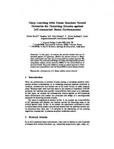
where the function h : R → R is L-Lipschitz continuous for some L < +∞, but is otherwise arbitrary (and so can be nonconvex). This family does not include the zero-one-loss (since it is not Lipschitz), but does include functions that can be used to approximate it to arbitrary accuracy with growing L. For instance, the piecewise-linear function: 1 x ≤ − 2L , 0 1 h(x) := 1 (3) x ≥ 2L , Lx + 1/2 otherwise, is L-Lipschitz, and converges to the step function as the parameter L increases to infinity. Shalev-Shwartz et al. (2011) study the problem of minimizing the objective (2) with function h defined by (3), and show that under a certain cryptographic assumption, there is no poly(L)-time algorithm for (approximate) minimization. Thus, it is reasonable to assume that the Lipschitz parameter L is a constant that does not grow with the dimension d or sample size n. Moreover, when f is a linear mapping, scaling the input vector x or scaling the weight vector w is equivalent to scaling the Lipschitz constant. Thus, we assume without loss of generality that the norms of x and w are bounded by one.
1.1
Our contributions
The first contribution of this paper is to present two poly(n, d)-time methods—namely, Algorithm 1 and Algorithm 2—for minimizing the cost function (2) for an arbitrary L-Lipschitz function h. We prove that for any given tolerance � > 0, these algorithms achieve an �-excess risk by running multiple rounds of random initialization followed by a constant number of optimization rounds (e.g., using an algorithm such as stochastic gradient descent). The first algorithm is based on choosing the initial vector uniformly at random from the Euclidean sphere; despite the simplicity of this scheme, it still has non-trivial guarantees. The second algorithm makes use a better initialization obtained by solving a least-squares problem, thereby leading to a stronger theoretical guarantee. Random initialization is a widely used heuristic in non-convex ERM; our analysis supports this usage but suggests that a careful theoretical treatment of the initialization step is necessary. Our algorithms for learning halfspaces have running time that grows polynomially in the pair (n, d), as well as a term proportional to exp((L/�2 ) log(L/�)). Our next contribution is to show that under a standard complexity-theoretic assumption—namely, that RP 6= NP—this exponential dependence on L/� cannot be avoided. More precisely, letting h denote the piecewise linear function from equation (3) with L = 1, Proposition 1 shows that there is no algorithm achieving arbitrary excess risk � > 0 in poly(n, d, 1/�) time when RP 6= NP. Thus, the random initialization scheme is unlikely to be substantially improved. 2
We then extend our approach to the learning of multi-layer neural networks, with a detailed analysis of the family of m-layer sigmoid-activated neural networks, under the assumption that `1 -norm of the incoming weights of any neuron is assumed to be bounded by a constant B. We specify a method (Algorithm 3) for training networks over this family, and in Theorem 3, we prove that its loss is at most an additive term of � worse than that of the best neural network. The time complexity of the algorithm scales as poly(n, d, Cm,B,1/� ), where the constant Cm,B,1/� does not depends on the input dimension or the data size, but may depend exponentially on the triplet (m, B, 1/�). Due to the exponential dependence on 1/�, this agnostic learning algorithm is too expensive to achieve a diminishing excess risk for a general data set. However, by analyzing data sets that are separable by some neural network with constant margin γ > 0, we obtain a stronger achievability result. In particular, we show in Theorem 4 that there is an efficient algorithm that correctly classifies all training points with margin Ω(γ) in polynomial time. As a consequence, the algorithm learns a neural network with generalization error bounded by � using poly(d, 1/�) training points and in poly(d, 1/�) time. This so-called BoostNet algorithm uses the AdaBoost approach (Freund and Schapire, 1997) to construct a m-layer neural network by taking an (m − 1)-layer network as a weak classifier. The shallower networks are trained by the agnostic learning algorithms that we develop in this paper. We establish the same learnability result when the labels are randomly flipped with probability η < 1/2 (see Corollary 1). Although the time complexity of BoostNet is exponential in 1/γ, we demonstrate that our achievable result is unimprovable—in particular, by showing that a poly(d, 1/�, 1/γ) complexity is impossible under a certain cryptographic assumption (see Proposition 2). Finally, we report experiments on learning parity functions with noise, which is a challenging problem in computational learning theory. We train two-layer neural networks using BoostNet, then compare them with the traditional backpropagation approach. The experiment shows that BoostNet learns the degree-5 parity function by constructing 50 hidden neurons, while the backpropagation algorithm fails to outperform random guessing.
1.2
Related Work
This section is devoted to discussion of some related work so as to put our contributions into broader context. 1.2.1
Learning halfspaces
The problem of learning halfspaces is an important problem in theoretical computer science. It is known that for any constant approximation ratio, the problem of approximately minimizing the zero-one loss is computationally hard (Guruswami and Raghavendra, 2009; Daniely et al., 2014). Halfspaces can be efficiently learnable if the data are drawn from certain special distributions, or if the label is corrupted by particular forms of noise. Indeed, Blum et al. (1998) and Servedio and Valiant (2001) show that if the labels are corrupted by random noise, then the halfspace can be learned in polynomial time. The same conclusion was established by Awasthi et al. (2015) when the labels are corrupted by Massart noise, and the covariates are drawn from the uniform distribution on a unit sphere. When the label noise is adversarial, the halfspace can be learned if the data distribution is isotropic log-concave and the fraction of labels being corrupted is bounded by a small quantity (Kalai et al., 2008; Klivans et al., 2009; Awasthi et al., 2014). When no assumption is made 3
on the noise, Kalai et al. (2008) show that if the data are drawn from the uniform distribution on a unit sphere, then there is an algorithm whose time complexity is polynomial in the input dimension, but exponential in 1/� (where � is the additive error). In this same setting, Klivans and Kothari (2014) prove that the exponential dependence on 1/� is unavoidable. Another line of work modifies the loss function to make it easier to minimize. Ben-David and Simon (2001) suggest comparing the zero-one loss of the learned halfspace to the optimal µ-margin loss. The µ-margin loss asserts that all points whose classification margins are smaller than µ should be marked as misclassified. Under this metric, it was shown by Ben-David and Simon (2001); Birnbaum and Shwartz (2012) that the optimal µ-margin loss can be achieved in polynomial time if µ is a positive constant. Shalev-Shwartz et al. (2011) study the minimization of a continuous approximation to the zero-one loss, which is similar to our setup. They propose a kernel-based algorithm which performs as well as the best linear classifier. However, it is an improper learning method in that the classifier cannot be represented by a halfspace. 1.2.2
Learning neural networks
It is known that any smooth function can be approximated by a neural network with just one hidden layer (Barron, 1993), but that training such a network is NP-hard (Blum and Rivest, 1992). In practice, people use optimization algorithms such as stochastic gradient (SG) to train neural networks. Although strong theoretical results are available for SG in the setting of convex objective functions, there are few such results in the nonconvex setting of neural networks. Several recent papers address the challenge of establishing polynomial-time learnability results for neural networks. Arora et al. (2013) study the recovery of denoising auto-encoders. They assume that the top-layer values of the network are randomly generated and all network weights are randomly drawn from {−1, 1}. As a consequence, the bottom layer generates a sequence of random observations from which the algorithm can recover the network weights. The algorithm has polynomial-time complexity and is capable of learning random networks that are drawn from a specific distribution. However, in practice people want to learn deterministic networks that encode data-dependent representations. Sedghi and Anandkumar (2014) study the supervised learning of neural networks under the assumption that the score function of the data distribution is known. They show that if the input dimension is large enough and the network is sparse enough, then the first network layer can be learned by a polynomial-time algorithm. More recently, Janzamin et al. (2015) propose another algorithm relying on the score function that removes the restrictions of Sedghi and Anandkumar (2014). The assumption in this case is that the network weights satisfy a non-degeneracy condition; however, the algorithm is only capable of learning neural networks with one hidden layer. Our algorithm does not impose any assumption on the data distribution, and is able to learn multilayer neural networks. Another approach to the problem is via the improper learning framework. The goal in this case is to find a predictor that is not a neural network, but performs as well as the best possible neural network in terms of the generalization error. Livni et al. (2014) propose a polynomial-time algorithm to learn networks whose activation function is quadratic. Zhang et al. (2015) propose an algorithm for improper learning of sigmoidal neural networks. The algorithm runs in poly(n, d, 1/�) time if the depth of the networks is a constant and the `1 -norm of the incoming weights of any node is bounded by a constant. It outputs a kernel-based classifier while our algorithm outputs a proper neural network. On the other hand, in the agnostic setting, the time complexity of our 4
0.5
0 -2
1
h(x)
1
h(x)
h(x)
1
0.5
0 0 value of x
(a) Step function
2
-2
0.5
0 0 value of x
2
(b) Piecewise linear function
-2
0 value of x
2
(c) Sigmoid function
Figure 1: Comparing the step function (panel (a)) with its two continuous approximations (panels (b) and (c)). algorithm depends exponentially on 1/�.
2
Preliminaries
In this section, we formalize the problem set-up and present several preliminary lemmas that are useful for the theoretical analysis. We first set up some notation so as to define a general empirical risk minimization problem. Let D be a dataset containing n points {(xi , yi )}ni=1 where xi ∈ X ⊂ Rd and yi ∈ {−1, 1}. To goal is to learn a function f : X → R so that f (xi ) is as close to yi as possible. We may write the loss function as `(f ) :=
n X
αi h(−yi f (xi )).
(4)
i=1
where hi : R → R is a L-Lipschitz continuous function that depends on yi , and {α1 , . . . , αn } are non-negative importance weights that sum to 1. As concrete examples, the function h can be the piecewise linear function defined by equation (3) or the sigmoid function h(x) := 1/(1 + e−4Lx ). Figure 1 compares the step function I[x ≥ 0] with these continuous approximations. In the following sections, we study minimizing the loss function in equation (4) when f is either a linear mapping or a multi-layer neural network. Let us introduce some useful shorthand notation. We use [n] to denote the set P of indices {1, 2, . . . , n}. For q ∈ [1, ∞], let kxkq denote the `q -norm of vector x, given by kxkq := ( dj=1 xqj )1/q , as well as kqk∞ = max |xj |. If u is a d-dimensional vector and σ : R → R is a function, we use j=1,...,d
σ(u) as a convenient shorthand for the vector (σ(u1�), . . . , σ(ud )). Given a class F of real-valued functions, we define the new function class σ ◦ F := σ ◦ f | f ∈ F . Rademacher complexity bounds: Let {(x0j , yj0 )}kj=1 be i.i.d. samples drawn from the dataset D such that probability of drawing (xi , yi ) is proportional to αi . We define the sample-based loss function: G(f ) :=
k 1X h(−yj0 f (x0j )). k j=1
5
(5)
It is straightforward to verify that E[G(f )] = `(f ). For a given function class F, the Rademacher complexity of F with respect to these k samples is defined as k h i 1X Rk (F) := E sup εj f (x0j ) , f ∈F k
(6)
j=1
where the {εj } are independent Rademacher random variables. Lemma 1. Assume that F contains the constant zero function f (x) ≡ 0, then we have h i E sup |G(f ) − `(f )| ≤ 4LRk (F). f ∈F
This lemma shows that Rk (F) controls the distance between G(f ) and `(f ). For the function classes √ studied in this paper, we will have Rk (F) = O(1/ k). Thus, the function G(f ) will be a good approximation to `(f ) if the sample size is large enough. This lemma is based on a slight sharpening of the usual Ledoux-Talagrand contraction for Rademacher variables (Ledoux and Talagrand, 2013); see Appendix A for the proof. Johnson-Lindenstrauss lemma: The Johnson-Lindenstrauss lemma is a useful tool for dimension reduction. It gives a lower bound on an integer s such that after projecting n vectors from a high-dimensional space into an s-dimensional space, the pairwise distances between this collection of vectors will be approximately preserved. Lemma 2. For any 0 < � < 1/2 and any positive integer n, consider any positive integer d s ≥ 12 log n/�2 . Let φ be a operator subspace p that projects a vector in R to a random s-dimensional d of R , then scales the vector by d/s. Then for any set of vectors u1 , . . . , un ∈ Rd , we have (7) kui − uj k22 − kφ(ui ) − φ(uj )k22 ≤ �kui − uj k22 for every i, j ∈ [n]. holds with probability at least 1/n. See the paper by Dasgupta and Gupta (1999) for a simple proof. Maurey-Barron-Jones lemma: Letting G be a subset of any Hilbert space H, the MaureyBarron-Jones lemma guarantees that any point v in the convex hull of G can be approximated by a convex combination of a small number of points of G. More precisely, we have: Lemma 3. Consider any subset G of any Hilbert space such that kgkH ≤ b for all g ∈ G. Then for any point v is in the convex hull of G, there is a point vs in the convex hull of s points of G such that kv − vs k2H ≤ b2 /s. See the paper by Pisier (1980) for a proof. This lemma is useful in our analysis of neural network learning.
6
Algorithm 1: Learning halfspaces based on initializing from uniform sampling Input: Feature-label pairs {(xi , yi )}ni=1 ; feature dimension d; parameters T and r ≥ 1. For t = 1, 2, . . . , T : 1. Draw a random vector u uniformly from the unit sphere of Rd . 2. Choose wt := ru, or compute wt by a poly(n, d)-time algorithm such that kwt k2 ≤ r and `(wt ) ≤ `(ru). Output: w b := arg minw∈{w1 ,...,wT } `(w).
3
Learning Halfspaces
In this section, we assume that the function f is a linear mapping f (x) := hw, xi, so that our cost function can be written as `(w) :=
n X
αi h(−yi hw, xi i).
(8)
i=1
In this section, we present two polynomial-time algorithms to approximately minimize this cost function over certain types of `p -balls. Both algorithms run multiple rounds of random initialization followed by arbitrary optimization steps. The first algorithm initializes the weight vector by uniformly drawing from a sphere. We next present and analyze a second algorithm in which the initialization follows from the solution of a least-square problem. It attains the stronger theoretical guarantees promised in the introduction.
3.1
Initialization by uniform sampling
We first analyze a very simple algorithm based on uniform sampling. Letting w∗ denote a minimizer of the objective function (8), by rescaling as necessary, we may assume that kw∗ k2 = 1. As noted earlier, by redefining the function h as necessary, we may also assume that the points {xi }ni=1 all lie inside the Eulcidean ball of radius one—that is, kxi k2 ≤ 1 for all i ∈ [n]. Given this set-up, a simply way in which to estimate w∗ is to first draw w uniformly from the Euclidean unit sphere, and then apply an iterative scheme to minimize the the loss function with the randomly drawn vector w as the initial point. At an intuitive level, this algorithm will find the global optimum if the initial weight is drawn sufficiently close to w∗ , so that the iterative optimization method converges to the global minimum. However, by calculating volumes of spheres in high-dimensions, it could require Ω( �1d ) rounds of random sampling before drawing a vector that is sufficiently close to w∗ , which makes it computationally intractable unless the dimension d is small. In order to remove the exponential dependence, Algorithm 1 is based on drawing the initial vector from a sphere of radius r > 1, where the radius r should be viewed as hyper-parameter of the algorithm. One should choose a greater r for a faster algorithm, but with a less accurate solution. The following theorem characterizes the trade-off between the accuracy and the time complexity.
7
Algorithm 2: Learning halfspaces based on initializing from the solution of a least-squares problem. Input: Feature-label pairs {(xi , yi )}ni=1 ; feature dimension d; parameters k, T . For t = 1, 2, . . . , T : 1. Sample k points {(x0j , yj0 )}kj=1 from the dataset with respect to their importance weights. P Sample a vector u uniformly from [−1, 1]k and let v := argminkwkp ≤1 kj=1 (hw, x0j i − uj )2 . 2. Choose wt := v, or compute wt by a poly(n, d)-time algorithm such that kwt kp ≤ 1 and `(wt ) ≤ `(v). Output: w b := arg minw∈{w1 ,...,wT } `(w). p Theorem 1. For 0 < � < 1/2 and δ > 0, let s := min{d, d12 log(n + 2)/�2 e}, r := d/s and T := d(2n + 4)(π/�)s−1 log(1/δ)e. With probability at least 1 − δ, Algorithm 1 outputs a vector kwk b 2 ≤ r which satisfies: `(w) b ≤ `(w∗ ) + 6�L. 2 ) log2 (1/�)
The time complexity is bounded by poly(n(1/�
, d, log(1/δ)).
The proof of Theorem 1, provided in Appendix B, uses the Johnson-Lindenstrauss lemma. More specifically, suppose that we project the weight vector w and all data points x1 , . . . , xn to a random subspace S and properly scale the projected vectors. The Johnson-Lindenstrauss lemma then implies that with a constant probability, the inner products hw, xi i will be almost invariant after the projection—that is, hw∗ , xi i ≈ hφ(w∗ ), φ(xi )i = hrφ(w∗ ), xi i
for every i ∈ [n],
where r is the scale factor of the projection. As a consequence, the vector rφ(w∗ ) will approximately minimize the loss. If we draw a vector v uniformly from the sphere of S with radius r and find that v is sufficiently close to rφ(w∗ ), then we call this vector v as a successful draw. The probability of a successful draw depends on the dimension of S, independent of the original dimension d (see Lemma 2). If the draw is successful, then we use v as the initialization so that it approximately minimize the loss. Note that drawing from the unit sphere of a random subspace S is equivalent to directly drawing from the original space Rd , so that there is no algorithmic need to explicitly construct the random subspace. It is worthwhile to note some important deficiencies of Algorithm 1. First, the algorithm outputs a vector satisfying the bound kwk b 2 ≤ r with r > 1, so that it is not guaranteed to lie within the Euclidean unit ball. Second, the `2 -norm constraints kxi k2 ≤ 1 and kw∗ k2 = 1 cannot 2 2 be generalized to other norms. Third, the complexity term n(1/� ) log (1/�) has a power growing with 1/�. Our second algorithm overcomes these limitations.
3.2
Initialization by solving a least-square problem
We turn to a more general setting in which w∗ and xi are bounded by a general `q -norm for some q ∈ [2, ∞]. Letting p ∈ [1, 2] denote the associated dual exponent ( i.e., such that 1/p + 1/q = 1), we assume that kw∗ kp ≤ 1 and kxi kq ≤ 1 for every i ∈ [n]. Note that this generalizes our previous 8
set-up, which applied to the case p = q = 2. In this setting, Algorithm 2 is a procedure that outputs an approximate minimizer of the loss function. In each iteration, it draws k � n points from the data set D, and then constructs a random least-squares problem based on these samples. The solution to this problem is used to initialize an optimization step. The success of Algorithm 2 relies on the following observation: if we sample k points independently from the dataset, then Lemma 1 implies that the sample-based loss G(f ) will be sufficiently close to the original loss `(f ). Thus, it suffices to minimize the sample-based loss. Note that G(f ) is uniquely determined by the k inner products ϕ(w) := (hw, xi1 i, . . . , hw, xik i). If there is a vector w satisfying ϕ(w) = ϕ(w∗ ), then its performance on the sample-based loss will be equivalent to that of w∗ . As a consequence, if we draw a vector u ∈ [−1, 1]k that is sufficiently close to ϕ(w∗ ) (called a successful u), then we can approximately minimize the sample-based loss by solving ϕ(w) = u, or alternatively by minimizing kϕ(w) − uk22 . The latter problem can be solved by a convex program in polynomial time. The probability of drawing a successful u only depends on k, independent of the input dimension and the sample size. This allows the time complexity to be polynomial in (n, d). The trade-off between the target excess risk and the time complexity is characterized by the following theorem. For given �, δ > 0, it is based on running Algorithm 2 with the choices ( d2 log d/�2 e if p = 1 k := (9) d(q − 1)/�2 e if p > 1, and T := d5(4/�)k log(1/δ)e. Theorem 2. For given �, δ > 0, with the choices of (k, T ) given above, Algorithm 2 outputs a vector kwk b p ≤ 1 such that `(w) b ≤ `(w∗ ) + 11�L
with probability at least 1 − δ.
The time complexity is bounded by ( � 2 poly n, d(1/� ) log(1/�) , log(1/δ) � 2 poly n, d, e(q/� ) log(1/�) , log(1/δ)
if p = 1 if p > 1.
See Appendix C for the proof. Theorem 2 shows that the time complexity of the algorithm has polynomial dependence on (n, d) but exponential dependence on L/�. Shalev-Shwartz et al. (2011) proved a similar complexity bound when the function h takes the piecewise-linear form (3), but our algorithm applies to arbitrary continuous functions. We note that the result is interesting only when (L/�)2 � d, since otherwise the same time complexity can be achieved by a grid search of w∗ within the d-dimensional unit ball.
3.3
Hardness result
In Theorem 2, the time complexity has an exponential dependence on L/�. Shalev-Shwartz et al. (2011) show that the time complexity cannot be polynomial in L even for improper learning. It is natural to wonder if Algorithm 2 can be improved to have polynomial dependence on (n, d, 1/�) given that L = 1. In this section, we provide evidence that this is unlikely to be the case. To prove the hardness result, we reduce from the MAX-2-SAT problem, which is known to be NP-hard. In particular, we show that if there is an algorithm solving the minimization problem (8), then it also solves the MAX-2-SAT problem. Let us recall the MAX-2-SAT problem: 9
Definition (MAX-2-SAT). Given n literals {z1 , . . . , zn } and d clauses {c1 , . . . , cd }. Each clause is the conjunction of two arguments that may either be a literal or the negation of a literal ∗ . The goal is to determine the maximum number of clauses that can be simultaneously satisfied by an assignment. Since our interest is to prove a lower bound, it suffices to study a special case of the general minimization problem—namely, one in which kw∗ k2 ≤ 1 and kxi k2 ≤ 1, yi = −1 for any i ∈ [n]. The following proposition shows that if h is the piecewise-linear function with L = 1, then approximately minimizing the loss function is hard. See Appendix D for the proof. Proposition 1. Let h be the piecewise-linear function (3) with Lipschitz constant L = 1. Unless RP = NP† , there is no randomized poly(n, d, 1/�)-time algorithm computing a vector w b which satisfies `(w) b ≤ `(w∗ ) + � with probability at least 1/2. Proposition 1 provides a strong evidence that learning halfspaces with respect to a continuous sigmoidal loss cannot be done in poly(n, d, 1/�) time. We note that Hush (1999) proved a similar hardness result, but without the unit-norm constraint on w∗ and {xi }ni=1 . The non-convex ERM problem without a unit norm constraint is notably harder than ours, so this particular hardness result does not apply to our problem setup.
4
Learning Neural Networks
Let us now turn to the case in which the function f represents a neural network. Given two numbers p ∈ (1, 2] and q ∈ [2, ∞) such that 1/p+1/q = 1, we assume that the input vector satisfies kxi kq ≤ 1 for every i ∈ [n]. The class of m-layer neural networks is recursively defined in the following way. A one-layer neural network is a linear mapping from Rd to R, and we consider the set of mappings: N1 := {x → hw, xi : kwkp ≤ B}. For m > 1, an m-layer neural network is a linear combination of (m − 1)-layer neural networks activated by a sigmoid function, and so we define: d n o X Nm := x → wj σ(fj (x)) : d < ∞, fj ∈ Nm−1 , kwk1 ≤ B . j=1
In this definition, the function σ : R → [−1, 1] is an arbitrary 1-Lipschitz continuous function. At each hidden layer, we allow the number of neurons d to be arbitrarily large, but the per-unit `1 -norm must be bounded by a constant B. This regularization scheme has been studied by Bartlett (1998); Koltchinskii and Panchenko (2002); Bartlett and Mendelson (2003); Neyshabur et al. (2015). Assuming a constant `1 -norm bound might be restrictive for some applications, but without this norm constraint, the neural network class activated by any sigmoid-like or ReLU-like function is not efficiently learnable (Zhang et al., 2015, Theorem 3). On the other hand, the `1 -regularization imposes sparsity on the neural network. It is observed in practice that sparse neural networks ∗ In the standard MAX-2-SAT setup, each clause is the disjunction of two literals. However, any disjunction clause can be reduced to three conjunction clauses. In particular, a clause z1 ∨z2 is satisfied if and only if one of the following is satisfied: z1 ∧ z2 , ¬z1 ∧ z2 , z1 ∧ ¬z2 . † RP is the class of randomized polynomial-time algorithms.
10
Algorithm 3: Algorithm for learning neural networks Input: Feature-label pairs {(xi , yi )}ni=1 ; number of layers m; parameters k, s, T, B. For t = 1, 2, . . . , T : 1. Sample k points {(x0j , yj0 )}kj=1 from the dataset with respect to their importance weights. 2. Generate a neural network g ∈ Nm in the following recursive way: • If m = 1, then draw a vector from [−B, B]k . Let Pk u uniformly 0 v := arg minw∈Rd :kwkp ≤B j=1 (hw, xj i − uj )2 and return g : x → hv, xi. • If m > 1, then generate the (m − 1)-layer networks g1 , . . . , gs ∈ Nm−1 using this recursive program. Draw a vector u uniformly from [−B, B]k . Let k �X s �2 X wl σ(gl (x0j )) − uj v := arg min w∈Rs :kwk1 ≤B
and return g : x →
j=1
(10)
l=1
Ps
l=1 vl σ(gl (x)).
3. Choose ft := g, or compute ft by a poly(n, d)-time algorithm such that ft ∈ Nm and `(ft ) ≤ `(g). Output: fb := arg minf ∈{f1 ,...,fT } `(f ).
are capable of learning meaningful representations such as by convolutional neural networks, for instance. Moreover, it has been argued that sparse connectivity is a natural constraint that can lead to improved performance in practice (see, e.g. Thom and Palm, 2013).
4.1
Agnostic learning
In the agnostic setting, it is not assumed there exists a neural network that separates the data. Instead, our goal is to compute a neural network fb ∈ Nm that minimizes the loss function over the space of all given networks. Letting f ∗ ∈ Nm be the network that minimizes the empirical loss `, we now present and analyze a method (see Algorithm 3) that computes a network whose loss is at most � worse that that of f ∗ . We first state our main guarantee for this algorithm, before providing intuition. More precisely, for any �, δ > 0, the following theorem applies to Algorithm 3 with the choices: l m m k := dq/�2 e, s := d1/�2 e, T := 5(4/�)k(s −1)/(s−1) log(1/δ) . (11) Theorem 3. For given B ≥ 1 and �, δ > 0, with the choices of (k, s, T ) given above, Algorithm 3 outputs a predictor fb ∈ Nm such that `(fb) ≤ `(f ∗ ) + (2m + 9)�LB m
with probability at least 1 − δ. 2 )m
The computational complexity is bounded by poly(n, d, eq(1/�
(12)
log(1/�) , log(1/δ)).
We remark that if m = 1, then Nm is a class of linear mappings. Thus, Algorithm 2 can be viewed as a special case of Algorithm 3 for learning one-layer neural networks. See Appendix E for the proof of Theorem 3. 11
The intuition underlying Algorithm 3 is similar to that of Algorithm 2. Each iteration involves resampling k independent points from the dataset. By the Rademacher generalization bound, minimizing the sample-based loss G(f ) will approximately minimize the original loss `(f ). The value of G(f ) is uniquely determined by the vector ϕ(f ) := (f (x01 ), . . . , f (x0k )). As a consequence, if we draw u ∈ [−B, B]k sufficiently close to ϕ(f ∗ ), then a nearly-optimal neural network will be obtained by approximately solving ϕ(g) ≈ u, or equivalently ϕ(g) ≈ ϕ(f ∗ ). In general, directly solving the equation ϕ(g) ≈ u would be difficult even if the vector u were known. In particular, since our class Nm is highly non-linear, solving this equation cannot be On the other hand, suppose that we write f ∗ (x) = Ps reduced ∗to solving a convex program. ∗ l=1 wl σ(fl (x)) for some functions fl ∈ Nm . Then the problem becomes much easier if the ∗ 0 quantities σ(fl (xj )) are already known for every (j, l) ∈ [k] × [d]. With this perspective in mind, we can approximately solve the equation by minimizing k �X s X
min
w∈Rd :kwk1 ≤B
j=1
wl σ(fl∗ (x0j )) − uj
�2
.
(13)
l=1
Accordingly, suppose that we draw vectors a1 , . . . , as ∈ [−B, B]k such that each aj is sufficiently close to ϕ(fj∗ )—any such draw is called successful. We may then recursively compute (m − 1)layer networks g1 , . . . , gs by first solving the approximate equation ϕ(gl ) ≈ al , and then rewriting problem (13) as k �X s X
min
w∈Rd :kwk1 ≤B
j=1
wl σ(gl (x0j )) − uj
�2
.
l=1
This convex program matches the problem (10) in Algorithm 3. Note that the probability of a successful draw {a1 , . . . , as } depends on the dimension s. Although there is no constraint on the dimension of Nm , the Maurey-Barron-Jones lemma (Lemma 3) asserts that it suffices to choose s = O(1/�2 ) to compute an �-accurate approximation. We refer the reader to Appendix E for the detailed proof.
4.2
Learning with separable data
We turn to the case in which the data are separable with a positive margin. Throughout this section, we assume that the activation function of Nm is an odd function (i.e., σ(−x) = −σ(x)). We say that a given data set {(xi , yi )}ni=1 is separable with margin γ, or γ-separable for short, if there is a network f ∗ ∈ Nm such that yi f ∗ (xi ) ≥ γ for each i ∈ [n]. Given a distribution P over the space X × {−1, 1}, we say that it is γ-separable if there is a network f ∗ ∈ Nm such that yf ∗ (x) ≥ γ almost surely (with respect to P). Algorithm 4 learns a neural network on the separable data. It uses the AdaBoost approach (Freund and Schapire, 1997) to construct the network, and we refer to it as the BoostNet algorithm. In each iteration, it trains a weak classifier gbt ∈ Nm−1 with an error rate slightly better than random guessing, then adds the weak classifier to the strong classifier to construct an m-layer network. The weaker classifier is trained by Algorithm 3 (or by Algorithm 1 or Algorithm 2 if Nm−1 are one-layer networks). The following theorem provides guarantees for its performance when it is run for T :=
l 16B 2 log(n + 1) m γ2 12
Algorithm 4: The BoostNet algorithm Input: Feature-label pairs {(xi , yi )}ni=1 ; number of layers m ≥ 2; parameters δ, γ, T, B. Initialize f0 = 0 and b0 = 0. For t = 1, 2, . . . , T : P 1. Define Gt (g) := ni=1 αt,i σ(−yi g(xi )) where g ∈ Nm−1 and αt,i :=
e−yi σ(ft−1 (xi )) Pn −yi σ(ft−1 (xi )) . j=1 e
2. Compute gbt ∈ Nm−1 by Algorithm 3 such that Gt (b gt ) ≤
inf
g∈Nm−1
Gt (g) +
γ 2B
(14)
with probability at least 1 − δ/T ‡ . Let µt := max{− 12 , Gt (b g )}. t 1−µt t gt and bt = bt−1 + 12 log( 1+µ ) . 3. Set ft = ft−1 + 21 log( 1−µ 1+µt )b t Output: fb :=
B bT
fT .
iterations. The running time depends on a quantity Cm,B,1/γ that is a constant for any choice of the triple (m, B, 1/γ), but with exponential dependence on 1/γ. Theorem 4. With the above choice of T , the BoostNet algorithm achieves: (a) In-sample error: For any γ-separable dataset {(xi , yi )}ni=1 Algorithm 4 outputs a neural network fb ∈ Nm such that, γ yi fb(xi ) ≥ for every i ∈ [n], with probability at least 1 − δ. 16 The time complexity is bounded by poly(n, d, log(1/δ), Cm,B,1/γ ). (b) Generalization error: Given a data set consisting of n = poly(1/�, log(1/δ)) i.i.d. samples from any γ-separable distribution P, Algorithm 4 outputs a network fb ∈ Nm such that � � P sign(fb(x)) 6= y ≤ � with probability at least 1 − 2δ. (15) Moreover, the time complexity is bounded by poly(d, 1/�, log(1/δ), Cm,B,1/γ ). See Appendix F for the proof. The most technical work is devoted to proving part (a). The generalization bound in part (b) follows by combining part (a) with bounds on the Rademacher complexity of the network class, which then allow us to translate the in-sample error bound to generalization error in the usual way. It is worth comparing the BoostNet algorithm with the general algorithm for agnostic learning. In order to bound the generalization error by � > 0, the time complexity of Algorithm 3 will be exponential in 1/�. The same learnability results can be established even if the labels are randomly corrupted. Formally, for every pair (x, y) sampled from a γ-separable distribution, suppose that the learning algorithm actually receives the corrupted pair (x, ye), where ( y with probability 1 − η, ye = −y with probability η. ‡
We may choose the hyper-parameters of Algorithm 3 by equation (11), with the additive error � defined by γ/((4m + 10)LB m ). Theorem 3 guarantees that the error bound (14) holds with high probability.
13
Here the parameter η ∈ [0, 12 ) corresponds to the noise level. Since the labels are flipped, the BoostNet algorithm cannot be directly applied. However, we can use the improper learning algorithm of Zhang et al. (2015) to learn an improper classifier b h such that b h(x) = y with high probability, and then apply the BoostNet algorithm taking (x, b h(x)) as input. Doing so yields the following guarantee: Corollary 1. Assume that q = 2 and η < 1/2. For any constant (m, B), consider the neural network class Nm activated by σ(x) := erf(x)§ . Given a random dataset of size n = poly(1/�, 1/δ) for any γ-separable distribution, there is a poly(d, 1/�, 1/δ)-time algorithm that outputs a network fb ∈ Nm such that P(sign(fb(x)) 6= y) ≤ �
with probability at least 1 − δ.
See Appendix G for the proof.
4.3
Hardness result for γ-separable problems
Finally, we present a hardness result showing that the dependence on 1/γ is hard to improve. Our proof relies on the hardness of standard (nonagnostic) PAC learning of the intersection of halfspaces given in Klivans et al. (2006). More precisely, consider the family of halfspace indicator functions mapping X = {−1, 1}d to {−1, 1} given by H = {x → sign(wT x − b − 1/2) : x ∈ {−1, 1}d , b ∈ N, w ∈ Nd , |b| + kwk1 ≤ poly(d)}. Given a T -tuple of functions {h1 , . . . , hT } belonging to H, we define the intersection function ( 1 if h1 (x) = · · · = hT (x) = 1, h(x) = −1 otherwise, which represents the intersection of T half-spaces. Letting HT denote the set of all such functions, for any distribution on X , we want an algorithm taking a sequence of (x, h∗ (x)) as input where x is a sample from X and h∗ ∈ HT . It should output a function b h such that P(b h(x) 6= h∗ (x)) ≤ � with probability at least 1−δ. If there is such an algorithm whose sample complexity and time complexity scale as poly(d, 1/�, 1/δ), then we say that HT is efficiently learnable. Klivans et al. (2006) show that if T = Θ(dρ ) then HT is not efficiently learnable under a certain cryptographic assumption. This hardness statement implies the hardness of learning neural networks with separable data. Proposition 2. Assume HT is not efficiently learnable for T = Θ(dρ ). Consider the class of twolayer neural networks N2 activated by the piecewise linear function σ(x) := min{1, max{−1, x}} or the ReLU function σ(x) := max{0, x}, and with the norm constraint B = 2. Consider any algorithm such that when applied to any γ-separable data distribution, it is guaranteed to output a neural network fb satisfying P(sign(fb(x)) 6= y) ≤ � with probability at least 1 − δ. Then it cannot run in poly(d, 1/�, 1/δ, 1/γ)-time. See Appendix H for the proof. § The erf function can be replaced by any function σ satisfying polynomial expansion σ(x) = P∞ j 2 2j < +∞ for any finite λ ∈ R+ . j=0 2 βj λ
14
P∞
j=0
βj xj , such that
0.5
BoostNet BackProp
prediction error
prediction error
0.5 0.4 0.3 0.2 0.1
BoostNet BackProp
0.4 0.3 0.2 0.1
0
5
10
15
20
0
number of hidden nodes
50
100
number of hidden nodes
(a) parity degree p = 2
(b) parity degree p = 5
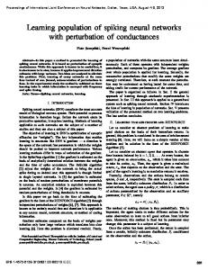
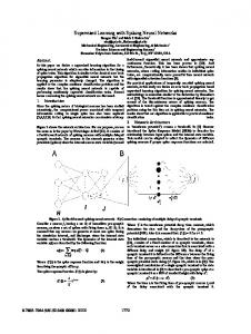
Figure 2: Performance of BoostNet and BackProp on the problem of learning parity function with noise.
5
Simulation
In this section, we compare the BoostNet algorithm with the classical backpropagation method for training two-layer neural networks. The goal is to learn parity functions from noisy data — a challenging problem in computational learning theory (see, e.g. Blum et al., 2003). We construct a synthetic dataset with n = 50, 000 points. Each point (x, y) is generated as follows: first, the vector x is uniformly drawn from {−1, 1}d and concatenated with a constant 1 as the (d+1)-th coordinate. The label is generated as follows: for some unknown subset of p indices 1 ≤ i1 < · · · < ip ≤ d, we set ( xi1 xi2 . . . xip with probability 0.9 , y= −xi1 xi2 . . . xip with probability 0.1 . The goal is to learn a function f : Rd+1 → R such that sign(f (x)) predicts the value of y. The optimal rate is achieved by the parity function f (x) = xi1 xi2 . . . xip , in which case the prediction error is 0.1. If the parity degree p > 1, the optimal rate cannot be achieved by any linear classifier. Choose d = 50 and p ∈ {2, 5}. The activation function is chosen as σ(x) := tanh(x). The training set, the validation set and the test set contain respectively 25K, 5K and 20K points. To train a two-layer BoostNet, we choose the hyper-parameter B = 10, and select Algorithm 3 as the subroutine to train weak classifiers with hyper-parameters (k, T ) = (10, 1). To train a classical two-layer neural network, we use the random initialization scheme of Nguyen and Widrow (1990) and the backpropagation algorithm of Møller (1993). For both methods, the algorithm is executed for ten independent rounds to select the best solution. Figure 5 compares the prediction errors of BoostNet and backpropagation. Both methods generate the same two-layer network architecture, so that we compare with respect to the number of hidden nodes. Note that BoostNet constructs hidden nodes incrementally while NeuralNet trains a predefined number of neurons. Figure 5 shows that both algorithms learn the degree-2 parity function with a few hidden nodes. In contrast, BoostNet learns the degree-5 parity function with less than 50 hidden nodes, while NeuralNet’s performance is no better than random guessing. This suggests that the BoostNet algorithm is less likely to be trapped in a bad local optimum in this setting. 15
6
Conclusion
In this paper, we have proposed algorithms to learn halfspaces and neural networks with non-convex loss functions. We demonstrate that the time complexity is polynomial in the input dimension and in the sample size but exponential in the excess risk. A hardness result relating to the necessity of the exponential dependence is also presented. The algorithms perform randomized initialization followed by optimization steps. This idea coincides with the heuristics that are widely used in practice, but the theoretical analysis suggests that a careful treatment of the initialization step is necessary. We proposed the BoostNet algorithm, and showed that it can be used to learn a neural network in polynomial time when the data are separable with a constant margin. We suspect that the theoretical results of this paper are likely conservative, in that in application to real data, the algorithms can be much more efficient than the bounds might suggest.
Acknowledgements: MW and YZ were partially supported by NSF grant CIF-31712-23800 from the National Science Foundation, AFOSR-FA9550-14-1-0016 grant from the Air Force Office of Scientific Research, ONR MURI grant N00014-11-1-0688 from the Office of Naval Research. MJ and YZ were partially supported by the U.S.ARL and the U.S.ARO under contract/grant number W911NF-11-1-0391. We thank Sivaraman Balakrishnan for helpful comments on an earlier draft.
References S. Arora, A. Bhaskara, R. Ge, and T. Ma. Provable bounds for learning some deep representations. arXiv:1310.6343, 2013. P. Awasthi, M. F. Balcan, and P. M. Long. The power of localization for efficiently learning linear separators with noise. In Proceedings of the 46th Annual ACM Symposium on Theory of Computing, pages 449–458. ACM, 2014. P. Awasthi, M.-F. Balcan, N. Haghtalab, and R. Urner. Efficient learning of linear separators under bounded noise. arXiv:1503.03594, 2015. A. R. Barron. Universal approximation bounds for superpositions of a sigmoidal function. IEEE Transactions on Information Theory, 39(3):930–945, 1993. P. L. Bartlett. The sample complexity of pattern classification with neural networks: the size of the weights is more important than the size of the network. Information Theory, IEEE Transactions on, 44(2):525–536, 1998. P. L. Bartlett and S. Mendelson. Rademacher and gaussian complexities: Risk bounds and structural results. The Journal of Machine Learning Research, 3:463–482, 2003. S. Ben-David and H. U. Simon. Efficient learning of linear perceptrons. In Advances in Neural Information Processing Systems, volume 13, page 189. MIT Press, 2001. A. Birnbaum and S. S. Shwartz. Learning halfspaces with the zero-one loss: time-accuracy tradeoffs. In Advances in Neural Information Processing Systems, volume 24, pages 926–934, 2012. 16
A. Blum and R. L. Rivest. Training a 3-node neural network is NP-complete. Neural Networks, 5 (1):117–127, 1992. A. Blum, A. Frieze, R. Kannan, and S. Vempala. A polynomial-time algorithm for learning noisy linear threshold functions. Algorithmica, 22(1-2):35–52, 1998. A. Blum, A. Kalai, and H. Wasserman. Noise-tolerant learning, the parity problem, and the statistical query model. Journal of the ACM, 50(4):506–519, 2003. A. Daniely, N. Linial, and S. Shalev-Shwartz. From average case complexity to improper learning complexity. In Proceedings of the 46th Annual ACM Symposium on Theory of Computing, pages 441–448. ACM, 2014. S. Dasgupta and A. Gupta. An elementary proof of the Johnson-Lindenstrauss lemma. International Computer Science Institute, Technical Report, pages 99–006, 1999. Y. Freund and R. E. Schapire. A decision-theoretic generalization of on-line learning and an application to boosting. Journal of Computer and System Sciences, 55(1):119–139, 1997. V. Guruswami and P. Raghavendra. Hardness of learning halfspaces with noise. SIAM Journal on Computing, 39(2):742–765, 2009. D. R. Hush. Training a sigmoidal node is hard. Neural Computation, 11(5):1249–1260, 1999. M. Janzamin, H. Sedghi, and A. Anandkumar. Generalization bounds for neural networks through tensor factorization. arXiv:1506.08473, 2015. S. Kakade and A. Tewari. Lecture note: Rademacher composition and linear prediction. 2008. S. M. Kakade, K. Sridharan, and A. Tewari. On the complexity of linear prediction: Risk bounds, margin bounds, and regularization. In Advances in Neural Information Processing Systems, volume 21, pages 793–800, 2009. A. T. Kalai, A. R. Klivans, Y. Mansour, and R. A. Servedio. Agnostically learning halfspaces. SIAM Journal on Computing, 37(6):1777–1805, 2008. A. Klivans and P. Kothari. Embedding hard learning problems into gaussian space. Approximation, Randomization, and Combinatorial Optimization. Algorithms and Techniques, 28:793–809, 2014. A. R. Klivans, A. Sherstov, et al. Cryptographic hardness for learning intersections of halfspaces. In 47th Annual IEEE Symposium on Foundations of Computer Science, pages 553–562. IEEE, 2006. A. R. Klivans, P. M. Long, and R. A. Servedio. Learning halfspaces with malicious noise. The Journal of Machine Learning Research, 10:2715–2740, 2009. V. Koltchinskii and D. Panchenko. Empirical margin distributions and bounding the generalization error of combined classifiers. Annals of Statistics, pages 1–50, 2002. M. Ledoux and M. Talagrand. Probability in Banach Spaces: isoperimetry and processes, volume 23. Springer Science & Business Media, 2013. 17
R. Livni, S. Shalev-Shwartz, and O. Shamir. On the computational efficiency of training neural networks. In Advances in Neural Information Processing Systems, volume 26, pages 855–863, 2014. M. F. Møller. A scaled conjugate gradient algorithm for fast supervised learning. Neural networks, 6(4):525–533, 1993. B. Neyshabur, R. Tomioka, and N. Srebro. Norm-based capacity control in neural networks. arXiv preprint arXiv:1503.00036, 2015. D. Nguyen and B. Widrow. Improving the learning speed of 2-layer neural networks by choosing initial values of the adaptive weights. In International Joint Conference on Neural Networks, pages 21–26, 1990. G. Pisier. Remarques sur un r´esultat non publi´e de B. Maurey. S´eminaire Analyse Fonctionnelle, pages 1–12, 1980. F. Rosenblatt. The perceptron: a probabilistic model for information storage and organization in the brain. Psychological Review, 65(6):386, 1958. R. E. Schapire and Y. Singer. Improved boosting algorithms using confidence-rated predictions. Machine Learning, 37(3):297–336, 1999. H. Sedghi and A. Anandkumar. Provable methods for training neural networks with sparse connectivity. arXiv:1412.2693, 2014. R. Servedio and L. Valiant. Efficient algorithms in computational learning theory. Harvard University, Cambridge, MA, 2001. S. Shalev-Shwartz and Y. Singer. On the equivalence of weak learnability and linear separability: New relaxations and efficient boosting algorithms. Machine Learning, 80(2-3):141–163, 2010. S. Shalev-Shwartz, O. Shamir, and K. Sridharan. Learning kernel-based halfspaces with the 0-1 loss. SIAM Journal on Computing, 40(6):1623–1646, 2011. M. Thom and G. Palm. Sparse activity and sparse connectivity in supervised learning. The Journal of Machine Learning Research, 14(1):1091–1143, 2013. V. N. Vapnik. Statistical learning theory, volume 1. Wiley New York, 1998. Y. Zhang, J. D. Lee, and M. I. Jordan. `1 -regularized neural networks are improperly learnable in polynomial time. arXiv:1510.03528, 2015.
A
Proof of Lemma 1
The following inequality always holds: sup |G(f ) − `(f )| ≤ max f ∈F
n
o sup {G(f ) − `(f )}, sup {`(f 0 ) − G(f 0 )} . f 0 ∈F
f ∈F
18
Since F contains the constant zero function, both supf ∈F {G(f ) − `(f )} and supf 0 ∈F {`(f 0 ) − G(f 0 )} are non-negative, which implies sup |G(f ) − `(f )| ≤ sup {G(f ) − `(f )} + sup {`(f 0 ) − G(f 0 )}. f ∈F
f 0 ∈F
f ∈F
To establish Lemma 1, it suffices to prove: h i E sup {G(f ) − `(f )} ≤ 2LRk (F) f ∈F
h i and E sup {`(f 0 ) − G(f 0 )} ≤ 2LRk (F) f 0 ∈F
For the rest of the proof, we will establish the first upper bound. The second bound can be established through an identical series of steps. The inequality E[supf ∈F {G(f ) − `(f )}] ≤ 2LRk (F) follows as a consequence of classical symmetrization techniques (e.g. Bartlett and Mendelson, 2003) and the Talagrand-Ledoux concentration (e.g. Ledoux and Talagrand, 2013, Corollary 3.17). However, so as to keep the paper self-contained, we provide a detailed proof here. By the definitions of `(f ) and G(f ), we have k k h n oi h n1 X h1 X ioi E sup G(f ) − `(f ) = E sup h(−yj0 f (x0j )) − E h(−yj00 f (x00j )) , k f ∈F f ∈F k j=1
j=1
where (x00j , yj00 ) is an i.i.d. copy of (x0j , yj0 ). Applying Jensen’s inequality yields k n oi h n1 X oi h h(−yj0 f (x0j )) − h(−yj00 f (x00j )) E sup G(f ) − `(f ) ≤ E sup f ∈F k f ∈F j=1
k h n1 X oi = E sup εj (h(−yj0 f (x0j )) − h(−yj00 f (x00j ))) f ∈F k j=1
k k h n1 X oi 1X ≤ E sup εj h(−yj0 f (x0j )) + sup εj h(−yj00 f (x00j )) f ∈F k f ∈F k j=1
j=1
k oi h n1 X εj h(−yj0 f (x0j )) . = 2E sup f ∈F k
(16)
j=1
We need to bound the right-hand side using the Rademacher complexity of the function class F, and we use an argument following the lecture notes of Kakade and Tewari (2008). Introducing the shorthand notation ϕj (x) := h(−yj0 x), the L-Lipschitz continuity of ϕj implies that k k h i h n ϕ (f (x0 )) − ϕ (f 0 (x0 )) X X ϕj (f (x0j )) + ϕj (f 0 (x0j )) oi 1 1 1 1 εj ϕj (f (x0j )) = E sup + εj E sup 2 2 f ∈F f,f 0 ∈F j=1
j=2
k h n L|f (x0 ) − f 0 (x0 )| X ϕj (f (x0j )) + ϕj (f 0 (x0j )) oi 1 1 ≤ E sup + εj 2 2 f,f 0 ∈F j=2
k h n Lf (x0 ) − Lf 0 (x0 ) X ϕj (f (x0j )) + ϕj (f 0 (x0j )) oi 1 1 = E sup + εj . 2 2 f,f 0 ∈F j=2
19
Applying Jensen’s inequality implies that the right-hand side is bounded by k k n o n oi X X 1 h 0 0 0 RHS ≤ E sup Lf (x1 ) + εj ϕj (f (xj )) + sup − Lf (x1 ) + εj ϕj (f 0 (x0j )) 2 f ∈F f 0 ∈F j=2
h n = E sup ε1 Lf (x01 ) +
k X
f ∈F
j=2
oi εj ϕj (f (x0j )) .
j=2
By repeating this argument for j = 2, 3, . . . , k, we obtain k k h i h i X X E sup εj ϕj (f (x0j )) ≤ LE sup εj f (x0j ) . f ∈F j=1
(17)
f ∈F j=1
Combining inequalities (16) and (17), we have the desired bound.
B
Proof of Theorem 1
Let us study a single iteration of Algorithm 1. Recall that u is uniformly sampled from the unit sphere of Rd . Alternatively, it can be viewed as sampled by the following procedure: first draw a random s-dimensional subspace of Rd , then draw u uniformly from the unit sphere of S. Consider the n + 2 fixed points {0, w∗ , x1 , . . . , xn }. Let φ(w) := rΠS (w) be an operator that projects the p vector w ∈ Rd to the subspace S and scale it by r. If we choose s ≥ 12 log(n+2) and r := d/s, 2 � then Lemma 2 implies that with probability at least 1/(n + 2), we are guaranteed that |kφ(w∗ )k22 | − kw∗ k22 | ≤ �,
kφ(xi )k22 | − kxi k22 | ≤ �
and
|kφ(w∗ ) − φ(xi )k22 − kw∗ − xi k22 | ≤ |4� for any i ∈ [n].
(18)
Consequently, we have |hφ(w∗ ), φ(xi )i − hw∗ , xi i| ≤ 3� for any i ∈ [n].
(19)
Assume that the approximation bounds (18) and (19) hold. Then using the L-Lipschitz continuity of h, we have `(w∗ ) =
n X
αi h(−yi hw∗ , xi i) ≥ −3�L +
i=1
k X
αi h(−yi hφ(w∗ ), φ(xi )i).
(20)
j=1
Recall that u is uniformly drawn from the unit sphere of S; therefore, the angle between u and φ(w∗ ) is at most � with probability at least (�/π)s−1 . By inequality (18), the norm of φ(w∗ ) is in [1 − �, 1 + �]. Hence, whenever the angle bound holds, the distance between u and φ(w∗ ) is bounded by 2�. Combining this bound with inequality (20), we find that `(w∗ ) ≥ −3�L +
n X
αi h(−yi hu + (φ(w∗ ) − u), φ(xi )i).
i=1
20
Note that we have the inequality |hφ(w∗ ) − u, φ(xi )i| ≤ kφ(w∗ ) − uk2 kφ(xi )k2 ≤ 2�(1 + �) ≤ 3�. Combined with the L-Lipschitz condition, we obtain the lower bound `(w∗ ) ≥ −6�L +
k X
αi h(−yi hu, φ(xi )i) = `(ru) − 6�L.
(21)
j=1 s−1
This bound holds with probability at least (�/π) 2n+4 . Thus, by repeating the procedure for a total s−1 of T ≥ (2n + 4)(π/�) log(1/δ) iterations, then the best solution satisfies inequality (21) with probability at least 1 − δ. The time complexity is obtained by plugging in the stated choices of (s, T ).
C
Proof of Theorem 2
Let us study a single iteration of Algorithm 2. Conditioning on any {(x0j , yj0 )}kj=1 , define the function P G(w) := k1 kj=1 h(−yj0 hw, x0j i). Since h is L-Lipschitz, we have G(v) − G(w∗ ) =
k k LX 1X h(−yj0 hv, x0j i) − h(−yj0 hw∗ , x0j i) ≤ |hv − w∗ , x0j i| k k j=1
j=1
k
�1/2 L �X ≤√ (hv − w∗ , x0j i)2 , k j=1 where the final step follows from the Cauchy-Schwarz inequality. Let X 0 ∈ Rk×d be a design matrix whose j-th row is equal to x0j . Using the above bound, for any u ∈ [−1, 1]k , we have L L G(v) − G(w∗ ) ≤ √ kX 0 (v − w∗ )k2 ≤ √ (kX 0 v − uk2 + kX 0 w∗ − uk2 ) k k 2L ≤ √ kX 0 w∗ − uk2 , k
(22)
where the last step uses the fact that the vector v minimizes kX 0 w − uk2 over the set of vectors with kwkp ≤ 1. The right-hand side of inequality (22) is independent of v. Indeed, since X 0 w∗ ∈ [−1, 1]k and u is uniformly sampled from this cube, √ the probability that kX 0 w∗ − uk∞ ≤ �/2 is at least k 0 ∗ (�/4) . This bound leads to kX w − uk2 ≤ � k/2. Thus, with probability at least (�/4)k , we have G(v) − G(w∗ ) ≤ �L. Conditioned on the above bound holding, Lemma 1 implies that h i E sup `(w) − G(w) ≤ 4LRk (F), kwkp ≤1
where Rk (F) is the k-sample Rademacher complexity of the function class F := {f : x → hw, xi | kwkp ≤ 1, kxkq ≤ 1}. Markov’s inequality implies that supkwkp ≤1 `(w) − G(w) ≤ 5LRk (F) with 21
probability at least 1/5. This event only depends on the choice of {(x0j , yj0 )}, and conditioned on it holding, we have `(v) ≤ G(v) + 5LRk (F) = G(w∗ ) + (G(v) − G(w∗ )) + 5LRk (F) ≤ `(f ∗ ) + (G(v) − G(w∗ )) + 10LRk (F). It is known (e.g. Kakade et al., 2009) that the Rademacher complexity is upper bounded as q 2 log d if p = 1 Rk (F) ≤ q k q−1 if p > 1, where 1/q + 1/p = 1. k Thus, given the choice of k from equation (9) and plugging in the bound on G(v) − G(w∗ ), we have `(v) ≤ `(w∗ ) + 11�L with probability at least (�/4)k /5. Repeating this procedure for a total of T ≥ 5(4/�)k log(1/δ) times guarantees that the upper bound holds with probability at least 1 − δ. Finally, the claimed time complexity is obtained by plugging in the stated choices of k and T .
D
Proof of Proposition 1
We prove the lower bound based on a data set with kxi k2 ≤ 1 and yi = −1 for each i ∈ [n]. With this set-up, consider the following problem: n
minimize `(w) s.t. kwk2 ≤ 1
where
`(w) :=
1X h(hw, xi i). n
(23)
i=1
The following lemma, proved in Appendix D.1, shows that for a specific 1-Lipschitz continuous function h, approximately minimizing the loss function is NP-hard. Lemma 4. Consider the optimization problem (23) based on the function h(x) := min{0, x}. It 1 is NP-hard to compute a vector w b ∈ Rd such that kwk b 2 ≤ 1 and `(w) b ≤ `(w∗ ) + (n+2)d . We reduce the problem described by Lemma 4 analyzing the piecewise linear function 1 h(x) := 0 x + 1/2
to the problem of Theorem 1. We do so by
x ≥ 1/2, x ≤ −1/2, otherwise.
(24)
With this choice of h, consider an instance of the problem underlying Lemma 4, say n
min g(w) :=
kwk2 ≤1
1X min{0, hw, xi i}, n
(25)
i=1
and let w∗ be a vector that achieves the above minimum. Our next step is to construct a new problem in dimension d+1, and argue that any approximate solution to it also leads to an approximate solution to √ √ the generic instance (25). For each i ∈ [n], √ define the (d + 1)-dimensional vector x0i := (xi / 2, 1/ 2), as well as the quantities u := −ed+1 / 2 22
√ and v := ed+1 /(2 2). Here ed+1 represents the unit vector aligning with the (d + 1)-th coordinate. For a (d + 1)-dimensional weight vector w e ∈ Rd+1 , consider the objective function n � X 1 � e `(w) e := 6nh(hw, e ui) + 6nh(hw, e vi) + h(hw, e x0i i) . 13n i=1
√ √ If we decompose w e as w e = (α/ 2, τ / 2) where α ∈ Rd and τ ∈ R, then these parameters satisfy kαk22 + τ 2 ≤ 2. We then have the equivalent expression n � X 1 � e w) `( e = 6nh(−τ /2) + 6nh(τ /4) + h(hα, xi i/2 + τ /2) . 13n i=1
1 Lemma 5. Given any � ∈ (0, 26 ), suppose that w e= ¶ function `e with additive error �, Then we have
g
α √τ √ , 2 2
�
is an approximate minimizer of the
� α � ≤ g(w∗ ) + 26�. kαk2
(26)
e then there is a polynomialThus, if there is a polynomial-time algorithm for minimizing function `, time algorithm for minimizing function g. Applying the hardness result for minimization of the function g (see Lemma 4) completes the proof of the proposition. It remains to prove the two lemmas, and we do so in the following two subsections.
D.1
Proof of Lemma 4
We reduce MAX-2-SAT to the minimization problem. Given a MAX-2-SAT instance, we construct a loss function ` so that if any algorithm computes a vector w b satisfying `(w) b ≤ `(w∗ ) +
1 , (2n + 2)d
then the vector w b solves MAX-2-SAT. First, we construct n + 1 vectors in Rd . Define the vector x0 := vectors xi :=
√1 x0 , d i
where
x0i
∈
Rd
(27)
√1 1d , d
and for i = 1, . . . , n, the
is given by
1 0 xij = −1 0
if zi appears in cj , if ¬zi appears in cj , otherwise.
It is straightforward to verify that that kxi k2 ≤ 1 for any i ∈ {0, 1, . . . , n}. We consider the following minimization problem: `(w) =
n � 1 X� min{0, hw, xi i} + min{0, hw, −xi i} . 2n + 2 i=0
¶
In making this claim, we define 0/k0k2 := 0.
23
The goal is to find a vector w∗ ∈ Rd such that kw∗ k2 ≤ 1 and it minimizes the function `(w). Notice that for every index i, at most one of min{0, hw, xi i} and min{0, hw, −xi i} is non-zero. Thus, we may write the minimization problem as min (2n + 2)`(w) = min
kwk2 ≤1
kwk2 ≤1
n � X i=0
min
� hw, αi xi i =
αi ∈{−1,1}
=
min
min
α∈{−1,1}n+1 kwk2 ≤1
n X
hw, αi xi i
i=0
n
X
min − αi xi n+1
α∈{−1,1}
= −
max
2
i=0
α∈{−1,1}n+1
d �X n X j=1
1/2 αi xij
�2
.
i=0
(28) P P We claim that maximizing dj=1 ( ni=0 αi xij )2 with respect to α is equivalent to maximizing the number of satisfiable clauses. In order to prove this claim, we consider an arbitrary assignment to α to construct a solution to the MAX-2-SAT problem. For i = 1, 2, . . . , n, let zi = true if αi = α0 , and let zi = false if αi = −α0 . With this assignment, it is straightforward to verify the following: √ √ Pn if the clause cj is satisfied, then the value of i=0 αi xij is√either 3/√d or −3/ d. If the clause is not satisfied, then the value of the expression is either 1/ d or −1/ d. To summarize, we have d �X n X j=1
αi xij
�2
=1+
i=0
8 × (# of satisfied clauses) . d
(29)
Thus, solving problem (28) determines the maximum number of satisfiable clauses: � �2 d� (max # of satisfied clauses) = min (2n + 2)`(w) − 1 . 8 kwk2 ≤1 By examining equation (28) and (29), we find that the value of (2n + 2)`(w) ranges in [−3, 0]. Thus, the MAX-2-SAT number is exactly determined if (2n + 2)`(w) b is at most 1/d larger than the optimal value. This optimality gap is guaranteed by inequality (27), which completes the reduction.
D.2
Proof of Lemma 5
In order to prove the claim, we first argue that τ ∈ [0, 2]. If this inclusion does not hold, then it 6 can be verified that h(−τ /2) + h(τ /4) ≥ 13 , which implies that n
6 1 X 12 e w) `( e ≥ + h(hα, xi i/2 + τ /2) ≥ . 13 13n 26 i=1
However, the feasible assignment (α, τ ) = (0, 1) achieves function value e w) assumption that `( e is �-optimal. Thus, we assume henceforth τ ∈ [0, 2], and we can rewrite `e as n
11 26 ,
1 X 3|τ − 1| + 9 e w) + h(hα, xi i/2 + τ /2). `( e = 26 13n i=1
24
which contradicts the
Notice that h(x + 1/2) is lower bounded by 1 + min{0, x}. Thus, we have the lower bound n
1 1 X 3|τ − 1| + 9 e w) + + `( e ≥ min{0, hα, xi i/2 + (τ − 1)/2} 26 13 13n i=1
11 g(α/2) |τ − 1| + + , (30) 26 13 13 where the last inequality uses the 1-Lipschitz continuous of min{0, x}. Notice that the function g satisfies g(βw) = βg(w) for any scalar β. Thus, we can further lower bound the right-hand side by kαk2 � α � 1 � α � max{0, kαk2 − 1} ≥ g − ·g , (31) g(α/2) = 2 kαk2 2 kαk2 2 ≥
α where the last inequality uses the fact that g( kαk ) ≥ −1. Note that inequality (31) holds even 2 for α = 0 according the definition that 0/k0k2 = 0. If the quantity kαk2 − 1 is positive, then kαk2 > 1 and consequently τ < 1. Thus we have
kαk2 − 1 < kαk22 − 1 ≤ 1 − τ 2 = (1 + τ )(1 − τ ) < 2(1 − τ ). α ) − |τ − 1|. Combining this bound with inequality (30), Thus, we can lower bound g(α/2) by 21 g( kαk 2 we obtain the lower bound 11 1 � α � `(w) e ≥ + g . (32) 26 26 kαk2
Note that the assignment (α, τ ) = (w∗ , 1) is feasible. For this assignment, it is straightforward 11 1 to verify that the function value is equal to 26 + 26 g(w∗ ). Using the fact that w e is an �-optimal 1 11 ∗ + g(w ) + �. This combining with inequality (32) implies that solution, we have `( w) e ≤ 26 26 � �
g
E
α kαk2
≤ g(w∗ ) + 26�, which completes the proof.
Proof of Theorem 3
Recalling the definition (6) of the Rademacher complexity, the following lemma bounds the complexity of Nm . q Lemma 6. The Rademacher complexity of Nm is bounded as Rk (Nm ) ≤ kq B m . See Appendix E.1 for the proof. We study a single iteration of Algorithm 3. Conditioning on any {(x0j , yj0 )}, define the quantity P G(f ) := k1 kj=1 h(−yj0 f (x0j )). Since the function h is L-Lipschitz continuous, we have h(−yj0 g(x0j )) − h(−yj0 f ∗ (x0j )) ≤ L|g(x0j ) − f ∗ (x0j )| for any j ∈ [k].
(33)
Given any function f : Rd → R, we denote the vector (f (x01 ), . . . , f (x0k )) by ϕ(f ). For inP stance, kϕ(g) − ϕ(f ∗ )k2 represents the `2 -norm ( kj=1 |g(x0j ) − f ∗ (x0j )|2 )1/2 . Inequality (33) and the Cauchy-Schwarz inequality implies k
G(g) − G(f ∗ ) ≤
LX L |g(x0j ) − f ∗ (x0j )| ≤ √ kϕ(g) − ϕ(f ∗ )k2 . k k j=1
We need one further auxiliary lemma: 25
Lemma 7. For any fixed function f ∗ ∈ Nm , we have √ kϕ(g) − ϕ(f ∗ )k2 ≤ (2m − 1)� kB m
with probability at least
pm :=
� � �k(sm −1)/(s−1) 4
.
(34)
See Appendix E.2 for the proof of this claim. Let us now complete the proof of the theorem, using this two lemmas. Lemma 1 implies that h i E sup `(f ) − G(f ) ≤ 4LRk (Nm ). f ∈Nm
By Markov’s inequality, we have supf ∈Nm `(f ) − G(f ) ≤ 5LRk (Nm ) with probability at least 1/5. This event only depends on the choice of {(x0j , yj0 )}. If it is true, then we have `(g) ≤ G(g) + 5LRk (Nm ) = G(f ∗ ) + (G(g) − G(f ∗ )) + 5LRk (Nm ) L ≤ `(f ∗ ) + √ kϕ(g) − ϕ(f ∗ )k2 + 10LRk (Nm ). k q Q 2 By Lemma 6, we have Rk (Nm ) ≤ kq m l=1 Bl . Thus, setting k = q/� , substituting the bound into equation (34) and simplifying yields `(g) ≤ `(f ∗ ) + (2m + 9)�LB m with probability at least pm /5. If we repeat the procedure for T = (5/pm ) log(1/δ) times, then the desired bound holds with probability at least 1 − δ. The time complexity is obtained by plugging in the choices of (s, k, T ).
E.1
Proof of Lemma 6
We prove the q claim by induction on the number of layers m. It is known (Kakade et al., 2009) that
Rk (N1 ) ≤ kq B. Thus, the claim holds for the base case m = 1. Now consider some m > 1, and assume that the claim holds for m − 1. We then have # " k 1X 0 Rk (N1 ) = E sup εi f (xi ) , f ∈Nm k i=1
where ε1 , . . . , εn are Rademacher variables. By the definition of Nm , we may write the expression as n d d k X X X X 1 1 Rk (N1 ) = E sup εi wj σ(fj (x0i )) = E sup wj εi σ(fj (x0i )) k f1 ,...,fd ∈Nm−1 k i=1 f ,...,f ∈N 1 m−1 d j=1 j=1 i=1 " # k 1X ≤ BE sup εi σ(f (x0i )) f ∈Nm−1 k i=1
= BRk (σ ◦ Nm−1 ), 26
where the inequality follows since kwk1 ≤ B. Since the function σ is 1-Lipschitz continuous, following the proof of inequality (17), we have r q m Rk (σ ◦ Nm−1 ) ≤ Rk (Nm−1 ) ≤ B , n which completes the proof.
E.2
Proof of Lemma 7
We prove the claim by induction on the number of layers m. If m = 1, then f ∗ is a linear function and ϕ(f ∗ ) ∈ [−B1 , B1 ]n . Since ϕ(g) minimizes the `2 -distance to vector u, we have kϕ(g) − ϕ(f ∗ )k2 ≤ kϕ(g) − uk2 + kϕ(f ∗ ) − uk2 ≤ 2kϕ(f ∗ ) − uk2 .
(35)
Since u is drawn uniformly from [−B, B]k , with probability at least ( 4� )k we have kϕ(f ∗ ) − uk∞ ≤ and consequently √ √ kϕ(g) − ϕ(f ∗ )k2 ≤ kkϕ(g) − ϕ(f ∗ )k∞ ≤ � kB,
�B 2 ,
which establishes the claim. ∗ For m > 1, assume that the claim holds for m − 1. Recall that √ f /B is in the convex hull of σ ◦ Nm−1 and every function f ∈ σ ◦ Nm−1 satisfies kϕ(f )k2 ≤ k. By the Maurey-Barron-Jones lemma (Lemma 3), there exist s functions in Nm−1 , say fe1 , . . . , fes , and a vector w ∈ Rs satisfying kwk1 ≤ B such that r s
X
k
wj σ(ϕ(fej )) − ϕ(f ∗ ) ≤ B .
s 2 j=1
Ps
�1� , then we have �2 √ (36) kϕ(fe) − ϕ(f ∗ )k2 ≤ � kB. Ps Recall that the function g satisfies g = j=1 vj σ ◦ gj for g1 , . . . , gs ∈ Nm−1 . Using the inductive hypothesis, we know that the following bound holds with probability at least psm−1 : √ kσ(ϕ(gj )) − σ(ϕ(fej ))k2 ≤ kϕ(gj ) − ϕ(fej )k2 ≤ (2m − 3)� kB m−1 for any j ∈ [s]. Let ϕ(fe) :=
j=1 wj σ(ϕ(fj )).
e
If we chose s =
As a consequence, we have s s s
X
X X
e w σ(ϕ(g )) − w σ(ϕ( f )) ≤ |wj | · kσ(ϕ(gj )) − σ(ϕ(fej ))k2
j j j j j=1
2
j=1
j=1
√ ≤ kwk1 · max{kσ(ϕ(gj )) − σ(ϕ(fej ))k2 } ≤ (2m − 3) k�B m .
(37)
j∈[s]
Finally, we bound the distance between ity (35), we obtain
Ps
j=1 wj σ(ϕ(gj ))
and ϕ(g). Following the proof of inequal-
s s
X X
wj σ(ϕ(gj )) ≤ 2 u − wj σ(ϕ(gj )) .
ϕ(g) − j=1
2
27
j=1
2
Ps k k Note that j=1 wj σ(ϕ(gj )) ∈ [−B, B] and u is uniformly drawn from [−B, B] . Thus, with probability at least ( 4� )k , we have s
X √
wj σ(ϕ(gj )) ≤ � kB.
ϕ(g) −
(38)
2
j=1
Combining inequalities (36), (37) and (38) and using the fact that B ≥ 1, we have
√
ϕ(g) − ϕ(f ∗ ) ≤ (2m − 1)� kB m , ∞
with probability at least � psm−1 ·
� � �k 4
=
� � �k
�
s(sm−1 −1) +1 s−1
4
=
� � �k(sm −1)/(s−1) 4
= pm ,
which completes the induction.
F F.1
Proof of Theorem 4 Proof of part (a)
P We first prove fb ∈ Nm . Notice that fb = Tt=1
B 2bT
t b log( 1−µ 1+µt )∆t . Thus, if
T X 1 − µt B log( ) ≤ B, 2bT 1 + µt
(39)
t=1
then we have fb ∈ Nm by the definition of Nm . The definition of bT makes sure that inequality (39) holds. Thus, we have proved the claim. The time complexity is obtained by plugging in the bound from Theorem 3. It remains to establish the correctness of fb. We may write any function f ∈ Nm as f (x) =
d X
wj σ(fj (x))
where wj ≥ 0 for all j ∈ [d].
j=1
The constraints wj ≥ 0 are always satisfiable, otherwise since σ is an odd function we may write wj σ(fj (x)) as (−wj )σ(−fj (x)) so that it satisfies the constraint. The function fj or −fj belongs to the class Nm−1 . We use the following result by Shalev-Shwartz and Singer (2010): Assume that there exists f ∗ ∈ Nm which separate the data with margin γ. Then P for any set of non-negative importance weights {αi }ni=1 , there is a function f ∈ Nm−1 such that ni=1 αi σ(−yi f (xi )) ≤ − Bγ . This implies that, for every t ∈ [T ], there is f ∈ Nm−1 such that Gt (f ) =
n X
αt,i σ(−yi f (xi )) ≤ −
i=1
γ . B
Hence, with probability at least 1 − δ, the sequence µ1 , . . . , µT satisfies the relation µt = Gt (b gt ) ≤ −
γ 2B 28
for every t ∈ [T ].
(40)
Algorithm 4 is based on running AdaBoost for T iterations. The analysis of AdaBoost by Schapire and Singer (1999) guarantees that for any β > 0, we have n
n
i=1
i=1
� 1 X −β 1 X −yi fT (xi ) e I[−yi fT (xi ) ≥ −β] ≤ e ≤ exp − n n
PT
2� t=1 µt
2
.
Thus, the fraction of data that cannot be separated by fT with margin β is bounded by exp(β − P T 2 t=1 µt ). 8B 2
If we choose
PT β :=
2 t=1 µt
2
− log(n + 1),
1 then this fraction is bounded by n+1 , meaning that all points are separated by margin β. Recall b that f is a scaled version of fT . As a consequence, all points are separated by fb with margin PT µ2t − 2 log(n + 1) Bβ . = t=1 P T 1−µt 1 bT t=1 log( 1+µt ) B t Since µt ≥ −1/2, it is easy to verify that log( 1−µ 1+µt ) ≤ 4|µt |. Using this fact and Jensen’s inequality, we have P ( Tt=1 |µt |)2 /T − 2 log(n + 1) Bβ . ≥ 4 PT bT t=1 |µt | B
The right-hand side is a monotonically increasing function of in (40), we find that
PT
t=1 |µt |.
Plugging in the bound
Bβ γ 2 T /(4B 2 ) − 2 log(n + 1) ≥ . bT 2γT /B 2 Plugging in T = 16B completes the proof.
F.2
2
log(n+1) , γ2
some algebra shows that the right-hand side is equal to γ/16 which
Proof of part (b)
P Consider the empirical loss function `(f ) := n1 ni=1 h(−yi f (xi )), where h(t) := max{0, 1 + 16t/γ}. Part (a) implies that `(fb) = 0 with probability at least 1 − δ. Note that h is (16/γ)-Lipschitz p continuous; the Rademacher complexity of Nm with respect to n i.i.d. samples is bounded by q/nB m (see Lemma 6). By the classical Rademacher generalization bound (Bartlett and Mendelson, 2003, Theorem 8 and Theorem 12), if (x, y) is randomly sampled form P, then we have r r 32B m q 8 log(2/δ) b b E[h(−y f (x))] ≤ `(f ) + · + with probabality at least 1 − δ. γ n n Thus, in order to bound the generalization loss by � with probability 1 − 2δ, it suffices to choose n = poly(1/�, log(1/δ)). Since h(t) is an upper bound on the zero-one loss I[t ≥ 0], we obtain the claimed bound. 29
G
Proof of Corollary 1
The first step is to use the improper learning algorithm (Zhang et al., 2015, Algorithm 1) to learn a predictor gb that minimizes the following risk function: ( η(t+γ) 2η − 1−2η + (1−η)(1−2η)γ if t ≤ −γ, `(g) := E[φ(−e y g(x))] where φ(t) := t+γ 2η − 1−2η + (1−2η)γ if t > −γ. Since η < 1/2, the function φ is convex and Lipschitz continuous. The activation function erf(x) satisfies the condition of (Zhang et al., 2015, Theorem 1). Thus, with sample complexity poly(1/τ, log(1/δ)) and time complexity poly(d, 1/τ, log(1/δ)), the resulting predictor gb satisfies `(b g ) ≤ `(f ∗ ) + τ
with probability at least 1 − δ/3.
By the definition of ye and φ, it is straightforward to verify that `(g) = E[(1 − η)φ(−yg(x)) + ηφ(yg(x))] = E[ψ(−yg(x))]
(41)
where if t < −γ, 0 if −γ ≤ t ≤ γ, ψ(t) := 1 + t/γ 2η 2 −2η+1 2 + (1−η)(1−2η)γ (t − γ) if t > γ. Recall that yf ∗ (x) ≥ γ almost surely. From the definition of ψ, we have `(f ∗ ) = 0, so that `(b g ) ≤ `(f ∗ ) + τ implies `(b g ) ≤ τ . Also note that ψ(t) upper bounds the indicator I[t ≥ 0], so that the right-hand side of equation (41) provides an upper bound on the probability P(sign(g(x)) 6= y). Consequently, defining the classifier b h(x) := sign(g(x)), then we have P(b h(x) 6= y) ≤ `(b g) ≤ τ
with probability at least 1 − δ/3.
Given the classifier b h, we draw another random dataset of n points taking the form {(xi , yi )}ni=1 . δ If τ = 3n , then this dataset is equal to {(xi , b h(xi ))}ni=1 with probability at least 1 − 2δ/3. Let the BoostNet algorithm take {(xi , b h(xi ))}ni=1 as its input. With sample size n = poly(1/�, log(1/δ)), Theorem 4 implies that the algorithm learns a neural network fb such that P(sign(fb(x)) 6= y) ≤ � with probability at least 1−δ. Plugging in the assignments of n and τ , the overall sample complexity is poly(1/�, 1/δ) and the overall computation complexity is poly(d, 1/�, 1/δ).
H
Proof of Proposition 2
We reduce the PAC learning of intersection of T halfspaces to the problem of learning a neural network. Assume that T = Θ(dρ ) for some ρ > 0. We claim that for any number of pairs taking the form (x, h∗ (x)), there is a neural network f ∗ ∈ N2 that separates all pairs with margin γ, and moreover that the margin is bounded as γ = 1/poly(d). To prove the claim, recall that h∗ (x) = 1 if and only if h1 (x) = · · · = hT (x) = 1 for some h1 , . . . , hT ∈ H. For any ht , the definition of H implies that there is a (wt , bt ) pair such that if ht (x) = 1 then wtT x − bt − 1/2 ≥ 1/2, otherwise wtT x − bt − 1/2 ≤ −1/2. We consider the two possible choices of the activation function: 30
• Piecewise linear function: If σ(x) := min{1, max{−1, x}}, then let gt (x) := σ(c(wtT x − bt − 1/2) + 1), for some quantity c > 0. The term inside the activation function can be written as hw, e x0 i where √ √ √ w e = (c 2d + 2wt , −c 2d + 2(bt + 1/2), 2)
and x0 = ( √
x 1 1 ,√ , √ ). 2d + 2 2d + 2 2
Note that kx0 k2 ≤ 1, and with a sufficiently small constant c = 1/poly(d) we have kwk e 2 ≤ 2. Thus, gt (x) is the output of a one-layer neural network. If ht (x) = 1, then gt (x) = 1, otherwise P gt (x) ≤ 1 − c/2. Now consider the two-layer neural network f (x) := c/4 − T + Tt=1 gt (x). If h∗ (x) = 1, then we have gt (x) = 1 for every t ∈ [T ] which implies f (x) = c/4. If h∗ (x) = −1, then we have gt (x) ≤ 1 − c/2 for at least one t ∈ [T ] which implies f (x) ≤ −c/4. Thus, the neural network f separates the data with margin c/4. We normalize the edge weights on the second layer to make f belong to N2 . After normalization, the network still has margin 1/poly(d). • ReLU function: if σ(x) := max{0, x}, then let gt (x) := σ(−c(wtT x − bt − 1/2)) for some quantity √c > 0. We e x0 i where √ may write the term 0inside the√activation function as hw, w e = (−c d + 1wt , c d + 1(bt + 1/2)) and x = (x, 1)/ d + 1. It is straightforward to verify that kx0 k2 ≤ 1, and with a sufficiently small c = 1/poly(d) we have kwk e 2 ≤ 2. Thus, gt (x) is the output of a one-layer neural network. If h (x) = 1, then g (x) = 0, otherwise gt (x) ≥ c/2. t t P Let f (x) := c/4 − Tt=1 gt (x), then this two-layer neural network separates the data with margin c/4. After normalization the network belongs to N2 and it still separates the data with margin 1/poly(d). To learn the intersection of T halfspaces, we learn a neural network based on n i.i.d. points taking the form (x, h∗ (x)). Assume that the neural network is efficiently learnable. Since there exists f ∗ ∈ Nm which separates the data with margin γ = 1/poly(d), we can learn a network fb in poly(d, 1/�, 1/δ) sample complexity and time complexity, and satisfies P(sign(fb(x)) 6= h∗ (x)) ≤ � with probability 1 − δ. It contradicts with the assumption that the intersection of T halfspaces is not efficiently learnable.
31