Histogram Intersection (HI) kernel has been recently intro- duced for image recognition tasks. The HI kernel is proved to be positive definite and thus can be ...
Copyright 2005 IEEE. Published in the 2005 International Conference on Image Processing (ICIP-2005), scheduled for September 11-14, 2005 in Genoa. Personal use of this material is permitted. However, permission to reprint/republish this material for advertising or promotional purposes or for creating new collective works for resale or redistribution to servers or lists, or to reuse any copyrighted component of this work in other works, must be obtained from the IEEE. Contact: Manager, Copyrights and Permissions / IEEE Service Center / 445 Hoes Lane / P.O. Box 1331 / Piscataway, NJ 08855-1331, USA.
GENERALIZED HISTOGRAM INTERSECTION KERNEL FOR IMAGE RECOGNITION Sabri Boughorbel† , Jean-Philippe Tarel⊥ , Nozha Boujemaa† †
INRIA Rocquencourt, IMEDIA, 78153 Le Chesnay, France ⊥ LCPC, DESE, 58 Bd Lefebvre, 75015 Paris, France
ABSTRACT Histogram Intersection (HI) kernel has been recently introduced for image recognition tasks. The HI kernel is proved to be positive definite and thus can be used in Support Vector Machine (SVM) based recognition. Experimentally, it also leads to good recognition performances. However, its derivation applies only for binary strings such as color histograms computed on equally sized images. In this paper, we propose a new kernel, which we named Generalized Histogram Intersection (GHI) kernel, since it applies in a much larger variety of contexts. First, an original derivation of the positive definiteness of the GHI kernel is proposed in the general case. As a consequence, vectors of real values can be used, and the images no longer need to have the same size. Second, a hyper-parameter is added, compared to the HI kernel, which allows us to better tune the kernel model to particular databases. We present experiments which prove that the GHI kernel outperforms the simple HI kernel in a simple recognition task. Comparisons with other wellknown kernels are also provided. 1. INTRODUCTION The development of digital imaging systems remains mainly devoted to image acquisition and transmission. Another important issue is to help in organizing image databases for the users to be able to easily retrieve the desired images from a large amount of information. For this purpose, image recognition stands as a key discipline, since it provides automatic methods able to classify images using prior knowledge which we assume learned on a so-called training set. We only consider the two-class recognition problem, since multi-class problem can be viewed as multiple two-class problems. The images of the same object form the positive class, while the others form the negative class. The recognition process consists in two stages: This work is partially supported by Muscle NoE.
• Training stage: training samples containing labeled positive and negative images are used to learn algorithm parameters. Each image is represented by a vector xi ∈ X with label yi = ±1, 1 ≤ i ≤ `. ` is the number of samples. A boundary in X is thus learned that separates positive from negative samples. • Testing stage: the resulting classifier is applied to unlabeled images to decide whether they belong to the positive or the negative class. SVM is proved to be an efficient learning algorithm for such a recognition task [1] since it leads to good generalization capacities [2]. With SVM, the training stage consists in minimizing the following quadratic problem with respect to parameters αi : W (α) = −
` X i=1
αi +
` 1 X αi αj yi yj K(xi , xj ) 2 i,j=1
(1)
P` under the constraint i=1 yi αi = 0, where K(x, x0 ) is a kernel. Usually, the above optimization leads to sparse nonzero parameters αi . Training samples with non-zero αi are the so-called support vectors. Using the scalar product as kernel leads to linear discrimination. Using other kernels allows to take into account the non-linearity of the boundary in X by performing an implicit mapping of X towards a space of higher dimension. This is the so-called kernel trick [3]. The crucial condition that a kernel should satisfy to be suitable for SVM is to be definite positive, meaning that the SVM problem is convex, and hence that the solution of (1) is unique. Let us now recall the definition of positive definite kernels: Definition 1. Let X be a nonempty set. A function K : X × X → is called a positive definite kernel if and only if it is symmetric (i.e K(x0 , x) = K(x, x0 ) for all x, x0 ∈ X ) and if: n X
cj ck K(xj , xk ) ≥ 0
j,k=1
for all n ∈
∗ �
, {x1 , . . . xn } ⊆ X , {c1 , . . . cn } ⊆ .
General purpose kernels such as RBF kernel are widely used with success for different applications. Here, we introduce a new GHI kernel which have interesting properties, and that allows us to improve recognition results in our experiments with image histograms. The paper is organized as follows. In Sec. 2, we recall the histogram intersection kernel and how it was proved to be suitable for SVM. We show the drawbacks and limits of this derivation. In Sec. 3, we introduce the generalized histogram intersection kernel and theoretical tools are presented and used to prove its positive definiteness. Then, we describe its advantages and interesting properties, compared with HI and other kernels. Finally, in Sec. 4, experimental results are presented comparing well-known kernels, HI and GHI kernels.
they can be represented by the following binary code: x1
ΦHI (x)
z }| { = (1, 1, . . . , 1, 0, . . . , 0, | {z } N −x1
x2
xm
z }| { z }| { 1, 1, . . . , 1, 0, . . . , 0, . . . , 1, 1, . . . , 1, 0, . . . , 0) | {z } | {z } N −x2
N −xm
Each bin value xi is encoded with N bits, such that the xi first bits are equals to one and N − xi last bits are equal to zero. If we consider the dot product on this binary representation between ΦHI (x) and ΦHI (x0 ), we obtain for each bin than min{xi , yi } component products equal to 1 and N − min{xi , yi } equal to zero. Therefore we can write: KHI (x, x0 ) =
n X
min{xi , yi } = ΦHI (x) · ΦHI (x0 )
i=1
2. HISTOGRAM INTERSECTION KERNEL Histogram Intersection (HI) has been first introduced in computer vision by [4]: KHI (x, x0 ) =
m X
min {xi , x0i }
(2)
i=1
where x = (x1 , . . . , xm ) and x0 = (x01 , . . . , x0m ) are two color histograms with m-bins (in m ). It was successfully used as a similarity measure for image retrieval task. HI in (2) amounts counting the common number of pixels of same color between color histograms x and x0 . Then, the sum over all colors is normalized by the size of the image. Experiments in [4] have shown that HI is robust to many transformations (distractions in the background of the object, view point changing, occlusion, for instance). In [5], HI (2) is used as a kernel for SVM based recognition tasks. Let us review how HI kernel was proved to be positive definite. At first, we recall that any positive definite kernel can be rewritten as a scalar product. Indeed, a mapping function Φ can be always found such that K(x, x0 ) = Φ(x) · Φ(x0 ). In practice, such a mapping function do not need to be explicitly known. However, if a mapping function can be exhibited, the kernel is proved to be positive definite. This approach was followed in [5] to prove that HI kernel is positive definite. Within this approach, the proof is derived under two strong assumptions: 1) the used features are necessarily histograms, 2) all images must have the same size. Following [5], let N denotes the number of image pixels. As all images have the same number of pixels, each bin of the histogram counts the number of pixels of corresponding color, and bin values are integer numbers. Therefore
In [5], an extension to image with different sizes is also proposed by fixing the binary code length and normalizing histograms with respect to the image size. This extension is not correct since we cannot convert color histograms to integer value for all images. We thus propose in the next section a new proof of the positive definiteness of the HI kernel which overcomes these drawbacks. This new proof allows us to introduce an extra mapping on X which is of main importance to improve performances, as shown in Sec. 4. 3. GENERALIZED HISTOGRAM INTERSECTION KERNEL A type of kernels called conditionally positive definite kernels is proved to be suitable for SVM [6, 3]. Many useful links exist between positive definite and conditionally positive definite kernels which gives ways for deriving new interesting kernels of both types. We illustrate this by deriving that the Generalized Intersection Histogram (GHI) kernel is positive definite. To begin, we recall the definition of conditionally positive definite kernels: Definition 2. Let X be a nonempty set. A kernel K is said to be conditionally positive definite if and only if it is symmetric and if: n X cj ck K(xj , xk ) ≥ 0 j,k=1
∗
, {x1 , . . . , xn } ⊆ X , {c1 , . . . cn } ⊆ for Pnall n ∈ c = 0. j=1 j �
with
The only difference compared with positive definite kernel definition is that a supplementary constraint on cj is added. A simple example of conditionally positive definite kernel is presented in the following proposition. It is of importance for the derivation of the GHI kernel.
Proposition 1. Kf (x, x0 ) = f (x) + f (x0 ), (x, x0 ) ∈ X × X is a conditionally positive definite kernel for any function f . Proof. It is obvious that Kf is symmetric. Let us Pconsider n x1 , . . . , xn ∈ X , and c1 , . . . , cn ∈ such that i=1 ci = 0, thus 0 n X
cj ck (f (xj ) + f (xk )) =
j,k=1
z }| { n n X X cj f (xj ) + ck k=1
j=1
n X
n X
cj
j=1
ck f (xk ) = 0
k=1
| {z } 0
Therefore, Kf is conditionally positive definite. We now recall from [6], page 74, a theorem which links by a necessary and sufficient condition positive definite and conditionally positive definite kernels: Theorem 1. Let X be a nonempty set and let K : X ×X → be a symmetric kernel. Then K is conditionally positive definite if and only if exp(uK) is positive definite for all u > 0. We now make use of this theorem to demonstrate that we can deduce another family of positive definite kernel that derives from conditionally positive kernels. Proposition 2. If K is negative valued and a conditionally 1 positive definite kernel then (−K) δ is positive definite for all δ ≥ 0. Proof. It is easy to prove the following: Z +∞ 1 1 uδ−1 esu du, s ≤ 0, δ > 0 = (−s)δ Γ(δ) 0
(3)
It follows from theorem 1 that if we consider a kernel K which is conditionally positive definite then euK is positive definite. As K is negative valued the integral in (3) is finite 1 when we replace s by K. Therefore (−K) δ is positive definite as a sum of positive definite kernels, for δ > 0. For δ = 0, the result is obvious. Now, we have all tools that we need to derive the Generalized Histogram Intersection as a positive definite kernel. The following proposition gives our main theoretical result: Proposition 3. The Generalized Intersection Histogram KGHI (x, x0 ) =
m X
min {|xi |β , |x0 i |β }, (x, x0 ) ∈ X × X
i=1
(4) is positive definite for all β ≥ 0.
Proof. Let us consider a positive valued function g. For any γ ≥ 0, we construct the following function: f (x) = −g(x)−γ , g(x) ≥ 0, x ∈ X . It follows, from proposition 1, that the kernel Kf (x, x0 ) = −(g(x)−γ + g(x0 )−γ ) is conditionally positive definite and negative valued. Thus, by applying proposition 2, we obtain that Kγ,δ (x, x0 ) = (g(x)−γ + g(x0 )−γ )−δ is positive definite for any γ, δ ≥ 0. We now choose δ = γ1 . From [6], page 69, the space of all positive definite kernels is close under point-wise limit. Therefore, when γ goes toward infinity, we obtain that: K(x, x0 ) = =
lim Kγ, γ1 (x, x0 )
γ→+∞
1
lim
1
γ→+∞
(g(x)−γ + g(x0 )−γ ) γ 1 = −1 max {g(x) , g(x0 )−1 } = min{g(x), g(x0 )}
β is positive definite. By choosing � β g(x) = |xi | , we deduce 0 0 β that Kβ,i (x, x ) = min P |xi | , |xi | is positive definite. m Finally, KGHI (x, x0 ) = i=1 Kβ,i (x, x0 ) is also positive definite as a sum of positive definite kernels.
Notice that contrary to [5], no restrictive assumption on image size or feature type are considered in the derivation of the GHI kernel. Compared to HI kernel, an hyper-parameter β is introduced in GHI kernel which adds an extra power mapping that can be used with advantages as shown in the experiments. The advantage of the power mapping was already observed in several contexts [1, 7]. In (4), absolute value are taken on every feature component. This means that GHI kernel is not the best for features of signed components. However, with the same proof, other interesting kernels can be derived with other choices of g. Finally, it is important to notice that the GHI kernel leads to invariant SVM boundaries under scaling of all feature vectors. This property can be easily shown by extending [8] to the GHI and HI kernels as well. In practice, this means that when a factor λ is applied on all the samples {xi }, the boundary splitting positive and negative samples, obtained using the SVM, is the same up to the scale factor λ. This property is particularly useful, it is no more requested to select the scale of the kernel, which is the classical hyperparameter of the RBF kernel. 4. EXPERIMENTS On image recognition task, we compared performances of 0 2 k RBF kernel KRBF (x, x0 ) = exp(− kx−x ), Laplace ker2σ 2 0
k nel KLaplace (x, x0 ) = exp(− kx−x ), GH kernel (2) and σ GHI kernel (4). The test is carried on an image database containing 5 classes from Corel database, with an additional
of the 0.25 power mapping within the HI kernel. Finally, Tab. 2 presents the best class confusion obtained for the GHI kernel. Sunrises, Grasses and Birds classes are well recognized. Some confusions appear between Castles, Mountains and Waterfalls classes due to the presence of similar landscape colors. 5. CONCLUSION
Fig. 1. Each row presents one of the 6 classes used for experiments (castles, sun rises, grasses, mountains, birds, water falls). texture class of grasses, as shown in Fig. 1. Each class contains 100 images. Images are described using an RBG color histogram with a size of 43 = 64 bins. A 3-fold cross validation is applied to estimate the errors rates. We considered the recognition problem of one class-vs-the others. We tuned two parameters to obtain the best validation error: 1) the SVM regularization coefficient C ∈ {0.0625, 0.5, 4, 32, 256, 2048} and 2) the kernel hyper-parameter (σ for RBF and Laplace, β for GHI). Tab. 1 summarizes the average performances obtained for the four kernels. Kernels RBF Laplace HI GHI
valid. error 24.38 ± 0.54 23.50 ± 0.82 23.78 ± 0.08 21.11 ± 1.29
test error 24.33 ± 1.06 23.66 ± 0.89 24.00 ± 1.31 20.33 ± 1.70
We have proposed a generalization of the useful Histogram Intersection kernel. First, we have presented a review on how the Histogram Intersection kernel was previously proved to be positive definite and we have pointed two limitations of this derivation: images are considered having the same size and features are integer vectors. Second, we have proposed a generalization of the Histogram Intersection kernel, we named GHI kernel, by giving a very general and powerful proof of its positive definiteness. This demonstration overcomes the previously described drawbacks. Moreover, it allows us to introduced a mapping hyper-parameter which allows us to improve recognition performances in practice. One extra advantage of the GHI kernel is that it leads to invariant SVM boundaries under scaling of the feature space. Therefore, with the GHI kernel, it is unnecessary to optimize with respect to the scale hyper-parameter. Depending of the kind of used features, other kernels can be derived as positive definite from the proposed demonstration. 6. REFERENCES [1] O. Chapelle, P. Haffner, and V. Vapnik, “Svms for histogrambased image classification,” IEEE Transactions on Neural Networks, 1999. special issue on Support Vectors, 1999.
Table 1. Average validation and test errors for the four different kernels.
[2] V. Vapnik, The Nature of Statistical Learning Theory, Springer Verlag, 2nd edition, New York, 1999. [3] B. Scholkopf, “The kernel trick for distances,” in NIPS, 2000, pp. 301–307. [4] M. Swain and D. Ballard, “Color indexing,” International Journal of Computer Vision, vol. 7, pp. 11–32, 1991.
castle sun grass mount bird water
castle 69 4 0 13 5 9
sun 5 86 0 4 2 3
grass 0 0 100 0 0 0
mount 12 2 0 67 5 14
bird 5 0 1 0 86 8
water 5 1 0 16 7 71
Table 2. Best class confusion matrix using the GHI kernel.
We obtained that GHI kernel clearly improve performances compared to the RBF, Laplace, and HI kernels. As in [1, 7], the β optimal value is around 0.25. The improvement of the GHI is mainly due to the possible combination
[5] F. Odone, A. Barla, and A. Verri, “Building kernels from binary strings for image matching,” IEEE Transactions on Image Processing, vol. 14, no. 2, pp. 169–180, 2005. [6] C. Berg, J. P. R. Christensen, and P. Ressel, Harmonic Analysis on Semigroups: Theory of Positive Definite and Related Functions, Springer-Verlag, 1984. [7] J.-P. Tarel and S. Boughorbel, “On the choice of similarity measures for image retrieval by example,” in Proceedings of ACM MultiMedia Conference, Juan Les Pins, France, 2002, pp. 446 – 455. [8] F. Fleuret and H. Sahbi, “Scale invariance of support vector machines based on the triangular kernel,” in Proceedings of IEEE Workshop on Statistical and Computational Theories of Vision, Nice, France, 2003.