INTERSECTION COMPUTATION IN PROJECTIVE SPACE USING HOMOGENEOUS COORDINATES
VACLAV SKALA† Department of Computer Science and Engineering, University of West Bohemia Univerzitni 8, CZ 306 14, Plzen, Czech Republic Email:
[email protected]
Received (received date) Revised (revised date)
There are many algorithms based on computation of intersection of lines, planes etc. Those algorithms are based on representation in the Euclidean space. Sometimes, very complex mathematical notations are used to express simple mathematical solutions. This paper presents solutions of some selected problems that can be easily solved by the projective space representation. Sometimes, if the principle of duality is used, quite surprising solutions can be found and new useful theorems can be generated as well. It will be shown that it is not necessary to solve linear system of equations to find the intersection of two lines in the case of E2 or the intersection of three planes in the case of E3. Plücker coordinates and principle of duality are used to derive an equation of a parametric line in E3 as an intersection of two planes. This new formulation avoids division operations and increases the robustness of computation. The presented approach for intersection computation is well suited especially for applications where robustness is required, e.g. large GIS/CAD/CAM systems etc. Keywords: computer graphics; homogeneous coordinates; Plücker coordinates; principle of duality; line and plane intersections computation; projective geometry
Notation used: En - n-dimensional Euclidean space, Dn - n-dimensional Dual space, Pn - n-dimensional Projective space of En or Dn, X - vector in Euclidean or Dual spaces, x - vector in Projective space, x k(i ) - value of the i-th coordinate of the vector x k , i.e. x k( 2) = y k etc. a × b - cross-product of a, b vectors, a . b or aT b - dot-product of a, b vectors.
1. Introduction The homogeneous coordinates are used in computer graphics and related fields to represent geometric transformations, projections. They are often thought to be just a mathematical tool to enable representation of fundamental geometric transformations
2
Skala V.
by matrix or vector multiplications. The homogeneous coordinates are not the only ones available. Nevertheless, they are often used for point/line/plane description in the projective space. Algorithms for intersection computations are usually performed in the Euclidean space using the Euclidean coordinates. Primitives are converted from the homogeneous coordinates to the Euclidean coordinates before computation and the result is converted back to the homogeneous coordinates for future manipulations. This is quite visible especially within the graphical pipeline. Unfortunately, these conversions are time consuming and require division operations, which cause instability and decrease robustness in some situations. There are some simple problems like intersection of lines or planes, where computer scientists have trouble if the Euclidean coordinates are used. On the other hand, the homogeneous coordinates cause some difficulties in development of new algorithms. Of course, it is necessary to understand principle of the projective geometry and geometrical interpretation of the projective space. 2. Projective geometry The homogeneous coordinates are mostly introduced with geometric transformations concepts and used for the projective space representation. Many books and papers define mathematically how to make transformations from the homogeneous coordinates to the Euclidean coordinates and vice versa. Nevertheless, geometrical interpretation is missing in nearly all publications. Therefore, the question is how to imagine the projective space P2 and representations of elements. Conversion from the homogeneous coordinates to the Euclidean coordinates is defined for E2 case as: X=x/w
Y=y/w
(1)
where: w ≠ 0, point x = [ x, y, w]T and x∈P2, X = [X, Y]T and X∈E2, if w = 0 then x represents “an ideal point”, that is a point in infinity. w
c
P2
D(P2)
p w=1
D(ρ)
E2
c=1
2
D(E )
x
ρ X
x (a)
D(p) Y
A
y
a
B
b (b)
Figure 1: Euclidean, projective and dual space representations Let us consider a situation at Fig.1.a. We can see that the point X∈E2 in the Euclidean space is actually a line p in the projective space P2 passing the given point X∈E2 at the plane w = 1 (that is the Euclidean space actually) and the origin of the projective space P2. It means that all the points x∈P2 of the line (excluding [0, 0, 0]T)
Intersection Computation in Projective Space using Homogeneous Coordinates
3
represent the same point in the Euclidean space. Similarly, transformation for the E3 case is defined as: X=x/w
Y=y/w
Z=z/w
(2)
where: w ≠ 0, point x = [ x, y, z, w]T and x∈P3, X = [X, Y, Z]T and X∈E3. Let us assume the Euclidean space E2, see Fig.1.a. We actually use the projective space whenever we use the implicit representation for graphical elements. Let us imagine that the Euclidean space E2 is represented as a plane w = 1. For simplicity, let us consider a line p defined as: aX + bY + c = 0
(3)
We can multiply it by w ≠ 0 and we get: ax + by + cw = 0
(4)
It is actually a plane in the projective space P2 (excluding the point [0, 0, 0]T) passing through the origin. The vector of coefficients p represents the line p∈E2: p = [a, b, c]T
(5)
Let us assume a dual representation, see Fig.1.b. In the dual representation in which the point [a, b, c]T actually represents a line D(p)∈D(E2) given by the point [a, b, c]T and the origin of the dual space, see [1], [2] for details on projective geometry. It is necessary to note that any ξ ≠ 0 can multiply the Eq.4 without any effect to the geometry. It means that there will be different vectors of coefficients p that will represent the same line p∈E2. In the dual coordinate system, those points will form a line D(p). We can project the line D(p) e.g. to a plane with c = 1 and we get a point. The line p∈E2 is actually represented in projective space by a plane ρ∈P2 (the origin [0,0,0]T is excluded). It means that the line p∈E2 is a point in the dual representation D(p)∈D(E2) and vice versa. On the other hand, there is a phenomenon of a principle of duality that can be used for derivation of some useful formula. 3. Principle of duality The principle of duality in E2 states that any theorem remains true when we interchange the words “point” and “line”, “lie on” and “pass through”, “join” and “intersection”, “collinear” and “concurrent” and so on. Once the theorem has been established, the dual theorem is obtained as described above, see [3], [4] for details. In other words, the principle of duality says that in all theorems it is possible to substitute the term “point” by the term “line” and the term “line” by the term “point” etc. in E2 and the given theorem stays valid. Similar duality is valid for E3 as well, i.e.
4
Skala V.
the terms “point” and “plane” are dual etc. This helps a lot to solve some geometrical problems. 3.1. E2 case In the E2 case, parameters of a line given by two points or an intersection point of two lines are computed very often. We will use the duality principle in which a point is dual to a line and vice versa. In the first case, the solution is simple if the points are not in the homogeneous coordinates. If they are given in the homogeneous coordinates, the coordinates are converted to the Euclidean coordinates and then parameters of the line are computed. In the second case, a linear system of equations of the degree two is usually solved and division is to be performed. It is necessary to note that any division operation decreases robustness of computation. A new approach performing an appropriate computation in projective space will be presented. It will allow us to avoid division operations. Definition1 The cross-product of two vectors x1, x2∈E2, if given in the homogeneous coordinates, is defined as (if w = 1 the standard formula is obtained): i
j
k
x1 × x 2 = x1
y1
z1
x2
y2
z2
(6)
where: i = [1,0,0]T, j = [0,1,0]T, k = [0,0,1]T w1 w 2 ( X 1 × X 2 ) = x1 × x 2 = i
j
= x1
y1
x2
y2
i x1 w1 = w1 w2 w1 w2 x2 w2 k
j y1 w1 y2 w2
k
i
j
k
1 = w1 w 2 X 1
Y1
1
X2
Y2
1
(7)
1
Theorem1 Let two points x1, x2∈E2 be given in the projective space. Then a line p∈E2 defined by those two points is determined as a cross-product: p = x1 × x2
where: p = [a, b, c]T
(8)
Intersection Computation in Projective Space using Homogeneous Coordinates
5
Proof1 Let the line p∈E2 is defined as: ax + by + c = 0
(9)
The end-points must satisfy Eq.9 and therefore x1T p = 0 and x 2T p = 0 , i.e. ⎡ x1 ⎢x ⎣ 2
y1 y2
⎡a ⎤ w1 ⎤ ⎢ ⎥ ⎡0⎤ b = w2 ⎥⎦ ⎢ ⎥ ⎢⎣0⎥⎦ ⎣⎢ c ⎦⎥
(10)
It can be seen that it is a standard formula [5] if the Eq.7 is used: a=
y1 1 y2 1
b=−
x1 1 x2 1
c=
x1 x2
y1 y2
(11)
and therefore the cross-product defines the line p, i.e.
p = x1 × x2
(12)
Note: It can be seen that Eq.8 is valid also for cases when w ≠ 0 and w ≠ 1. Coefficients a, b, c can be determined as sub-determinants in the Eq.10. The proof is left to a reader. Now we can apply the principle of duality directly.
Theorem2 Let two lines p1, p2∈E2 be given in the projective space. Then a point x defined as an intersection of those two lines is determined as a cross product: where: x = [x, y, w]T
x = p1 × p2.
Proof2 This is a direct consequence of the principle of duality application. x y w x = p1 × p 2 = a1 b1 c1 a 2 b2 c 2 where: x = [x, y, w]T
(13)
(14)
6
Skala V.
These two theorems are very important as they enable us to handle some problems defined in the homogeneous coordinates directly and make computations quite effective. Direct impact of these two theorems is that it is very easy to compute a line given by two points in E2 and an intersection point of two lines in E2 as well. The presented approach is convenient if vector-vector operations are supported, especially for GPU applications. Note that we do not need to solve linear system of equations to find the intersection point of two lines and if the result can remain in the homogeneous coordinates, no division operation is needed. Of course, there is a question, how to handle the E3 cases.
3.2. E3 case The E3 case is a little bit complicated as the projective geometry and duality offer more possibilities, but generally a point is dual to a plane and vice versa. So let us explore how to find: • a plane defined by three points given in the homogeneous coordinates, • an intersection point of three planes. To find a plane is simple if points are converted to the Euclidean coordinates. It requires use of the division operation and therefore robustness is decreased in general. Let us explore the extension possibility of the E2 cases, as discussed above, to the E3 case.
Definition2 The cross-product of three vectors x1, x2 and x3 is defined as: i x x1 × x 2 × x 3 = 1 x2 x3
j y1 y2 y3
k z1 z2 z3
l w1 w2 w3
(15)
where: i = [1,0,0,0]T, j = [0,1,0,0]T, k = [0,0,1,0]T, l = [0,0,0,1]T
Theorem3 Let three points x1, x2, x3 be given in the projective space. Then a plane ρ∈E3 defined by those three points is determined as:
ρ = x1 × x2 × x3
(16)
ax + by + cz + d = 0
(17)
Proof3 Let the plane ρ∈E3 be defined as:
It can be seen that:
Intersection Computation in Projective Space using Homogeneous Coordinates
y1
z1
w1
x1
z1
w1
a = y2
z2
w2
b = − x2
z2
w2
y3
z3
w3
x3
z3
w3
x1
y1
w1
x1
y1
z1
c = x2 x3
y2 y3
w2 w3
d = − x2 x3
y2 y3
z2 z3
7
(18)
that is the cross-product that defines a plane ρ if three points are given and therefore:
ρ = x1 × x2 × x3
(19)
Note: It can be seen that it is a standard formula for the case w = 1 [5]. The proof is left to a reader. As a point is dual to a plane, a plane is dual to a point we can use the principle of duality directly, now.
Theorem4 Let three planes ρ1, ρ2 and ρ3 be given in the projective space. Then a point x, which is defined as the intersection point of those three planes, is determined as: where: x = [ x, y, z, w]T
x = ρ 1 × ρ2 × ρ 3
(20)
Proof4 This is a direct consequence of the principle of duality application: i a x = ρ1 × ρ 2 × ρ3 = 1 a2 a3
j b1 b2 b3
k c1 c2 c3
l d1 d2 d3
(21)
where: x = [ x, y, z, w]T
These two theorems are very important as they enable us to handle some problems defined in the homogeneous coordinates efficiently and make computations quite effective. Even more, if an input is in the Euclidean or homogeneous coordinates and output can be in the homogeneous coordinates, no division is needed. It means that we have robust computation of an intersection point.
8
Skala V.
Direct impact of these two theorems is that it is very easy to compute a plane in the E3 given by three points in the E3 and compute an intersection point determined as an intersection of three planes in the E3. Of course, there is a question, how to handle lines in the E3 or P3 cases. The above mentioned formulae Eq.16 and Eg.20 are not known in general and the authors present explicit formulae for the Euclidean coordinates, i.e. for w = 1, see Eq.41 and formula 44.
3.3. Line in E3 defined parametrically Let us consider a little bit more difficult problems formulated as follows: 1. determine a line q∈E3 if given by two points xi , 2. determine a line q∈E3 if given by two planes ρi . if the parametric form is required. These problem formulations seem to be trivial problems if wi = 1 and the division operation are permitted. On the other hand, a classic rule for robustness is to “postpone division operation to the last moment possible”. Even if division is permitted, the 2nd case seems to be more difficult not only from the robustness point of view as the line is considered as an intersection of two planes, i.e. a common solution of their implicit equations. We will derive a new method for determination of a line in the E3 for those two possible cases without use of division directly in the projective space. The Plücker coordinates will be used as they can help us to formalize and resolve this problem efficiently.
4. Plücker coordinates The formulae presented above enable us to handle points and planes in E3. Nevertheless, it is necessary to have a way to handle lines in the E3 in the parametric form using the homogeneous coordinates as well and avoid the division operations, too. A parametric form for a line given by two points in the Euclidean coordinates is given as: X(t) = X1 + ( X2 - X1 ) t where: t is a parameter t ∈ ( -∞ , ∞ ).
(22)
This is straightforward for the Euclidean coordinates and for the homogeneous coordinates if the division operation is permitted. It is necessary to represent a position and a direction, see Eq.22. The question is how to make it directly in the projective space using the homogeneous coordinates. Therefore, the Plücker coordinates will be introduced to resolve the situation. Another approach using the Grassmann coordinate system can be found in [6]. Let us consider two points in the homogeneous coordinates: x1 = [x1, y1, z1, w1]T
x2 = [x2, y2, z2, w2]T
The Plücker coordinates lij are defined as follows:
(23)
Intersection Computation in Projective Space using Homogeneous Coordinates
l41 = w1x2 – w2x1 l42 = w1y2 – w2y1 l43 = w1z2 – w2z1
l23 = y1z2 – y2z1 l31 = z1x2 – z2x1 l12 = x1y2 – x2y1
9
(24)
It is possible to express the Plücker coordinates as l ij = x1(i ) x 2( j ) − x 2(i ) x1( j )
(25)
alternatively, as an anti-symmetric matrix L: L = x1 x 2T − x 2 x1T
(26)
where: lij = - lji and lii = 0. Let us define two vectors ω and v as: ω = [l41 , l42 , l43 ]T
v = [l23 , l31 , l12 ]T
(27)
It means that ω represents the “directional vector”, while v represents the “positional vector”. It can be seen that for the Euclidean space (w = 1) we get: X2 – X1 = ω X1 × X2 = v where: Xi = [xi, yi, zi]T/wi are points in the Euclidean coordinates.
(28)
For general case wi ≠ 1 when xi are not ideal points, i.e. wi ≠ 0 we get: ⎛x x y y z z ⎞ X 2 − X 1 = ⎜⎜ 2 − 1 , 2 − 1 , 2 − 1 ⎟⎟ ⎝ w 2 w1 w2 w1 w 2 w1 ⎠
(29)
It can be seen that for the projective space, vectors ω and v can be expressed as: ω = w2 w1 (X 2 − X1 ) =
(x 2 w1 − x1 w2 , y 2 w1 − y1 w2 , z 2 w1 − z1 w2 ) = (l 41 , l 42 , l 43 )
(30)
and
v = w 2 w1 ( X 1 × X 2 ) =
( y1 z 2 − y 2 z1 , z1 x 2 − z 2 x1 , x1 y 2 − x 2 y1 ) = (l 23 , l 31 , l12 )
(31)
The Eq.30 and Eq.31 show the relation between vectors ω and v and the Plücker coordinates lij. In 1871 Klein derived that ωT v = 0 [7], i.e. in the Plücker coordinates:
10
Skala V.
l23* l41 + l31 * l42 + l12 * l43 = 0
(32)
This is a homogeneous equation of degree 2 and therefore the solution lies on a 4dimensional quadratic hyper-surface [8]. If q is a point on a line q(t) = q1 + ω t given by the Plücker coordinates, it must satisfy equation: ω×q = v
(33)
Let X2 – X1 = ω and X1 × X2 = v. A point on the line q(t) = q1 + ω t is defined as:
q (t ) =
v ×ω ω
2
+ ωt
(34)
Please, see Appendix B for derivation of this formula. It should be noted that for t = 0 we do not get the point X1. If ω = 0 the given points are equal. The Eq.34 defines a line q(t) in the E3 by two points x1 and x2 given in the homogeneous coordinates. Of course, we can avoid the division operation easily using ) homogeneous notation for a scalar value q (t ) , as follows:
⎡ v × ω + tω ω ) q (t ) = ⎢ 2 ⎢⎣ ω
2⎤
⎥ ⎥⎦
(35)
and the resulting line is defined directly in the projective space P3. Let us imagine that we have to solve the second problem, i.e. a line defined as an intersection of two given planes ρ1 and ρ2 in the Euclidean space:
ρ1 = [a1, b1, c1, d1]T
ρ2 = [a2, b2, c2, d2]T
(36)
It is well known that the directional vector s of the line is given by those two planes as a ratio:
sx : s y : sz =
b1 b2
c1 c1 : c2 c2
a1 a1 : a2 a2
b1 b2
(37)
that is actually the ratio l23 : l31 : l12 if the principle of duality is used, i.e. vector of [ai, bi, ci, di]T instead of [xi, yi, zi, wi]T is used, and it defines the vector v instead of ω. Now we can apply the principle of duality as we can interchange the terms “point” and “plane” and exchange v and ω in the Eq.34 and we get:
Intersection Computation in Projective Space using Homogeneous Coordinates
q (t ) =
ω×v v
2
+ vt
11
(38)
and similarly to the Eq.35, the formula for the line in the homogeneous coordinates is given as:
⎡ω × v + tv v 2 ⎤ ) ⎥ q (t ) = ⎢ 2 ⎢⎣ ⎥⎦ v If v = 0 then the given planes are parallel.
(39)
It means that we have obtained the known formula for an intersection of two planes
ρ1, ρ2 in the Euclidean coordinates, see [5]:
q (t ) = q 0 + n3 t
(40)
where: n3 = n1 × n 2 , q0 = [X0, Y0, Z0]T and planes
ρ1 : n1T x + d 1 = 0
ρ2 : n2 T x + d 2 = 0
The intersection point X0 of three planes in the Euclidean coordinates is defined as: d2 X0 =
b1
c1
b3
c3
b2
c2
b3
c3
c3 a − d1 3 c1 a2
c3 c2
− d1
DET d2
Y0 =
a3 a1
DET
(41) d2 Z0 =
a1
b1
a3
b3
− d1
a2
b2
a3
b3
DET a1
b1
c1
DET = a 2
b2
c2
a3
b3
c3
If a line is defined by two points and ω = 1 , i.e. the directional vector is normalized, we get Eq.34 and the line is simply determined as:
12
Skala V.
q (t ) = v × ω + ωt
(42)
If a line is defined by two planes and v = 1 , i.e. the positional vector is normalized, we get Eq.38 and the line is simply determined as: q (t ) = ω × v + vt
(43)
Those formulae are well known if the Euclidean coordinates are used.
Note: It is possible to define vectors v and ω for the plane intersection case as v = [l41, l42, l43 ]T and ω = [l23, l31, l12 ]T, i.e. with swapped Plücker vectors, and have the same equation for the line q(t) but the symbols would have different interpretation – that is the reason, why the priority was given to different notation for those two cases. 5. Conclusion This paper presents a new approach computation of: • a line in the E2 and a plane in the E3, • an intersection point of two lines in the E2 and three planes in the E3, • a parametric equation of a line in the E3 if given by two points or two planes in the E3, using the homogeneous coordinates directly has been presented. The presented approach enables a unified solution for the case when the line is given by two points in E3 and also as an intersection of two planes in homogeneous coordinates directly. The presented approach uses the projective space, the principle of duality and gives several advantages over the known approaches like robustness, and avoiding division operation. It also simplifies some algorithms, e.g. line clipping and offers additional algorithms speed-ups [9] and new formula developments [10]. There is a hope that the Plücker coordinates and the projective space representation will be useful for development of new methods based on intersection computation and will allow derivation of robust algorithms with higher efficiency. Many interesting hints for more general approach can be found in [11], [12].
6. Acknowledgments The author would like to express his thanks to PhD and MSc. students and colleagues at the University of West Bohemia for recommendations, constructive discussions and their hints that helped to finish the work and improve this manuscript. This work was supported by the Ministry of Education of the Czech Republic – Project Virtual No. 2C06002 and by the project FP6 EU NoE 3DTV No. 511568
Intersection Computation in Projective Space using Homogeneous Coordinates
13
Appendix A The following formula for finding the intersection point of three planes in the E3 can be found [13]: X=
D1 (n 2 × n3 ) + D 2 (n3 × n1 ) + D3 (n1 × n 2 ) n1 (n 2 × n3 )
(44)
where: Di = nTi X and X = [X, Y, Z]T It is obvious that the notation is not only difficult to remember, but also it is “invisible” how the formula was derived. Appendix B There is a double cross-product used in deriving Eq.34 from Eq.33. Let us review the double cross-product equality. Definition Let a, b and c are vectors. Then:
( ) ( )
a × (b × c ) = (a . c ) . b − (a . b ) . c = a T c . b − a T b . c
(a × b )× c = (c . a ) . b − (c . b ) . a = (c T a ) . b − (c T b ) . a
(45)
where: “a . b” means the “dot-product” of vectors a and b is equivalent to scalar multiplication and ( )T means a vector transposition. Let us reconsider the Eq.33:
ω×q = v
(46)
q(t) = q1 + ω t
(47)
and the line q(t) equation:
Then the left hand side of Eq.46 multiplied by ω from the right: (ω × q) × ω = (ω . ω). q–(ω . q). ω = || ω ||2 q – 0 = || ω ||2 q
(48)
It can be seen that the vectors ω and v are orthogonal, see Eq.33, i.e. ω . v = 0, and therefore the Eq.46 becomes: || ω ||2 q = v × ω
(49)
14
Skala V.
This equality must be valid also for the point q1 and therefore: || ω ||2 q1 = v x ω
(50)
q1 = v × ω / || ω ||2
(51)
and if || ω ||2 ≠ 0 we can write:
Substituting (51) to (47) we obtain:
q(t) = v × ω / || ω ||2 + ω t
(52)
that is identical with an Eq.34.
Appendix C The cross product in 4D is defined as
i x x1 × x 2 × x 3 = det 1 x2 x3
j y1 y2 y3
k z1 z2 z3
l w1 w2 w3
and can be implemented in Cg/HLSL on a GPU as follows: float4 cross_4D(float4 x1, float4 x2, float4 x3) { float4 a; a.x = dot(x1.yzw, cross(x2.yzw, x3.yzw)); a.y = - dot(x1.xzw, cross(x2.xzw, x3.xzw)); // or a.y = dot(x1.xzw, cross(x3.xzw, x2.xzw)); a.z = dot(x1.xyw, cross(x2.xyw, x3.xyw)); a.w = - dot(x1.xyz, cross(x2.xyz, x3.xyz)); // or a.w = dot(x1.xyz, cross(x3.xyz, x2.xyz)); return a; }
or more compactly float4 cross_4D(float4 x1, float4 x2, float4 x3) { return ( dot(x1.yzw, cross(x2.yzw, x3.yzw)), - dot(x1.xzw, cross(x2.xzw, x3.xzw)), dot(x1.xyw, cross(x2.xyw, x3.xyw)), - dot(x1.xyz, cross(x2.xyz, x3.xyz)) ); }
(53)
Intersection Computation in Projective Space using Homogeneous Coordinates
15
References 1. Stolfi,J.: Oriented Projective Geometry, Academic Press, 2001. 2. Hartley,R., Zisserman,A.: MultiView Geometry in Computer Vision, Cambridge University Press, 2000. 3. Coxeter,H.S.M.: Introduction to Geometry, Jihn Wiley, 1961. 4. Johnson,M.: Proof by Duality: or the Discovery of “New” Theorems, Mathematics Today, December 1996. 5. Vince,J.: Geometry for Computer Graphics, Springer Verlag, 2004 6. Blinn,J.F.: A Homogeneous Formulation for Lines the in E3 Space, ACM SIGGRAPH, Vol.11., No.2., pp.237-241, 1997. 7. F. Klein, Notiz Betreffend dem Zusammenhang der Liniengeometrie mit der Mechanik starrer KÄorper.,Math. Ann. 4 , pp.403- 415, 1871 8. Gibson,C.,G. and Hunt,K.,H.: Geometry of Screw Systems. Mech. Machine Theory, Vol.12, pp.1-27, 1992 9. Skala,V.: A New Line Clipping Algorithm with Hardware Acceleration, CGI’2004 conference proceedings, IEEE, Greece, 2004 10. Skala,V.: Length, Area and Volume Computation in Homogeneous Coordinates, International Journal of Image and Graphics, Vol.6., No.4, pp.625-639, 2006. 11. Hildenbrand,D., Fontijne,D., Perwass,C., Dorst,L: Geometric Algebra and its Application to Computer Graphics, Eurographics 2004 Tutorial, pp.1-49, 2004. 12. Ma,Y., Soatto,S., Kosecka,J., Sastry,S.S.: An Invitation to 3D Vision, Springer Verlag, ISBN 0-387-00893-4, 2004 13. Hill,F.S.: Computer Graphics using OpenGL, Prentice Hall, pp.827, 2001 14. Birchfield,S.: An Introduction to Projective Geometry (for Computer Vision) http://vision.stanford.edu/~birch/projective/projective.pdf, 1998 15. Chevalley,C.: Fundamental Concepts of Algebra, Academic Press, pp.201-203, 1956, 16. Hanrahan,P.: Ray-Triangle and Ray-Quadrirateral Intersections in Homogeneous Coordinates, http://graphics.stanford.edu/courses/cs348b-04/rayhomo.pdf, (unpublished) 1989 17. Mohr,R., Triggs,B.: Projective Geometry for Image Analysis, Tutorial notes, http://www.inrialpes.fr/movi, 1996 18. Skala,V: A new Approach to Line and Line Segment Clipping in Homogenenous Coordinates, The Visual Computer, Vol.21, No.11, pp. 905-914, 2005 19. Yamaguchi,F.: Computer-Aided geometric Design – A Totally Four Dimensional Approach, Springer Verlag, 1996 20. Yamaguchi,F., Niizeki,M.: Some basic geometric test conditions in terms of Plücker coordinates and Plücker coefficients, The Visual Computer, Vol.13, pp.29-41, 1997
Photo and Bibliography Vaclav Skala is a full professor of Computer Science at the Faculty of Applied Sciences at the University of West Bohemia in Plzen, Czech Republic. He is responsible for courses in the field of Computer Graphics and Visualization. He is a member of The Visual Computer and Computers & Graphics editorial boards, Eurographics Executive Committee and member of program committees of established international conferences. He has been
16
Skala V.
a research fellow or lecturing at the Brunel University (London, U.K.), Moscow Technical University (Russia), Gavle University (Sweden) and other institutions in Europe. He organizes the WSCG International Conferences in Central Europe on Computer Graphics, Visualization and Computer Vision (http://wscg.zcu.cz) held annually since 1992. He is interested in algorithms, data structures, mathematics, computer graphics, computer vision and visualization. Currently, he is the director of Computer Graphics and Visualization Centre (http://herakles.zcu.cz).