Generalized likelihood ratio statistics and Wilks ... - CiteSeerX

GENERALIZED LIKELIHOOD RATIO STATISTICS AND WILKS PHENOMENON By Jianqing Fan 1 , Chunming Zhang

2

and Jian Zhang

3

Chinese University of Hong Kong and University of California at Los Angeles, University of Wisconsin-Madison, EURANDOM and Chinese Academy of Sciences The likelihood ratio theory contributes tremendous success to parametric inferences. Yet, there is no general applicable approach for nonparametric inferences based on function estimation. Maximum likelihood ratio test statistics in general may not exist in nonparametric function estimation setting. Even if they exist, they are hard to find and can not be optimal as shown in this paper. We introduce the generalized likelihood statistics to overcome the drawbacks of nonparametric maximum likelihood ratio statistics. New Wilks phenomenon is unveiled. We demonstrate that a class of the generalized likelihood statistics based on some appropriate nonparametric estimators are asymptotically distribution free and follow χ2 -distributions under null hypotheses for a number of useful hypotheses and a variety of useful models including Gaussian white noise models, nonparametric regression models, varying coefficient models and generalized varying coefficient models. We further demonstrate that generalized likelihood ratio statistics are asymptotically optimal in the sense that they achieve optimal rates of convergence given by Ingster (1993). They can even be adaptively optimal in the sense of Spokoiny (1996) by using a simple choice of adaptive smoothing parameter. Our work indicates that the generalized likelihood ratio statistics are indeed general and powerful for the nonparametric testing problems based on function estimation.

1. Introduction. 1.1. Background. One of the most celebrated results in statistics is the likelihood ratio theory. It forms a useful principle that is generally applicable to most parametric hypothesis testing problems. An important fundamental property that contributes significantly to the success of the maximum likelihood ratio tests is that their asymptotic null distributions are independent of nuisance parameters. This property will be referred to as the Wilks phenomenon throughout this paper. A few questions arise naturally how such a useful principle can be extended to infinite dimensional problems, whether the Wilks type of results continue to hold and whether the resulting procedures possess some optimal properties. 1 Supported in part by NSF grant DMS-0196041 and a grant from University of California at Los Angeles. 2 Supported in part by the Graduate School at the University of Wisconsin-Madison. 3 Supported in part by the National Natural Science Foundation of China and a grant from the research programme in EURANDOM, Netherlands. AMS 1991 subject classifications. Primary 62G07; secondary 62G10, 62J12. Key words and phrases. Asymptotic null distribution, Gaussian white noise models, nonparametric test, optimal rates, power function, generalized likelihood, Wilks theorem.

1

2

J. FAN, C. ZHANG AND J. ZHANG

An effort of extending the scope of the likelihood inferences is the empirical likelihood due to Owen (1988). The empirical likelihood is applicable to a class of nonparametric functionals. These functionals are usually so smooth that they can be estimated at root-n rate. See also Owen (1990), Hall and Owen (1993), Chen and Qin (1993), Li, Hollander, McKeague and Yang (1996) for applications of the empirical likelihood. A further extension of the empirical likelihood, called the “random-sieve likelihood”, can be found in Shen, Shi and Wong (1999). The random-sieve likelihood allows one to deal with the situations where stochastic errors and observable variables are not necessarily one-to-one. Nevertheless, it cannot be directly applied to a nonparametric function estimation setting. Zhang and Gijbels (1999) incorporated the idea of local modeling into the framework of empirical likelihood and proposed an approximate empirical likelihood, called “sieve empirical likelihood”. The sieve empirical likelihood can efficiently handle the estimation of nonparametric functions even with inhomogeneous error. Nonparametric modeling techniques have been rapidly developed due to the availability of modern computing power that permits statisticians exploring possible nonlinear relationship. This raises many important inference questions such as if a parametric family adequately fits a given data set. Take for instance additive models (Hastie and Tibshrani 1990) (1.1)

Y = m1 (X1 ) + · · · + mp (Xp ) + ε

or varying coefficient models (Cleveland, Grosse and Shyu 1992) (1.2)

Y = a1 (U )X1 + · · · + ap (U )Xp + ε,

where U and X1 , · · · , Xp are covariates. After fitting these models, one often asks if certain parametric forms such as linear models fit the data adequately. This amounts to testing if each additive component is linear in the additive model (1.1) or if the coefficient functions in (1.2) are not varying. In both cases, the null hypothesis is parametric while the alternative is nonparametric. The empirical likelihood and random sieve likelihood methods can not be applied directly to such problems. It also arises naturally if certain variables are significant in the models such as (1.1) and (1.2). This reduces to testing if certain functions in (1.1) or (1.2) are zero or not. For these cases, both null and alternative hypotheses are nonparametric. While these problems arise naturally in nonparametric modeling and appear often in model diagnostics, we do not yet have a generally acceptable method that can tackle these kinds of problems. 1.2. Generalized likelihood ratios. An intuitive approach to handling the aforementioned testing problems is based on discrepancy measures (such as the L2 and L∞ distances) between the estimators under null and alternative models. This is a generalization of the Kolmogorov-Smirnov and the Cram´er-von Mises types of statistics. We contend that such a kind of method is not as fundamental as likelihood ratio based tests. Firstly, choices of measures and weights can be arbitrary. Take for example the problem of testing H0 : m1 (·) = m2 (·) = 0 in model (1.1). The test statistic based on a discrepancy method is T = c1 km ˆ 1 k + c2 km ˆ 2 k. One has not only to choose the norm k · k but also to decide the weights c1 and c2 . Secondly,

GENERALIZED LIKELIHOOD RATIO STATISTICS

3

the null distribution of the test statistic T is in general unknown and depends critically on the nuisance functions m3 , · · · , mp . This hampers the applicability of the discrepancy based methods. To motivate the generalized likelihood ratio statistics, let us begin with a simple nonparametric regression model. Suppose that we have n data {(Xi , Yi )} sampled from the nonparametric regression model: (1.3)

i = 1, · · · , n,

Yi = m(Xi ) + εi ,

where {εi } are a sequence of i.i.d. random variables from N (0, σ 2 ) and Xi has a density f with support [0, 1]. Suppose that the parameter space is Z 1 (1.4) Fk = {m ∈ L2 [0, 1] : m(k) (x)2 dx ≤ C}, 0

for a given C. Consider the testing problem: (1.5)

H0 : m(x) = α0 + α1 x

←→

H1 : m(x) 6= α0 + α1 x.

Then, the conditional log-likelihood function is n √ 1 X `n (m) = −n log( 2πσ) − 2 (Yi − m(Xi ))2 . 2σ i=1

Let (ˆ α0 , α ˆ 1 ) be the maximum likelihood estimator (MLE) under H0 , and m ˆ MLE (·) be the MLE under the full model: Z 1 n X min (Yi − m(Xi ))2 , subject to m(k) (x)2 dx ≤ C. 0

i=1

The resulting estimator m ˆ MLE is a smoothing spline. Define the residual sum of squares RSS0 and RSS1 as follows: (1.6)

RSS0 =

n X

(Yi − α ˆ0 − α ˆ 1 Xi )2 ,

i=1

RSS1 =

n X

(Yi − m ˆ MLE (Xi ))2 .

i=1

Then it is easy to see that the logarithm of the conditional maximum likelihood ratio statistic for the problem (1.5) is given by n RSS0 n RSS0 − RSS1 log ≈ . 2 RSS1 2 RSS1 Interestingly, the maximum likelihood ratio test is not optimal due to its restrictive choice of smoothing parameters. See Section 2.2. It is not technically convenient to manipulate either. In general, MLEs (if exist) under nonparametric regression models are hard to obtain. To attenuate these difficulties, we replace the maximum likelihood estimator under the alternative nonparametric model by any reasonable nonparametric estimator, leading to the generalized likelihood ratio λn = `n (m ˆ MLE ) − `n (H0 ) =

(1.7)

λn = `n (H1 ) − `n (H0 ),

where `n (H1 ) is the log-likelihood with unknown regression function replaced by a reasonable nonparametric regression estimator. A similar idea appears in Severini and Wong (1992) for construction of semi-parametric efficient estimators. Note that

4


we do not require that the nonparametric estimator belongs to Fk . This relaxation extends the scope of applications and removes the impractical assumption that the constant C in (1.4) is known. Further, the smoothing parameter can now be selected to optimize the performance of the likelihood ratio test. For ease of presentation, we will call λn as a generalized likelihood ratio statistic. The above generalized likelihood method can readily be applied to other statistical models such as additive models, varying-coefficient models, and any nonparametric regression model with a parametric error distribution. One needs to compute the likelihood function under null and alternative models, using suitable nonparametric estimators. We would expect the generalized likelihood ratio tests are powerful for many nonparametric problems with proper choice of smoothing parameters. Yet, we will only verify the claim based on the local polynomial fitting and some sieve methods, due to their technical trackability. 1.3. Wilks phenomenon. We will show in Section 3 that based on the local linear estimators (Fan, 1993), the asymptotic null distribution of the generalized likelihood ratio statistic is nearly χ2 with large degrees of freedom in the sense that (1.8)

a

rλn ∼ χ2bn L

for a sequence bn → ∞ and a constant r, namely, (2bn )−1/2 (rλn − bn ) −→ N (0, 1). The constant r is shown to be near 2 for several cases. The distribution N (bn , 2bn ) is nearly the same as the χ2 distribution with degrees of freedom bn . This is an extension of the Wilks type of phenomenon, by which, we mean that the asymptotic null distribution is independent of the nuisance parameters α0 , α1 and σ and the nuisance design density function f . With this, the advantages of the classical likelihood ratio tests are fully inherited: one makes a statistical decision by comparing likelihood under two competing classes of models and the critical value can easily be found based on the known null distribution N (bn , 2bn ) or χ2bn . Another important consequence of this result is that one does not have to derive theoretically the constants bn and r in order to be able to use the generalized likelihood ratio test. As long as the Wilks type of results hold, one can simply simulate the null distributions and hence obtains the constants bn and r. This is in stark contrast with other types of tests whose asymptotic null distributions depend on nuisance parameters. Another striking phenomenon is that the Wilks type of results hold in the nonparametric setting even though the estimators under alternative models are not MLE. This is not true for parametric likelihood ratio tests. The above Wilks phenomenon holds by no coincidence. It is not monopolized by the nonparametric model (1.3). In the exponential family of models with growing number of parameters, Portnoy (1988) showed that the Wilks type of result continues to hold in the same sense as (1.8). Furthermore, Murphy (1993) demonstrated a similar type of result for the Cox proportional hazards model using a simple sieve method (piecewise constant approximation to a smooth function). We conjecture that it is valid for a large class of nonparametric models, including additive models (1.1). To demonstrate its versatility, we consider the varying-coefficient models (1.2) and the testing problem H0 : a1 (·) = 0. Let a ˆ02 (·), · · · , a ˆ0p (·) be nonparametric esti-


5

mators based on the local linear method under the null hypothesis and let `n (H0 ) be the resulting likelihood. Analogously, the generalized likelihood under H1 can be formed. If one wishes to test if X1 is significant, the generalized likelihood ratio test statistic is simply given by (1.7). We will show in Section 3 that the asymptotic null distribution is independent of the nuisance parameters and nearly χ2 -distributed. The result is striking because the null hypothesis involves many nuisance functions a2 (·), · · · , ap (·) and the density of U . This lends further support of the generalized likelihood ratio method. The above Wilks phenomenon holds also for testing homogeneity of the coefficient functions in model (1.2), namely, for testing if the coefficient functions are really varying. See Section 4.

1.4. Optimality. Apart from the nice Wilks phenomenon it inherits, the generalized likelihood method based on some special estimator is asymptotically optimal in the sense that it achieves optimal rates for nonparametric hypothesis testing according to the formulation of Ingster(1993) and Spokoiny (1996). We first develop the theory under the Gaussian white noise model in Section 2. This model admits simpler structure and hence allows one to develop deeper theory. Nevertheless, this model is equivalent to the nonparametric regression model shown by Brown and Low (1996) and to the nonparametric density estimation model by Nussbaum (1996). Therefore, our minimax results and their understanding can be translated to the nonparametric regression and density estimation settings. We also develop an adaptive version of the generalized likelihood ratio test, called the adaptive Neyman test by Fan (1996), and show that the adaptive Neyman test achieves minimax optimal rates adaptively. Thus, the generalized likelihood method is not only intuitive to use, but also powerful to apply. The above optimality results can be extended to nonparametric regression and the varying coefficients models. The former is a specific case of the varying coefficient models with p = 1 and X1 = 1. Thus, we develop the results under the latter multivariate models in Section 3. We show that under the varying coefficient models, the generalized likelihood method achieves the optimal minimax rate for hypothesis testing. This lends further support for the use of the generalized likelihood method.

1.5. Related literature. Recently, there are many collective efforts on hypothesis testing in nonparametric regression problems. Most of them focus on one dimensional nonparametric regression models. For an overview and references, see the recent book by Hart (1997). An early paper on nonparametric hypothesis testing is Bickel and Rosenblatt (1973) where the asymptotic null distributions were derived. Azzalini, Bowman and H¨ ardle (1989) and Azzalini and Bowman (1993) introduced to use F-type of test statistic for testing parametric models. Bickel and Ritov (1992) proposed a few new nonparametric testing techniques. H¨ardle and Mammen (1993) studied nonparametric test based on an L2 -distance. In the Cox’s hazard regression model, Murphy (1993) derived a Wilks type of result for a generalized likelihood ratio statistic based on a simple sieve estimator. Various recent testing procedures are

6


motivated by the seminal work of Neyman (1937). Most of them focus on selecting the smoothing parameters of the Neyman test and studying their properties of the resulting procedures. See for example Eubank and Hart (1992), Eubank and LaRiccia (1992), Inglot, Kallenberg and Ledwina (1997), Kallenberg and Ledwina (1994), Kuchibhatla and Hart (1996), among others. Fan (1996) proposed simple and powerful methods for constructing tests based on Neyman’s truncation and wavelet thresholding. It was shown in Spokoiny (1996) that wavelet thresholding tests are nearly adaptively minimax. The asymptotic optimality of data-driven Neyman’s tests was also studied by Inglot and Ledwina (1996). Hypothesis testing for multivariate regression problems is difficult due to the curse of dimensionality. In bivariate regression, Aerts et al. (1999) constructed tests based on orthogonal series. Fan and Huang (1998) proposed various testing techniques based on the adaptive Neyman test for various alternative models in multiple regression setting. These problems become conceptually simple by using our generalized likelihood method. 1.6. Outline of the paper. We first develop the generalized likelihood ratio test theory under the Gaussian white noise model in Section 2. While this model is equivalent to a nonparametric regression model, it is not very convenient to translate the null distribution results and estimation procedures to the nonparametric regression model. Thus, we develop in Section 3 the Wilks type of results for the varying-coefficient model (1.2) and the nonparametric regression model (1.3). Local linear estimators are used to construct the generalized likelihood ratio test. We demonstrate the Wilks type of results in Section 4 for model diagnostics. In particular, we show that the Wilks type of results hold for testing homogeneity and for testing significance of variables. We also demonstrate that the generalized likelihood ratio tests are asymptotically optimal in the sense that they achieve optimal rates for nonparametric hypothesis testing. The results are also extended to generalized varying coefficient models in Section 5. The merits of the generalized likelihood method and its various applications are discussed in Section 6. Technical proofs are outlined in Section 7. 2. Maximum likelihood ratio tests in Gaussian white noise model. Suppose that we have observed the process Y (t) from the following Gaussian white noise model (2.1)

dY (t) = φ(t)dt + n−1/2 dW (t),

t ∈ (0, 1)

where φ is an unknown function and W (t) is the Wiener process. This ideal model is equivalent to models in density estimation and nonparametric regression (Nussbaum 1996 and Brown and Low 1996) with n being sample size. The minimax results under model (2.1) can be translated to these models for bounded loss functions. By using an orthonormal series (e.g. the Fourier series), model (2.1) is equivalent to the following white noise model: (2.2)

Yi = θi + n−1/2 εi ,

εi ∼i.i.d. N (0, 1),

i = 1, 2, · · ·


7

where Yi , θi and εi are the i-th Fourier coefficients of Y (t), φ(t) and W (t), respectively. For simplicity, we consider testing the simple hypothesis: (2.3)

H0 : θ1 = θ2 = · · · = 0,

namely, testing H0 : φ ≡ 0 under model (2.1). 2.1. Neyman test. Consider the class of functions, which are so smooth that the energy in high frequency components is zero, namely F = {θ : θm+1 = θm+2 = · · · = 0}, for some given m. Then twice the log-likelihood ratio test statistic is (2.4)

TN =

m X

nYi2 .

i=1

Under the null hypothesis, this test has a χ2 distribution with degrees of freedom m. Hence, TN ∼ AN (m, 2m). The Wilks type of results hold trivially for this simple problem even when m tends to ∞. See Portnoy (1988) where he obtained a Wilks type of result for a simple hypothesis of some pn dimensional parameter in a regular 3/2 exponential family with pn /n → 0. By tuning the parameter m, the adaptive Neyman test can be regarded as a generalized likelihood ratio test based on the sieve approximation. We will study the power of this test in Section 2.4. 2.2. Maximum likelihoodP ratio tests for Sobolev classes. We now consider the ∞ parameter space Fk = {θ : j=1 j 2k θj2 ≤ 1} where k > 1/2 is a positive constant. By the Parseval identity, when k is a positive integer, this set in the frequency domain is equivalent to the Sobolev class of functions {φ : kφ(k) k ≤ c} for some constant c. For this specific class of parameter spaces, we can derive explicitly the asymptotic null distribution of the maximum likelihood ratio statistic. The asymptotic distribution is not exactly χ2 . Hence, the traditional Wilks theorem does not hold for infinite dimensional problems. This is why we need an enlarged view of the Wilks phenomenon. It can easily be shown that the maximum likelihood estimator under the parameter space Fk is given by ˆ 2k )−1 Yj , θˆj = (1 + ξj P∞ where ξˆ is the Lagrange multiplier, satisfying the equation j=1 j 2k θˆj2 = 1. The P∞ 2k function F (ξ) = j=1 j (1 + ξj 2k )−2 Yj2 is a decreasing function of ξ in [0, ∞), satˆ = 1 exists isfying F (0) = ∞ and F (∞) = 0, almost surely. Thus, the solution F (ξ) ˆ and is unique almost surely. The asymptotic expression of ξ depends on unknown θ and is hard to obtain. However, for deriving the asymptotic null distribution of the maximum likelihood ratio test, we need only an explicit asymptotic expression of ξˆ under the null hypothesis (2.3).

8


Lemma 2.1. Under the null hypothesis (2.3), Z ∞ 2k/(2k+1) y 2k −2k/(2k+1) ˆ ξ=n dy {1 + op (1)}. (1 + y 2k )2 0 The maximum likelihood ratio statistic for the problem (2.3) is given by ! ∞ 4k ˆ2 X n j ξ (2.5) λ∗n = 1− Yj2 . ˆ2 2 (1 + j 2k ξ) j=1

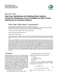
In Section 7 we show the following result. Theorem 1. Under the null hypothesis (2.3), the normalized maximum likelihood ratio test statistic has the asymptotic χ2 distribution with degree of freedom an : a rk λ∗n ∼ χ2an , where 2k/(2k+1) (2k + 1)2 4k + 2 π rk = , an = n1/(2k+1) . π 2k − 1 2k − 1 4k 2 sin( 2k )

Table 1 Constants rk (rk0 in Theorem 3) and degrees of freedom in Theorem 1

k rk an , n = 50 an , n = 200 an , n = 800 rk0

1 6.0000 28.2245 44.8036 71.1212 3.6923

2 3.3333 6.5381 8.6270 11.3834 2.5600

3 2.8000 3.8381 4.6787 5.7034 2.3351

4 2.5714 2.8800 3.3596 3.9190 2.2391

5 2.4444 2.4012 2.7237 3.0895 2.1858

It is clear from Theorem 1 that the classical Wilks type of results do not hold for infinite dimensional problems because rk 6= 2. However, an extended version holds: asymptotic null distributions are independent of nuisance parameters and nearly χ2 -distributed. Table 1 gives numerical values for constant rk and degrees of freedom an . Note that as the degree of smoothness k tends to ∞, rk → 2. Surprisingly, the maximum likelihood ratio test can not achieve the optimal rate for hypothesis testing (see Theorem P∞2 below). This is due to the fact the smoothing parameter ξˆ determined by j=1 j 2k θˆj2 = 1 is too restrictive. This is why we need generalized likelihood ratio tests which allow one the flexibility of choosing smoothing parameters. Theorem 2. There exists a θ ∈ Fk satisfying kθk = n−(k+d)/(2k+1) with d > 1/8 such that the power function of the maximum likelihood ratio test at the point θ is bounded by α, namely, lim sup Pθ {rk λ∗n > an + zα (2an )1/2 } ≤ α, where zα is the upper α quantile of the standard normal distribution.


9

Thus, the maximum likelihood ratio test λ∗n can detect alternatives with a rate no faster than n−(k+d)/(2k+1) . When k > 1/4, by taking d sufficiently close to 1/8, the rate n−(k+d)/(2k+1) is slower than the optimal rate n−2k/(4k+1) given in Ingster (1993). 2.3. Generalized likelihood ratio tests. As demonstrated in Section 2.2, maximum likelihood ratio tests are not optimal due to restrictive choice of smoothing parameters. Generalized likelihood tests remove this restrictive requirement and allow one to tune the smoothing parameter. For testing problem (2.3), we take the generalized likelihood ratio test as ∞ nX j 4k ξn2 (2.6) λn = 1− Yj2 , 2 j=1 (1 + j 2k ξn )2 with ξn = cn−4k/(4k+1) for some c > 0. This ameliorated procedure achieves the optimal rate of convergence for hypothesis testing, which is stated as follows. Theorem 3. rk0 = a0n

a

Under the null hypothesis (2.3), rk0 λn ∼ χ2a0n , where 2k + 1 48k 2 · , 2 2k − 1 24k + 14k + 1

(2k + 1)2 24k 2 c−1/(2k) π = · n2/(4k+1) . π 2k − 1 24k 2 + 14k + 1 4k 2 sin( 2k )

Furthermore, for any sequence cn → ∞, the power function of the generalized likelihood ratio test is asymptotically one: ( ) rk0 λn − a0n p inf Pθ > zα → 1. θ∈Fk : kθk≥cn n−2k/(4k+1) 2a0n 2.4. Adaptive minimaxity. The maximum likelihood ratio statistic (2.5) and the generalized likelihood statistic (2.6) depend critically on the value of k. Can we construct an adaptive version that achieves adaptively the optimal rates of convergence? The answer is affirmative and the construction is simple. Based on power considerations, Fan (1996) proposed the following adaptive version of the generalized likelihood ratio statistic (2.4): (2.7)

∗ TAN = max

1≤m≤n

m X

√ (nYi2 − 1)/ 2m.

i=1

He called the testing procedure as the adaptive Neyman test. Note that the adaptive Neyman test is simply the maximum of the normalized likelihood ratio statistic (2.4). It does not depend on the degree of smoothness. Following Fan (1996), we normalize the test statistic as p ∗ TAN = 2 log log nTAN − {2 log log n + 0.5 log log log n − 0.5 log(4π)}. Then, under the null hypothesis (2.3), we have P (TAN < x) → exp(− exp(−x)),

as n → ∞.

10


Thus, the critical region TAN > − log{− log(1 − α)} has asymptotic significance level α. The power of the adaptive Neyman test is given as follows. A similar version was presented in Fan and Huang (1998). Theorem 4. with rates

The adaptive Neyman test can detect adaptively the alternatives δn = n−2k/(4k+1) (log log n)k/(4k+1)

when the parameter space is Fk with unknown k. More precisely, for any sequence cn → ∞, the power function inf

θ∈Fk : kθk≥cn δn

Pθ [TAN > − log{− log(1 − α)}] → 1.

The rate given in Theorem 4 is adaptively optimal in the sense that no testing procedure can detect adaptively the alternative with a rate faster than δn , according to Spokoiny (1996). Hence, the generalized likelihood ratio test achieves this adaptive optimality. Remark 2.1. By choosing the parameter m = O(n2/(4k+1) ) when the parameter space is Fk , the Neyman test can also detect alternatives with the optimal rate O(n−2k/(4k+1) ). This follows from the proof of Theorem 4. By choosing m to maximize (2.7), we obtain an adaptive version of the Neyman test, which is independent of the degree of smoothness k. This test achieves the adaptive optimal rate because the maximum of the partial sum process in (2.7) grows very slowly. This is why we pay only a price of order (log log n) to achieve the adaptive minimax rate. 3. Generalized likelihood ratio tests in varying coefficient models. In this section we develop asymptotic theory on the generalized likelihood ratio statistics which are based on the local polynomial estimators and derive the optimal minimax rates of the corresponding tests under model (1.2). Wilks phenomenon is unveiled in this general setting. Suppose {(Yi , Xi , Ui )}ni=1 are a random sample from the varying-coefficient model (1.2). Namely, Y = A(U )τ X + ε,

ε ∼ N (0, σ 2 ),

with X = (X1 , · · · , Xp )τ , U = (U1 , · · · , Uq )τ , and A(U ) = (a1 (U ), · · · , ap (U ))τ . For simplicity, we consider only q = 1. Extensions to the multi-dimensional case are similar. Consider the simple null hypothesis testing problem: (3.1)

H0 : A = A0 ,

←→

H1 : A 6= A0 .

We use the local linear approach to construct a generalized likelihood ratio statistic.


11

For each given u0 , let β(u0 ) = (A(u0 )τ , hA0 (u0 )τ )τ . Let β = (A∗ , hB τ )τ . where A∗ and B are vectors of p-dimensions. Then, the local log-likelihood at the given point u0 is given by n √ 1 X l(β) = −n log( 2πσ) − 2 (Yi − β τ Zi )2 Kh (Ui − u0 ), 2σ i=1

where Zi = Zi (u0 ) = (Xτi , (Ui − u0 )/hXτi )τ and Kh (·) = K(·/h)/h with K being a symmetric probability density function and h a bandwidth. Then, the local ˆ 0 ), is defined as argmax l(β). The maximum likelihood estimator, denoted by β(u ˆ 0 ). Using this nonparametric corresponding estimator of A(u0 ) is denoted by A(u estimator, the likelihood under model (1.2) is √ −n log( 2πσ) − RSS1 /(2σ 2 ), Pn ˆ k )τ Xk )2 . Maximizing over the parameter σ 2 leads where RSS1 = k=1 (Yk − A(U to the generalized likelihood under model (1.2): `n (H1 ) = −(n/2) log(2π/n) − (n/2) log(RSS1 ) − n/2. Similarly, the maximum likelihood under H0 can be expressed as `n (H0 ) = −(n/2) log(2π/n) − (n/2) log(RSS0 ) − n/2, Pn τ 2 where RSS0 = k=1 (Yk − A0 (Uk ) Xk ) . Now, the generalized likelihood ratio statistic is n RSS0 n RSS0 − RSS1 (3.2) λn (A0 ) = [`n (H1 ) − `n (H0 )] = log ≈ , 2 RSS1 2 RSS1 In general, the above approach can often be extended to the composite null hypothesis testing problem: (3.3)

H0 : A ∈ A 0 ,

←→

H1 : A 6∈ A0

where A0 is a set of functions. As before, we can use the local linear estimator to construct the log-likelihood `n (H1 ) for H1 . Assume that we can use MLE or some local linear estimators to build the log-likelihood `n (H0 ). Let A00 denote the true value of the parameter A. Then the generalized likelihood ratio λn (A0 ) for the testing problem (3.3) can be decomposed as (3.4)

λn (A0 ) = λn (A00 ) − λ∗n (A00 ),

where λn (A00 ) = `n (H1 ) − `n (H00 ) is the generalized likelihood ratio for the hypothesis testing problem H00 : A = A00 ,

←→

H1 : A 6= A00

and λ∗n (A00 ) = `n (H0 ) − `n (H00 ) is the likelihood ratio for another hypothesis testing problem H00 : A = A00 ,

←→

H10 : A ∈ A0 .

12


The above two hypothesis problems are fabricated because A00 is unknown. Therefore the generalized likelihood ratio for the composite null hypothesis can be decomposed into two generalized likelihood ratios for two fabricated simple null hypothesis problems. As in the proof of Theorem 5, generally the asymptotic representation of the generalized likelihood ratio for the composite null hypothesis can be derived from those of the above fabricated simple null hypothesis problems. Then, the asymptotic theory for composite null hypothesis can be easily obtained (see the proofs of Theorems 6 and 9, Remark 3.4 and the results in Fan and Zhang (1999)). Thus, we focus first on the simple null hypothesis testing problem (3.2). In order to include the above fabricated testing problems, we assume that A0 is unknown. We should point out that for model (1.2), when A0 is known, the testing problem (3.2) is equivalent to the problem H0 : A = 0 by a simple transform. 3.1. Asymptotic null distribution. To derive the asymptotic distribution of λn (A0 ) under H0 , we need the following conditions. Condition (A) (A1) The marginal density f (u) of U is Lipschitz continuous and bounded away from 0. U has a bounded support Ω. (A2) A(u) has the continuous second derivative. 3 (A3) The function K(t) is symmetric R and bounded. Further, the functions t K(t) and t3 K 0 (t) are bounded and t4 K(t)dt < ∞.

(A4) E|ε|4 < ∞. (A5) X is bounded. The p × p matrix E(XXτ |U = u) is invertible for each u ∈ Ω. −1 (E(XXτ |U = u)) and E(XXτ σ 2 (X, U )|U = u) are both Lipschitz continuous. These conditions are imposed to facilitate the technical arguments. They are not weakest possible. In particular, (A5) in Condition (A) can be relaxed by using the method in Lemma 7.4 in Zhang and Gijbels (1999). For example, we can replace the assumption that X is bounded in (A5) by the assumption that E exp(c0 ||X||) < ∞ for some positive constant c0 . The following results continue to hold. Note that in the above conditions, the normality of ε is not needed. Define Z Z Γ(u) = E[XXτ |U = u]f (u), w0 = t2 (s + t)2 K(t)K(s + t)dtds. Let εi = Yi − A0 (U )τ Xi . Set n

1 X Rn10 = √ εi A000 (Ui )τ Xi n i=1

Z

t2 K(t)dt(1 + O(h) + O(n−1/2 )),

n

Rn20 =

1 1 X √ εi Xτi Γ(Ui )−1 A000 (Ui )τ E(Xi |Ui )w0 , 2 n i=1

Rn30 =

1 EA000 (U )τ XXτ A000 (U )w0 (1 + O(n−1/2 )), 8

13


Z 1 p|Ω| (K(0) − K 2 (t)dt), h 2 Z 2p|Ω| 1 σn2 = (K(t) − K ∗ K(t))2 dt, h 2

µn =

d1n = σ −2 {nh4 Rn30 − n1/2 h2 (Rn10 − Rn20 )} = Op (nh4 + n1/2 h2 ), where K ∗ K denotes the convolution of K. Note that both Rn10 and Rn20 are asymptotically normal and hence are stochastically bounded. We now describe our generalized Wilks type of theorem as follows: Theorem 5. nh3/2 → ∞,

Suppose Condition (A) holds. Then, under H0 , as h → 0, L

σn−1 (λn (A0 ) − µn + d1n ) −→ N (0, 1). a

Furthermore, if A0 is linear or nh9/2 → 0, then as nh3/2 → ∞, rK λn (A0 ) ∼ χ2rK µn , where R K(0) − 12 K 2 (t)dt rK = R . (K(t) − 12 K ∗ K(t))2 dt Remark 3.1. As pointed out before, for model (1.2), when A0 is known, the testing problem (3.2) is equivalent to the problem H0 : A = 0 ←→ H1 : A 6= 0 by a simple transform. Hence, the condition in the second part of the theorem always holds and so does the Wilks phenomenon. Further, when nh5 → 0, the mean and variance of λn is free of nuisance parameters up to the first order because d1n = o(µn ). In this relaxed sense, even if A0 is unknown, the Wilks phenomenon is valid when the condition nh9/2 → 0 is relaxed as nh5 → 0. Remark 3.2. The degree of freedom in the asymptotic distribution depends on p|Ω|/h. This can intuitively be understood as follows. If one partitions the support of U into intervals of length h and uses piecewise constant functions to model the functions in A, then we have total number of parameters p|Ω|/h under model (1.2). In this view, local linear fits can also be regarded as sieve approximation to nonparametric functions with effective number of parameters rK µn . Remark 3.3. If local polynomial estimators of degree v instead of the local linear estimators are used to construct the above generalized likelihood ratio, then the result holds when K is replaced by its equivalent kernel induced by the local polynomial fitting (Fan and Gijbels, 1996). In this case, the second part of Theorem 5 is replaced by the condition that either A0 is a polynomial of degree v or nh(4v+5)/2 → 0. Remark 3.4. Suppose Condition (A) holds and the second term in (3.4) is op (h−1/2 ) (for example, in testing a parametric model, under some regularity conditions this term equals Op (1)). Then it follows directly from Theorem 5 that under the null hypothesis (3.3) the result in Theorem 5 continues to hold.

14


We now consider the more challenging and more interesting case where null hypotheses depend on many nuisance functions. Nevertheless, we will show that asymptotic null distributions are independent of the nuisance functions. Write ! ! (1) (1) A10 (u) A1 (u) Xk Zk A0 (u) = , A(u) = , Xk = , Zk = (2) (2) A20 (u) A2 (u) X Z k

where A10 (u), A1 (u), problem (3.5)

(1) Xk

and

(1) Zk

H0u : A1 = A10

k

are p1 (< p) dimensional. Consider the testing ←→

H1u : A1 6= A10

with A2 (·) completely unknown. For the same purpose mentioned above, (3.5) is allowed to be a fictitious testing problem in which the function A10 is unknown. Following the same derivations, the logarithm of the generalized likelihood ratio statistic is given by λnu (A10 ) = λn (A0 ) − λn2 (A20 |A10 ) with λn (A0 ) the full likelihood ratio defined in (3.2) and λn2 (A20 |A10 ) =

n RSS0 log 2 RSS2

where RSS2 =

n X

k=1

(1) e2 (Uk )τ X(2) )2 . (Yk − A10 (Uk )τ Xk − A k

e2 (Uk )τ is the local linear estimator at Uk when A10 is given. Here A Recall that Γ(u) = E[XXτ |U = u]f (u). Write Γ11 Γ12 Γ= , and Γ11,2 = Γ11 − Γ12 Γ−1 22 Γ21 , Γ21 Γ22 where Γ11 , Γ12 , Γ21 , Γ22 are p1 × p1 , p1 × p2 , p2 × p1 and p2 × p2 matrices and p2 = p − p1 . Define µnu and σnu the same as µn and σn except replacing p by p1 . Similarly, define d1nu by replacing X and Γ respectively by X(1) − Γ12 Γ22 X(2) and Γ11,2 in the definition of d1n . Theorem 6. Suppose Condition (A) holds. Then, under H0u in (3.5), as nh3/2 → ∞ and h → 0, we have L

σn−1 (λnu (A0 ) − µnu + d1nu ) −→ N (0, 1). In addition, if A0 is linear or nh9/2 → 0, then a

rK λnu (A0 ) ∼ χ2rK µnu . Theorem 6 provides convincing evidence that the Wilks type of phenomenon holds for generalized likelihood ratio tests with composite hypotheses.


15

3.2. Power approximations and minimax rates. We now consider the power of generalized likelihood ratio tests based on local linear fits. For simplicity of our discussion, we focus only on the simple null hypothesis (3.1). As noted in Remark 3.1, one can assume without loss of generality that A0 = 0. But, we don’t take this option because we want to examine the impact of biases on generalized likelihood ratio tests. This has implications to the case of composite hypothesis (3.5) because the biases inherited in that problem are genuine. When A0 is linear, the bias term in Theorem 5 will be zero. When A0 is not linear, we will assume that hn = o(n−1/5 ) so that the second term in the definition of d1n is of smaller order than σn . As to be seen in Theorem 8, the optimal choice of h for the testing problem (3.1) is h = O(n−2/9 ), which satisfies the condition h = o(n−1/5 ). Under these assumptions, if nh3/2 → ∞, by Theorem 5, an approximate level α test based on the generalized likelihood ratio statistic is φ ≡ φh = I{λn (A0 ) − µn + vˆn ≥ zα σn }, 2

where with σ ˆ = RSS1 /n, vˆn =

1 4 −2 nh σ ˆ EA000 (U )τ XXτ A000 (U ) 8

Z Z

t2 (s + t)2 K(t)K(s + t)dtds.

The power of the test under the contiguous alternative of form H1n : A(u) = A0 (u) + Gn (u), can be approximated by using the following theorem, where Gn (u) = (g1n (u), · · · , gpn (u))τ ) is a vector-valued function. Theorem 7.

Suppose that Condition (A) hold and that A0 is linear or nh5 → 0.

If nhEGτn (U )XXτ Gn (U ) → C(G)

and

E(Gτn (U )XXτ Gn (U )2 )2 = O((nh)−3/2 ),

for some constant C(G), then under H1n L

(λn (A0 ) − µn + vˆn + v2n − d2n )/σn∗ −→ N (0, 1), where n EGτn (U )XXτ Gn (U ), 2 p σn∗ = σn2 + nσ −2 EGτn (U )XXτ Gn (U ), Z Z nh4 τ 00 00 τ v2n = EGn (U ) XX Gn (U ) t2 (s + t)2 K(t)K(s + t)dtds. 8σ 2

d2n =

Theorem 7 can be extended readily to generalized likelihood ratio tests based on local polynomial estimators of degree v and to the case with nuisance parameter functions. It allows functions Gn of forms not only gn (u) = (nh)−1/2 g(u), but −1/5 also gn (u) = a−2 . The former function has a second n g(an u) with an = (nh) derivative tending to zero, which is restrictive in nonparametric applications. The latter function has also a bounded second derivative, which does not always tend to

16


zero, when g is twice differentiable. This is still not the hardest alternative function to be tested. A harder alternative can be constructed as follows. Let {uj } be a grid of points with distance a−1 n apart and g be a twice differentiable function P with support [0, 1]. Then, Theorem 7 also allows functions of form gn (u) = a−2 n j g(an (u − uj )) with an = (nh)−1/4 . We now turn to studying the optimal property of the generalized likelihood ratio test. We first consider the class of functions Gn , satisfying the following regularity conditions: var(Gτn (U )XXτ Gn (U )) ≤ M (EGτn (U )XXτ Gn (U ))2 , (3.6)

nEGτn (U )τ XXτ Gn (U ) > Mn → ∞, EG00n (U )τ XXτ G00n (U ) ≤ M,

for some constants M > 0 and Mn → ∞. For a given ρ > 0, let Gn (ρ) = {Gn ∈ Gn : EGτn (U )XXτ Gn (U ) ≥ ρ2 }. Then the maximum of the probabilities of type II errors is given by β(α, ρ) =

sup

β(α, Gn ),

Gn ∈Gn (ρ)

where β(α, Gn ) = P (φ = 0|A = A0 + Gn ) is the probability of type II error at the alternative A = A0 + Gn . The minimax rate of φ is defined as the smallest ρn such that (i) for every ρ > ρn , α > 0, and for any β > 0, there exists a constant c such that β(α, cρ) ≤ β + o(1); (ii) for any sequence ρ∗n = o(ρn ), there exist α > 0, β > 0 such that for any c > 0, P (φ = 1|A = A0 ) = α + o(1) and lim inf n β(α, cρ∗n ) > β. It measures how close the alternatives that can be detected by the generalized likelihood ratio test φh . The rate depends on the bandwidth h. To stress its dependence, we write it as ρn (h). Theorem 8. Under Condition (A), the generalized likelihood can detect alternatives with rate ρn (h) = n−4/9 when h = c∗ n−2/9 for some constant c∗ . Remark 3.5. When p = 1 and X ≡ 1, the varying-coefficient model becomes an ordinary nonparametric regression model. In this case, Lepski and Spokoiny (1995) proved the optimal rate for testing H0 is n−4/9 . Thus the generalized likelihood ratio test is optimal in the sense that it achieves the optimal rate of convergence. Similarly, we can show the generalized likelihood ratio test, constructed by using local polynomial of order v, can detect alternatives with rate n−2(v+1)/(4v+5) , uniformly in the class of functions satisfying E[G(v+1) (U )τ X]2 < M, n for some M < ∞. The corresponding optimal bandwidth is c∗ n−2/(4v+5) for some constant c∗ .

17


Remark 3.6. In the proof of Theorem 8, we in fact show that the bandwidth h = c∗ n−2/9 is optimal, optimizing the rate of ρn (h), subject to the following constrains: (a) h → 0 and nh3/2 → ∞, if A0 is linear. (b) nh → ∞ and nh5 → 0, if A0 is non-linear with continuous second derivatives. 4. Model diagnostics. In this section, we demonstrate how the generalized likelihood ratio tests can be applied to check the goodness-of-fit for a family of parametric models. This kind of problems occur very often in practice. Our results apply readily to this kind of problems. We also note that the Wilks phenomenon continue to hold under general heteroscedastic regression models. 4.1. Testing linearity. Consider the nonparametric regression model (1.3) and the testing problem ←→

H0 : m(x) = α0 + α1 x

H1 : m(x) 6= α0 + α1 x,

where α0 and α1 are unknown parameters. Following the same derivations as in Section 3, generalized likelihood ratio tests based on local linear fits are given by RSS0 n log , 2 RSS1 Pn Pn where RSS0 = ˆ0 − α ˆ 1 Xi )2 and RSS1 = ˆ h (Xi ))2 . By i=1 (Yi − α i=1 (Yi − m using Remark 3.4, one can easily see that Wilks type of results hold under the null hypothesis: λn = [`n (H1 ) − `n (H0 )] =

a

rK λn ∼ χ2rK cK |Ω|/h ,

(4.1)

where Ω denotes the support of X, and cK = K(0) − 2−1 kKk22 . Note that when K(0) = max K(x), we have K(0) ≥ kKk22 , cK ≥ 2−1 K(0) and x whence rK > 0. To help one determine the degree of freedom in (4.1), the values of rK and cK are tabulated in Table 2 for a few commonly-used kernels. Among them, the Epanechnikov kernel has the closest rK to 2. Table 2 Values of rK and cK in (4.1)

Kernel rK cK

Uniform 1.2000 0.2500

Epanechnikov 2.1153 0.4500

Biweight 2.3061 0.5804

Triweight 2.3797 0.6858

Gaussian 2.5375 0.7737

Two inter-relationships concerning the degrees of freedom will be exposed. If we define a “smoothing matrix” H based on local linear estimates just as a projection matrix P in the linear regression model, then under H0 , RSS0 −RSS1 = ετ (H τ +H −

18


H τ H −P )ε. Denoting the bracket matrix as A, we have tr(A) ≈ 2cK |Ω|/h following the proof of Theorem 5. Thus, tr(A) is approximately the degree of freedom only when rK ≈ 2. The second one is to note that K(0) ≥ K ∗ K(0) = kKk22 implies approximately tr(H τ H) ≤ tr(H) ≤ 2tr(H) − tr(H τ H), a property holding exactly for H based on smoothing splines in fixed designs [Hastie and Tibshirani (1990), section 3.5]. Remark 4.1. When one wishes to test parametric families other than the linear model such as H0 : m(x) = m(x, θ), then one can apply generalized likelihood ratio ˆ where m(Xi , θ) ˆ is a fitted value under the null tests to the residuals {Yi − m(Xi , θ)}, hypothesis. The Wilks type of result (4.1) continues to hold. Remark 4.2. For more general regression model (1.3), where we assume only E(ε|X = x) = 0 and E(ε2 |X = x) = σ 2 (x), one can use the weighted residual sum of squares: RSS0 =

n X

2

(Yi − α ˆ0 − α ˆ 1 Xi ) w(Xi ),

RSS1 =

i=1

n X

(Yi − m ˆ h (Xi ))2 w(Xi ).

i=1

If the weight function w(·) is continuous with a compact support contained in {x : f (x) > 0}, then we can show that under H0 , a generalized version of (4.1): a

0 rK λn ∼ χ2a0n ,

where 0 rK = rK [Eσ 2 (X)w(X)]

a0n = rK cK h−1

Z

Z

σ 2 (x)w(x)dx

Z

−1 σ 4 (x)w2 (x)dx ,

2 Z −1 σ 2 (x)w(x)dx σ 4 (x)w2 (x)dx .

When σ 2 (x) = v(x)σ 2 for a known function v(x), the generalized likelihood ratio test corresponds to using w(x) = v(x)−1 . In this case, the Wilks type of result (4.1) continues to hold. 4.2. Testing homogeneity. Consider the varying-coefficient model defined in Section 3. A natural question arises in practice is if these coefficient functions are really varying. This amounts to testing the following problem: H0 : a1 (U ) = θ1 , · · · , ap (U ) = θp . If the error distribution is homogeneous normal, then theP generalized likelihood test n based on local linear fits is given by (3.2) with RSS0 = i=1 (Yi − θˆτ Xi )2 where θˆ is the least-square estimate under the null hypothesis. To examine the property of the generalized likelihood ratio statistic (3.2) under the general heteroscedastic model, we now only assume that E(ε|X = x, U = u) = 0,

E(ε2 |X = x, U = u) = σ 2 (x, u),

19


with a continuous function σ 2 (x, u). Strictly speaking, the statistic (3.2) is no longer a generalized likelihood ratio test under this heteroscedastic model. The generalized likelihood ratio test in this heteroscedastic case should involve weighted residual sum of squares when σ 2 (x, u) = σ 2 v(x, u) for a given v. See Remark 4.2. Let Γ∗ (u) = E[XXτ σ 2 (X, U )|U = u]f (u). Then, we have the following result. Theorem 9.

Assume Condition (A). Then under H0 , as h → 0, nh3/2 → ∞, a

00 rK λn ∼ χ2a00n ,

where 00 rK = rK [Eσ 2 (X, U )]

Z

tr(Γ∗ (u)Γ(u)−1 )du

Z

Ω

a00n = rK cK h−1

Z

tr(Γ∗ (u)Γ(u)−1 )du

Ω

tr(Γ∗ (u)Γ(u)−1 )2 du

−1

,

Ω

2 Z

tr(Γ∗ (u)Γ(u)−1 )2 du

−1

.

Ω

It is clear that when σ 2 (x, u) = σ 2 , Theorem 9 reduces to Theorem 5 and (3.2) is a generalized likelihood statistic. Hence the Wilks type of result continues to hold for testing homogeneity. It can also be shown that the Wilks phenomenon is still valid for the generalized likelihood ratio in the heteroscedastic model with σ 2 (x, u) = σ 2 v(x, u), bearing in mind that generalized likelihood ratio statistics are now based on weighted residual sum of squares. 5. Extensions. The Wilks type of results hold not only for the various problems that we have studied. They should be valid for nearly all regular nonparametric testing problems. In this section, we mention various possible extensions to indicate their versatility. 5.1. Generalized varying coefficient models. The inferences on generalized varying coefficient models have been empirically studied by Hastie and Tibshirani (1993) and Cai, Fan and Li (2000). The results in the previous sections can be directly extended to this setting. Consider a generalized varying-coefficient model with the following log-likelihood function l{g −1 (η(x, u)), y} = g0 (g −1 (η(x, u)))y − b(g0 (g −1 (η(x, u)))) where η(x, u) = g(m(x, u)) = A(u)τ x, g is called a link function and g0 = b0 is the canonical link. Poisson regression and logistic regression are two prototype examples. Define l(g −1 (s), y) = g0 (g −1 (s))y − b(g0 (g −1 (s))),

20


q1 (s, y) =

g 0 (s) ∂l{g −1 (s), y} = 00 (y − b0 (s)), ∂s g (s)

∂ 2 l{g −1 (s), y} = (g000 /g 0 − g00 g 00 /(g 02 ))(y − g −1 (s)) − g00 /(g 0 )2 , ∂s2 ∂ 3 l{g −1 (s), y} q3 (s, y) = ∂s3 000 = (g0 /g 0 − g000 g 00 /g 02 − (g000 g 00 + g 000 g00 )/g 02 + 2g00 g 002 /g 03 )(y − g −1 (s)) − 2g000 /g 02 − g00 g 00 /g 03 . q2 (s, y) =

In particular, when g = g0 is the canonical link, we have q2 (s, y) = −b00 (s),

q3 (s, y) = −b000 (s).

As in Section 3, we can define a local linear estimator Aˆ for A. Lemma 7.5 yields the following asymptotic representation for Aˆ : ˆ 0 ) − A(u0 ) = r2 Γ(u e 0 )−1 A(u n

n X

εi Xi K((Ui − u0 )/h)(1 + op (1)) + Hn (u0 )(1 + op (1)),

i=1

where e 0 ) = −E[q2 (Aτ (u0 )X, Y )XXτ |U = u0 ]f (u0 ), Γ(u Hn (u0 ) =

n X

e 0 )−1 rn2 Γ(u

εi = q1 (A(Ui )τ Xi , Yi ),

[q1 (β(u0 )τ Zi , Yi ) − q1 (A(Ui )τ Xi , Yi )]Xi K((Ui − u0 )/h).

i=1

The generalized likelihood ratio for testing the null hypothesis H0 : A = A0 is defined as λng (A0 ) = −

n X

ˆ i )T Xi ), Yi } − l{g −1 (Ai (Ui )τ Xi ), Yi }]. [l{g −1 (A(U

i=1

Denote qn∗ = qn∗ (U, X, Y ) =

|q2 (β(u0 )τ Z(u0 ) + ατ Z(u0 ), Y )|K(

sup u0 ,||α||≤c1 rn

U − uo ) h

√ where rn = 1/ nh. For j = 1, 2, 3 and c1 > 0, define Φnj = Φnj (U, X, Y ) =

sup

|q2 (β(u0 )τ Z(u0 )+ατ Z(u0 ), Y )||

uo ,||α||≤c1 rn

The following technical conditions are needed: Condition (B) (B1) E|q1 (A(U )τ X, Y )|4 < ∞. (B2) E[q2 (A(U )τ X)XXτ |U = u] is Lipschitz continuous.

U − u0 j−1 U − u0 | K( ). h h

21


(B3) The function q2 (s, y) < 0 for s ∈ R and y in the range of the response variable. For some function q∗ (y), si ∈ C, i = 1, 2, |q2 (s1 , y) − q2 (s2 , y)| ≤ q∗ (y)|s1 − s2 |. Further, for some constant ξ > 2, E{Φnj (U, X, Y ) ||XXτ ||}ξ = O(1), 2

Eq∗ (Y )||X||3 < ∞,

Eqn∗ (U, X, Y )||X|| = O(1), sup

j = 1, 2, 3,

Eq22 (β(u0 )τ Z(u0 ) + ατ Z(u0 ), Y )K 2 ((U − u0 )/h)/h||XX τ ||2 = O(1), j = 1, 2, 3.

u0 ,||α||≤c1 rn

Set n

1 X Rn10g = √ εi A000 (Ui )τ Xi n i=1

Z

t2 K(t)dt(1 + O(h) + O(n−1/2 )),

n

1 1 X e i )−1 A000 (Ui )τ E(q2 (Aτ0 (U )τ X)X|Ui )w0 , εi Xτi Γ(U Rn20g = − √ 2 n i=1 1 Rn30g = − EA000 (U )τ q2 (A0 (U )τ X, Y )XXτ A000 (U )w0 (1 + O(n−1/2 )), 8 RR 2 where w0 = t (s + t)2 K(t)K(s + t)dtds. Note that both Rn10g and Rn20g are asymptotic normal and hence stochastically bounded. Let d1ng = nh4 Rn30g − n1/2 h2 (Rn10g − Rn20g ). Then, d1ng = nh4 Rn30g (1 + op (1)) if n1/2 h2 → ∞. The following theorem shows that the Wilks type of results continue to hold for generalized varying coefficient models. Theorem 10. Under Conditions (A1) – (A3) and (B1) – (B3), as h → 0, nh3/2 → ∞ and n(ξ−1)/ξ h ≥ c0 (log n)δ for some δ > (ξ − 1)/(ξ − 2), we have the following asymptotic null distribution: L

σn−1 (λng (A0 ) − µn + d1ng ) −→ N (0, 1). a

Furthermore, if A is linear or nh9/2 → 0, then as nh → ∞, rK λng (A0 ) ∼ χ2rK µn , where µn and rK are given in Theorem 5. Extensions of the other theorems and the remarks in Section 3 are similar. In particular the optimal minimax rate and the optimal bandwidth are the same as those in Section 3. The generalized likelihood ratio tests can be employed to check the inhomogeneity of the coefficient functions and significance of variables in the generalized varying-coefficient models. The related theorems in Section 4 hold true after some mild modifications. The details are omitted. 5.2. Empirical likelihoods. As pointed out in the introduction, neither Owen’s empirical likelihood nor its extension, random sieve likelihood [Shen, Shi and Wong (1999)] can be directly used to make inferences on a nonparametric regression function. However, the idea of sieve empirical likelihood [Zhang and Gijbels (1999)] can be effective in this situation. In a forthcoming manuscript, Fan and Zhang (1999) have developed the corresponding theory. The advantages of sieve empirical likelihood ratios include that no parametric models are needed for stochastic errors

22


and that it adapts automatically for inhomogeneous stochastic errors. The main disadvantage is that it requires intensive computation. 6. Discussion. 6.1. Other tests. There are many nonparametric tests designed for certain specific problems. Most of them are in univariate nonparametric regression setting. See Section 1.5 for an overview of the literature. While they can be powerful for their problems where the tests were designed, extensions of these tests to multivariate setting can pose some challenges. Further, these tests are usually not distribution free, when null hypotheses involve nuisance functions. This would hamper their applicability. Nonparametric maximum likelihood ratio tests are a natural alternative. Usually, they do usually exist. If they do, they are hard to find. Further, as shown in Section 2.2, they are not optimal. For this reason, they can not be a generic and powerful method. 6.2. Conclusions. The generalized likelihood method is widely applicable. It applies not only to univariate setting, but also to multivariate nonparametric problems. It is ready to use because of the Wilks phenomenon. It is powerful since it achieves optimal rates of convergence. It can also be adaptively minimax when tuning parameters are properly tuned (Section 2.4). The tuning method for local polynomial based generalized likelihood ratio test can be surprisingly simple. Motivated by the adaptive Neyman test constructed in Fan (1996), when the null hypothesis is linear, an adaptive construction of the generalized likelihood would naturally be (6.1)

∗ TASL =

max

h∈[n−a ,n−b ]

rλn (h) − d(h) p , 2d(h)

for some a, b > 0,

where r is the normalizing constant, λn (h) is the generalized likelihood ratio test and d(h) is the degrees of freedom. Therefore, the generalized likelihood is a very useful principle for all nonparametric hypothesis testing problems. While we have observed the Wilks phenomenon and demonstrated it for a few useful cases, it is impossible for us to verify the phenomenon for all nonparametric hypothesis testing problems. The Wilks phenomenon needs to be checked for other problems that have not been covered in this paper. More work is needed in this direction. 7. Proofs. Proof of Lemma 2.1. For each given ξn,c = cn−2k/(2k+1) (c > 0), under the null hypothesis (2.3), by using the mean-variance decomposition, we have X X j 4k j 2k −1 1/2 −1 (7.1) F (ξn,c ) = n + Op n { } . (1 + j 2k ξn,c )2 (1 + j 2k ξn,c )4

23


Note that gn (x) =

x2k (1+x2k ξn,c )2

−1/(2k)

is increasing for 0 ≤ x ≤ ξn,c

and decreasing for

−1/(2k) ξn,c .

x≥ By using the unimodality of gn and approximating discrete sums by their corresponding integrals, one can show that Z ∞ X y 2k j 2k −(2k+1)/(2k) (7.2)n−1 = c dy + O(n−1/(2k+1) ). (1 + j 2k ξn,c )2 (1 + y 2k )2 0 Using the same arguments as those obtaining (7.2), we have X n−1 { j 4k (1 + j 2k ξn,c )−4 }1/2 = O[n−1/{2(2k+1)} ]. This together with (7.1) and (7.2) yield F (ξn,c ) = (c0 /c)(2k+1)/(2k) + Op (n−1/{2(2k+1)} ), R ∞ 2k where c0 = ( 0 y (1 + y 2k )−2 dy)2k/(2k+1) . For any ε > 0, since the function F (x) is strictly decreasing, (7.3)

ˆ n,c )| > ε) = P (F (ξ) ˆ < F (ξn,c +ε ))+P (F (ξ) ˆ > F (ξn,c −ε )) = o(1), P (|n2k/(2k+1) (ξ−ξ 0 0 0 which implies ξˆ − ξn,c0 = op (n−2k/(2k+1) ).

Proof of Theorem 1. F (j; ξ) =

Define the j-th coefficients in F (ξ) and λ∗n as j 2k , (1 + j 2k ξ)2

λ(j; ξ) =

1 + 2j 2k ξ . (1 + j 2k ξ)2

Then (7.4)

F 0 (j; ξ) = −

2j 4k , (1 + j 2k ξ)3

λ0 (j; ξ) = −

2j 4k ξ = ξF 0 (j; ξ). (1 + j 2k ξ)3

Let c0 be defined the same as in Lemma 2.1. For any ηn,j between ξˆ and ξn,c0 , it can easily be shown that 0 F (j; ηn,j ) − F 0 (j; ξn,c0 ) = op (1) (7.5) sup F 0 (j; ξn,c ) j≥1 0

and that for any ζn,j between ξˆ and ξn,c0 , 0 λ (j; ζn,j ) − λ0 (j; ξn,c0 ) = op (1). sup (7.6) λ0 (j; ξn,c ) j≥1 0

1 2

1+2j 2k ξ 2 j=1 (1+j 2k ξ)2 εj .

P∞

Let λn (ξ) = By using Taylor’s expansion together with (7.4), (7.5) and (7.6), under the null hypothesis (2.3), ∞ i 1 Xh λ∗n = λ(j; ξn,c0 ) + (ξˆ − ξn,c0 )λ0 (j; ζn,j ) ε2j 2 j=1 P∞ 0 1 2 j=1 λ (j; ξn,c0 )εj 2 ˆ (1 + op (1)) = λn (ξn,c0 ) + [F (ξ) − F (ξn,c0 )] 1 P∞ 2 0 j=1 F (j; ξn,c0 )εj n

24


n = λn (ξn,c0 ) + [1 − F (ξn,c0 )] ξn,c0 + op (n1/(2(2k+1)) ) 2 ∞ X 1 1 1 = ε2 + c0 n1/(2k+1) + op (n1/(2(2k+1)) ). 2 j=1 (1 + j 2k ξn,c0 ) j 2

(7.7)

Define λn,1 = we have

1 2

P∞

j=1 {1+j

2k

ξn,c0 }−1 ε2j in (7.7) and Vn =

1 2

Pn

j=1 {1+j

2k

ξn,c0 }−1 ε2j ,

n X max1≤j≤n {1 + j 2k ξn,c0 }−1 1/(4k) qP ≤ { (1 + j 2k ξn,c0 )−2 }−1/2 = O(ξn,c ) → 0, 0 n 2k −2 {1 + j ξ } j=1 n,c 0 j=1 L which implies that V√n −E(Vn ) −→ N (0, 1) by Lemma 2.1 of Huber (1973). Note that var(Vn ) Z Z 1 ∞ dx 1 ∞ dx −2 var(λn,1 − Vn ) ≤ ≤ = O(ξn,c n−(4k−1) ). 0 2k 2 4k 2 2 n (1 + x ξn,c0 ) 2 n x ξn,c 0

Hence var(λn,1 − Vn ) −2 −1/(2k) = O(ξn,c n−(4k−1) /ξn,c ) → 0. 0 0 var(λn,1 ) This implies that λn,1 − E(λn,1 ) L p −→ N (0, 1) var(λn,1 ) [by Theorem 3.2.15 of Randles and Wolfe (1979)], where Z ∞ Z ∞ dy dy −1/(2k) −1 −1/(2k) +O(1), var(λ ) = 2 ξ +O(1). E(λn,1 ) = 2−1 ξn,c n,1 n,c0 0 2k (1 + y ) (1 + y 2k )2 0 0 This together with (7.7) yield −1/(2k) 1/(2k+1) R ∞ 1+2y 2k dy L λ∗n − 2−1 c0 n 0 (1+y 2k )2 q −→ N (0, 1). −1/(2k) 1/(2k+1) R ∞ dy 2−1 c0 n 0 (1+y 2k )2 a

Namely, rk λ∗n ∼ χ2an , where Z ∞ −1 Z ∞ 1 + 2y 2k 1 rk = 2 dy dy , (1 + y 2k )2 (1 + y 2k )2 0 0 Z ∞ 1 + 2y 2k −1/(2k) −1 an = 2 rk c0 dy n1/(2k+1) . (1 + y 2k )2 0 Finally, by using Z Z 0

∞

0 ∞

dy 1 = π π, (1 + y 2k ) 2k sin( 2k )

Z 0

dy (2k − 1)(4k − 1) = π, π (1 + y 2k )3 16k 3 sin( 2k )

∞

dy (2k − 1) = 2 π π, (1 + y 2k )2 4k sin( 2k ) Z ∞ dy (2k − 1)(4k − 1)(6k − 1) = π, π 2k )4 (1 + y 96k 4 sin( 2k ) 0


25

we obtain 4k + 2 rk = , 2k − 1

2k/(2k+1) (2k + 1)2 π an = n1/(2k+1) . π 2k − 1 4k 2 sin( 2k )

Proof of Theorem 2. Take jn−k = n−(k+d)/(2k+1) . Let θ be a vector whose jn -th position is jn−k and the rest are zero. Then, θ ∈ Fk and kθk = n−(k+d)/(2k+1) . For ξn,c = cn−2k/(2k+1) , we have jn2k ξn,c = cn2d/(2k+1) . Under this specific alternative, by using model (2.2), we have for d > 1/8 jn2k (2j −k n−1/2 εjn +jn−2k ) = F (ξn,c |H0 )+op (n−1/{2(2k+1)} ), (1 + jn2k ξn,c )2 n P∞ j 2k where F (ξn,c |H0 ) = n−1 j=1 (1+j 2k ε2 . By the arguments as those in the ξn,c )2 j proof of Lemma 2.1, one can see that F (ξn,c ) = F (ξn,c |H0 )+

ξˆ = ξn,c0 (1 + op (1)), ˆ = 1. where ξˆ solves F (ξ) Next, consider the likelihood ratio statistic λ∗n under the alternative hypothesis. Let ! 1X j 4k ξˆ2 λn,0 = 1− ε2j . ˆ2 2 j (1 + j 2k ξ) Then for d > 1/8, λ∗n

n = λn,0 + 2

1−

jn4k ξˆ2 ˆ2 (1 + jn2k ξ)

!

(2jn−k n−1/2 εjn + jn−2k ) = λn,0 + op (n1/{2(2k+1)} ). a

By similar proof of Theorem 1, rk λn,0 ∼ χ2an , which entails that Pθ {rk λ∗n > an + zα (2an )1/2 } = α + o(1).

Proof of Theorem 3. This first part of result follows directly from the central limit theory using similar arguments to those in the proof of Theorem 1 for λn,1 . We now establish the power of the test. Under the alternative hypothesis, ∞ X j 4k ξn2 0 0 0 Eθ (rk λn ) = an + O(1) + rk 1− nθj2 /2 2k ξ )2 (1 + j n j=1 and varθ (rk0 λn ) = 2a0n + b0n + O(1),

26


where b0n = rk02

∞ P

1−

j=1

2 j 4k ξn (1+j 2k ξn )2

2

nθj2 . Thus, it follows from the Chebychev’s

inequality that Pθ (rk0 λn > a0n + zα (2a0n )1/2 ) 0 rk λn − rk0 Eθ (λn ) 0 0 −1/2 0 0 1/2 0 = Pθ ≥ (2a + b + O(1)) {a + z (2a ) − r E (λ )} α n n n n k θ n varθ (rk0 λn )1/2 ≥ 1 − d−2 n , if (2a0n + b0n + O(1))−1/2 {a0n + zα (2a0n )1/2 − rk0 Eθ (λn )} ≤ −dn for some dn > 0. Thus, Theorem 3 holds, if we show that ∞ X j 4k ξn2 −1/(4k+1) inf n 1− (7.8) nθj2 → ∞, 2k ξ )2 (1 + j θ∈Fk : kθk≥cn n−2k/(4k+1) n j=1 and (7.9)

inf

θ∈Fk : kθk≥cn n−2k/(4k+1)

b0−1/2 n

∞ X j=1

j 4k ξn2 1− (1 + j 2k ξn )2

nθj2 → ∞.

Note that for each θ ∈ Fk , ∞ X j 4k ξn2 x 2 2 −4k/(4k+1) 1− θj ≥ cn n −ξn max j 2k θj2 ≥ c2n n−4k/(4k+1) /2. x≥0 (1 + x)2 (1 + j 2k ξn )2 j=1 j=1 (7.10) Hence, (7.8) holds. j 4k ξ 2 To show (7.9), we note that 1 − (1+j 2k ξnn )2 ∈ (0, 1). It follows from (7.10) that ∞ X

b0−1/2 n

∞ X

1−

j=1

j 4k ξn2 (1 + j 2k ξn )2

 ∞ X 0−1 1/2  ≥r n 1− k

j=1

≥

nθj2

j 4k ξn2 (1 + j 2k ξn )2

1/2

θj2 

rk0−1 n1/2 cn n−2k/(4k+1) /2,

which tends to ∞.

Proof of Theorem 4.

For any given m, when n is sufficiently large, we have

∗ Pθ [TAN > − log{− log(1 − α)}] ≥ Pθ {TAN > 2(log log n)1/2 }

(7.11)

m X √ ≥ Pθ { (nYj2 − 1)/ 2m ≥ 2(log log n)1/2 }. j=1

27


Note that the sequence of random variables m m X X θj2 )1/2 } { (nYj2 − 1 − nθj2 )/(2m + 4n j=1

j=1

have means zero and variance one. By normalizing the random variables in (7.11), one can easily see that the power of the adaptive Neyman test is at least   m m m m X  X X X p √ Pθ (nYj2 − 1 − nθj2 )/(2m + 4n θj2 )1/2 ≥ {2 2m log log n − n θj2 }/(2m + 4n θj2 )1/2 .   j=1

j=1

j=1

Thus Theorem 4 holds via Chebychev inequality if we show that (7.12)

m−1/2 {n

inf


m X j=1

√ p θj2 − 2 2m log log n} → ∞,

and (7.13)

inf


(n

m X

θj2 )−1/2 {n

j=1

m X j=1

√ p θj2 − 2 2m log log n} → ∞

for some choice of m. Note that for any θ ∈ Fk , ∞ X

θj2 ≤ m−2k

j=m+1

∞ X

j 2k θj2 ≤ m−2k .

j=m+1

Thus, m−1/2

m X

θj2 ≥ m−1/2 (cn δn )2 − m−2k−1/2 .

j=1

Maximizing the above expression with respect to m leads to the choice of m = O((cn δn )−1/k ), we have m−1/2

(7.14)

m X

θj2 ≥ O{c(4k+1)/(2k) n−1 (log log n)1/2 }, n

j=1

and (7.15)n

m X

θj2 ≥ n((cn δn )2 − m−2k ) = O{nc2n n−4k/(4k+1) (log log n)2k/(4k+1) }.

j=1

Since cn → ∞, the conclusion (7.12) holds from (7.14). And (7.13) follows from (n

m X j=1

and (7.15).

θj2 )−1/2 {n

m X j=1

m X √ p θj2 − 2 2m log log n} = (n θj2 )1/2 (1 + o(1)) j=1

j=1

28


The following four lemmas are used in the proofs for the theorems in Sections 3, 4, and 5.

Lemma 7.1. Suppose the matrix Ψ = (ψij )ni,j=1 is symmetric, w1 , · · · , wn are independent random variables, with 1 ∼ 4th moments Ewi = 0, Ewi2 = u2 (i), Ewi3 = u3 (i), Ewi4 = u4 (i). Let W = (w1 , · · · , wn )τ . Then " n #2 n n X X X τ 2 2 2 2 E(W ΨW) = ψii u4 (i) − 3u2 (i) + ψii u2 (i) + 2 ψij u2 (i)u2 (j). i=1

i=1

i,j=1

Proof. This can be shown by modifying the proof of Theorem 1.8 in Seber (1977), where only ul (i) ≡ ul (i = 1, · · · , n; l = 1, 2, 3, 4) were considered. √ Let rn = 1/ nh. Denote by (7.16)

αn (u0 ) = rn2 Γ(u0 )−1

n X

εi Xi K((Ui − u0 )/h),

i=1

(7.17) Rn (u0 ) = rn2

n X

Γ(u0 )−1 (A(Ui )τ Xi − β(u0 )τ Zi )Xi K((Ui − u0 )/h),

i=1

Rn1 =

n X

εk Rn (Uk )τ Xk ,

n X

αn (Uk )τ Xk Xτk Rn (Uk ),

k=1

Rn2 =

k=1 n

Rn3 =

1X Rn (Uk )τ Xk Xτk Rn (Uk ). 2 k=1

Lemma 7.2. Under Condition (A), as h → 0, nh → ∞, Rn1 = n1/2 h2 Rn10 + O(n−1/2 h), Rn2 = n1/2 h2 Rn20 + O(n−1/2 h), Rn3 = nh4 Rn30 + O(h3 ). Furthermore, for any δ > 0, there exists M > 0 such that sup P (|(n1/2 h2 )−1 Rnj | > M ) ≤ δ, j = 1, 2,

Gn ∈Gn

sup P (|(nh4 )−1 Rn3 | > M ) ≤ δ.

Gn ∈Gn


Proof.

29

It follows from some direct but tedious calculations.

Using Lemma 7.5, we can easily show the following Lemma.

Lemma 7.3. Let Aˆ be the local linear estimator defined in Section 3. Then, under Condition (A), uniformly for u0 ∈ Ω, ˆ 0 ) − A(u0 ) = (αn (u0 ) + Rn (u0 ))(1 + op (1)) A(u where αn (u0 ) and Rn (u0 ) are defined in (7.16) and (7.17).

Denote by X Tn = rn2 εk εi Xτi Γ(Uk )−1 Xk K((Ui − Uk )/h), k,i

Sn = rn4

X

εi εj Xτi {

i,j

n X

Γ(Uk )−1 Xk Xτk Γ(Uk )−1 K((Ui − Uk )/h)K((Uj − Uk )/h)}Xj .

k=1

Lemma 7.4. Under Condition (A), as h → 0, nh3/2 → ∞, 1 1X Tn = pK(0)σ 2 Ef (U )−1 + εk εi Xτi Γ(Uk )−1 Xk Kh (Uk − Ui ) + op (h−1/2 ), h n k6=i Z 1 2 X Sn = pσ 2 Ef −1 (U ) K 2 (t)dt + εi εj Xτi Γ−1 (Ui )K ∗ K((Ui − Uj )/h)Xj + op (h−1/2 ), h nh i