Abstract. Using a surprising result for the Wronskian of solutions with a common factor we ... Next, take the ansatz solution to this new equation to have the pure ...
J. Phys. A: Math. Gen. 31 (1998) 5767–5773. Printed in the UK
PII: S0305-4470(98)88827-6
Generalized phase-integrals for linear homogeneous ODEs Samuel L Braunstein SEECS, University of Wales, Bangor LL57 1UT, UK Received 29 October 1997 Abstract. Using a surprising result for the Wronskian of solutions with a common factor we show that all of the linearly independent solutions of linear-homogeneous ODEs have a simple form in a generalized phase-integral representation. This allows the generalization of WKB-like expansions to higher-order differential equations in a way that extends the usual phase-integral methods. This work clarifies the internal structure of phase-integral representations as being discrete transforms over the quasiphases of the linearly independent ODE solutions and hence clarifies the structure of solutions to linear ODEs.
Consider the stationary Schr¨odinger equation y 00 (x) + R(x)y(x) = 0.
(1)
The WKB approximation for large R(x) may be carried out in the following formal manner [1]: Introduce a small parameter � into equation (1) R(x) (2) y 00 (x) + 2 y(x) = 0. � Next, take the ansatz solution to this new equation to have the pure exponential form � � Z x κ(x) . (3) dx y(x) = exp ± i � Finally, expanding κ(x) in powers of � κ(x) = κ0 (x) + �κ1 (x) + � 2 κ2 (x) + · · · and substituting this into (2) yields the familiar result to first order √ � � Z x 1 R(x) . exp ± i dx y± (x) ∼ R(x)1/4 �
(4)
(5)
One serious drawback with this procedure is that this simple WKB form is not preserved at higher orders in �. Fortunately, the remedy of this problem is well known by means of an alternate expansion in terms of the phase-integral representation [2]. This remedy relies on the following result. The second-order stationary Schr¨odinger equation (1) has a pair of independent solutions that may always be written in the form � � Z x 1 exp ± i dx q(x) . (6) y± (x) ∝ √ q(x) This is the so-called phase-integral representation [2] and allows us to write both linearly independent solutions in terms of a single kernel function q(x). Further, it neatly c 1998 IOP Publishing Ltd 0305-4470/98/275767+07$19.50
5767
5768
S L Braunstein
decomposes the phase and amplitude of the solutions of the above Schr¨odinger equation. This form appears to have been originally noted by Lord Rayleigh [3] for the special case of propagating solutions (i.e. R(x) is real and positive) and then recognized by several workers to be valid in general for second-order linear-homogeneous ODEs [4]. This result implies that the exact solutions of the stationary Schr¨odinger equation (1) take the form of its lowest-order WKB approximations. We can now automatically see how to obtain the improved WKB expansion (termed the phase-integral expansion). Take the new ansatz for the solution to equation (2) to be � � Z x q(x) 1 exp ± i dx . (7) y(x) = √ � q(x) Expand q(x) in powers of � q(x) =
∞ X
� j qj (x)
(8)
j =0
then to any order � m the asymptotic solution is � Z 1 exp ± i y± (x) ∼ qP m j j =0 � qj (x)
Pm
x
dx
j =0
� j qj (x) �
� .
(9)
This expansion has two important features†. First, the WKB-like form is preserved to all orders and so the form of the exact solution is preserved to all orders in this expansion. Second, the two approximate solutions y± (x) of equation (9) are linearly independent to any order of expansion—a feature only duplicated at first order in the standard WKB expansion procedure. In this paper we will show how to generalize the phase-integral representation describing all n-independent solutions of an arbitrary nth-order homogeneous ODE an (x)y (n) + an−1 (x)y (n−1) + · · · + a1 (x)y 0 + a0 (x)y = 0.
(10)
The key theorem required to do this involves an apparently unknown though simple result for Wronskians of solutions with common factors. Further, we clarify the internal structure of the phase integral as being based on a discrete transform of the quasiphases of linear ODE solutions. This structure may be obtained in numerous ways depending upon which discrete transform is used, thus the phase integrals themselves have a certain freedom which may lead to further simplifications, although this possibility has been insufficiently explored to date. We demonstrate this non-uniqueness explicitly for ODEs of order n > 4, but may also hold for third-order ODEs. It is not the purpose of this paper to give a detailed account of how to perform asymptotic expansions using this method. This is partly because this would involve a large degree of overlap with lengthy and sufficiently detailed accounts for the phase-integral methods for second-order ODEs [2]. Similarly, no discussion will be made here of the handling of connection formulae for higher-order ODEs as the theory for this has already been developed elsewhere‡. To re-iterate this paper is primarily interested in showing the phase-integral structure of higher-order ODEs. Even so we consider two illustrative examples of application of the discrete Fourier phase-integral expansion to a pair of third-order ODEs. † The phase-integral expansion method has been extensively developed and further improvements, though not directly relevant to this paper, are discussed in [2]. ‡ The F -matrix approach to the connection problem for higher-order ODEs is formulated in [6].
Generalized phase-integrals for linear homogeneous ODEs
5769
Our approach is based on equating two different forms for the Wronskian of the n linearly independent solutions y ≡ (y1 , . . . , yn ). The Wronskian has the form y2 ··· yn y1 0 0 0 y2 ··· yn y1 W (y) ≡ . (11) .. .. .. . .. . . (n−1) y2(n−1) · · · yn(n−1) y1 which for the ODE (10) is well known to be � � Z x an−1 (x) dx . (12) W (y) ∝ exp − an (x) The constant of proportionality may be absorbed into the arbitrary endpoint of the integral. For the second form of the Wronskian, let us assume that there is some common factor N (x) to the n solutions yj (x) = N (x)y˜j (x).
(13)
We note the following result. Theorem. Any common factor amongst the n solutions of a linear ODE contributes to the Wronskian only as a trivial prefactor, i.e. ˜ W (y) = W (N y) ˜ = N n W (y).
(14)
Proof. Writing the Wronskian of the full solutions yj (x) in terms of the ‘reduced’ solutions y˜j (x) we see that N y˜2 ··· N y˜n N y˜1 0 0 0 (N y˜2 ) ··· (N y˜n ) (N y˜1 ) W (y) = .. .. .. .. . . . . (N y˜1 )(n−1) (N y˜2 )(n−1) · · · (N y˜n )(n−1) = (terms in N n ) + (terms in N n−1 N 0 ) + · · · N y˜2 ··· N y˜n N y˜1 0 0 0 N y˜2 ··· N y˜n N y˜1 = .. .. .. .. . . . . (n−1) (n−1) (n−1) N y˜2 · · · N y˜n N y˜1 N y˜2 ··· N y˜n N y˜1 0 0 0 N y˜2 ··· N y˜n N y˜1 + ··· + .. .. .. .. . . . . (n−1) (n−1) N y˜2 · · · N y˜n(n−1) N y˜1 ˜ + 0 + 0 + ··· (15) = N n W (y) yielding the desired result. Derivatives on N (x) always lead to matrices with linearly dependent rows having zero determinant and hence give no contribution to the overall Wronskian. Note the surprising result that N (x) need not be a constant, but its derivatives make no contribution to the Wronskian. � To apply this theorem we shall look for a decomposition of the n solutions yj (x) into n dual functions qk (x) with the property that the original solutions take the form yj = f (qn )y˜j (q1 , . . . , qn−1 ).
(16)
5770
S L Braunstein
That is, we seek an intelligent decomposition across all solutions with one of the dual functions qn appearing only in the normalization and the remaining n − 1 such functions outside this factor. It seems natural to seek dual functions which will mimic and generalize the role of the kernel function for a second-order ODE. If this can be achieved then we may use equation (12) to eliminate the normalization in terms of the remaining n − 1 functions. Consider a dual transformation based on the discrete Fourier transformation n 1X qk (x) = e−2πij k/n ∂x ln yj (x) (17) n j =1 which may be explicitly inverted to give �X Z n yj (x) ∝ exp e2πij k/n
x
� dx qk (x) .
(18)
k=1
Here the constant of integration is absorbed within the proportionality relation. Eliminating the normalization in equation (18) yields the generalized form of the phase-integral representation P jk R x exp[ n−1 dx qk (x)] k=1 ρn (19) yj (x) ∝ p n W (y[q ˜ 1 , . . . , qn−1 ]) based on the discrete Fourier transform, where ρn is the nth primitive root of unity ρn = exp(2πi/n)
(20)
and where without loss of generality we have taken an−1 (x) = 0. What does this formula give? For n = 2 we obtain the usual expression � � Z x 1 exp (−1)j dx q1 (x) (21) yj (x) ∝ √ q1 (x) the ‘missing’ imaginary factor has been absorbed into q1 (x) ≡ iq(x). Thus, only a single function needs to be determined to obtain the two linearly independent solutions. For n = 3 we obtain the somewhat more complicated expression j Rx 2j R x dx q1 (x) + ρ3 dx q2 (x)] exp[ρ3 p . (22) yj (x) ∝ 3 3 3 q1 (x) − q2 (x) + W (q1 , q2 ) In this case we need to find two kernel functions to determine the three linearly independent solutions. For n > 4 the expressions become somewhat unwieldy. After making some efforts to seek a simplified form we suspect that they may only be useful in the context of symbolic manipulation. Although, in principle, only the n − 1 kernel functions need be determined to obtain the n linearly independent solutions. Are there other choices of transformation? If we consider the matrix representing the linear transformation between the kernel functions and the logarithmic derivatives of the full solutions we see that it must be invertible with one column all ones (or constant) and all other columns must sum to zero. For example, suppose we restrict our attention to ODEs of order 2n then we may use a Hadamard transformation 2n 1 X qk (x) = n (−1)(j ·k)2 ∂x ln yj (x) 2 j =1
(23)
where the inner product is defined as (j · k)2 ≡ j1 k1 + j2 k2 + · · ·
(24)
Generalized phase-integrals for linear homogeneous ODEs
5771
i.e. the ordinary Euclidean vector inner product when the numbers j and k are written in binary and then treated as vectors of bits. We may extend this definition to cover all n by noting that the Fourier and Hadamard transforms agree for n = 2 (a prime). A generalized Hadamard–Fourier transform may be defined by the standard Hadamard transformation for n a power of 2 and by the standard discrete Fourier transform for n prime. The remaining cases are constructed once we have the prime decomposition of n q
q
q
n = p1 1 p2 2 . . . p` `
(25)
ρm replaces −1 in the Hadamard transformation of equation (23) and we must use a suitably redefined inner product. We shall not pursue this generalization here, although it may lead to simplifications to the form of the normalization for n > 4. Instead, we will show briefly how these methods may be used to perform an intelligent asymptotic expansion of some higher-order ODEs. In particular, we will restrict ourselves to considerations based on the discrete Fourier transform and shall consider a pair of third-order ODEs. Before we do this, however, let us review a WKB result for higher-order ODEs of the form y (n) +
R(x) y = 0. �n
(26)
Here only the coefficients an (x) and a0 (x) are non-zero. In this case the so-called physical optics approximation [5] given by a WKB expansion to first order yields an expansion of the form � mZ x p � 1 ρn n ym (x) ∼ exp dx R(x) (27) R(x)(n−1)/2n � where m is any integer. Again, like the standard WKB result this form is not preserved to any higher order. Further, this is only an asymptotic result and cannot be expected to yield the exact solution of ODEs even of the restricted type shown in equation (26). By contrast, our phase-integral formula simultaneously gives the exact form for all linearly independent solutions of arbitrary linear homogeneous ODEs, not merely those for which the old WKB result equation (27) holds only asymptotically. The surprising thing is that our work here shows that the exact form is not significantly more complicated than this limited first-order WKB result, at least for ODEs of modest order. Having considered these distinctions let us now pursue some examples of third-order ODEs of this simpler form in equation (26) to illustrate the principle advantages our method has even with this restricted class. Consider the differential equation y 000 −
(1 + x 2 )3 y = 0. �3
(28)
We wish to obtain an asymptotic expansion valid for small �. To provide a solution we replace qj (x) in our solutions (22) with qj (x)/� and develop the expansions X � m qj(m) (x). (29) qj (x) = m=0
There is some freedom in the choice of the lowest-order terms qj(0) (x). Expanding to the
5772
S L Braunstein
Figure 1. Plot of the real part of the numerical solution to equation (28) (full curve) compared 1 with that of the asymptotic solution with j = 1, � = 10 using equations (22) and (30) (broken curve). The initial conditions used in the numerical solution were chosen to match those of the asymptotic solution at x = 0.
lowest few terms and arbitrarily taking q2(0) = 0 we find q1 (x) = (1 + x 2 ) + 8x
1 − x2 3 � + O(� 5 ) (1 + x 2 )5
(30) 4 1 − 2x 2 2 5 � + O(� ). q2 (x) = 3 (1 + x 2 )3 The resulting asymptotic solution is compared with the numerically derived solution for 1 � = 10 , see figure 1. As may be seen from this plot the agreement is quite good. The zerothorder term q1(0) of equation (30) corresponds to the WKB result of equation (27). However, we have easily performed a higher-order expansion while still preserving the WKB-like form of our phase-integral expansion of equation (22). What has not been investigated here is how to fully use the freedom in choosing the seed terms q1(0) and q2(0) . Indeed, Fr¨oman and Fr¨oman [2] show that deforming second-order ODEs yields enormous freedom in the single kernel function of the standard phase-integral form; there such freedom has allowed, for example, more faithful expansions of radial equations. It may be noted that we chose a test problem with no caustics, i.e. no transitions between classically allowed and forbidden regions. Such regions are typically handled with the aid of connection formulae, the theory of which has already been developed for higher-order ODEs [6]. As a second example consider the ODE 1 y = 0. (31) y 000 − 3 � (1 + x 2 )3 Taking q2(0) = 0 as a starting point to develop an asymptotic expansion we find q2 (x) ≡ 0 identically and every q1(n) is a multiple of (1 + x 2 )−1 . This leads us to make the ansatz solution (where we allow the freedom of q2 6= 0) j
2j
yj (x) ∝ (1 + x 2 ) exp[(αρ3 + βρ3 )Arctan(x)]
(32)
j = 1, 2, 3. Direct substitution into equation (31) shows this to be the exact solution with h � �i1/3 p α = 12 1 + 1 + 28 � 6 /33 (33) h � �i1/3 p β = 12 1 − 1 + 28 � 6 /33 .
Generalized phase-integrals for linear homogeneous ODEs
5773
Equation (31) is solved in Kamke [7] by a substitution which reduces it to an ODE with constant coefficients. Nonetheless, we have found a neater form for the solution here and were drawn to it while investigating its asymptotic expansion—which is accessible even when the exact solution eludes us. Let us again contrast this to what is possible with the standard WKB expansion for higher-order ODEs. The solution found here does not satisfy the WKB form of equation (27). However, in general exact solutions can never take that form, whereas we have shown that they may always be written in our generalized phase-integral form. We have shown that the linearly independent solutions to an arbitrary linearhomogeneous ODE may be written in a simple form as a phase integral. This result was based on a novel theorem for the Wronskian of solutions with a common factor. We have elucidated on the internal structure of phase integrals and related them to discrete transforms of the quasiphases of the ODE solutions. Because there is some freedom in the choice of these discrete transforms there is potential freedom in the definition of higherorder phase integrals. A preliminary investigation of this freedom was given and it was conjectured that it might allow for simplifications to the treatment of higher-order ODEs. Further, we gave two illustrative examples of application of these techniques for a pair of third-order ODEs. Much work has already been done in showing how phase-integral expansions may be used for second-order ODEs [2] and that work would apply directly to the generalization described here for providing intelligent asymptotic expansions of higherorder ODEs. Finally, as has been demonstrated, because the form of the exact solution is utilized the asymptotic expansions may lead to useful guesses for the exact solutions of the ODEs being studied. Acknowledgments The author appreciates discussions with W P Schleich on the WKB approximation and the hospitality at the Universit¨at Ulm. This interaction was made possible by the funding of the Alexander von Humboldt Foundation. References [1] see for example Berry M V and Mount K E 1972 Rep. Prog. Phys. 35 315 [2] Fr¨oman N and Fr¨oman P O 1996 Phase-integral Method: Allowing Nearlying Transition Points (Springer Tracts in Natural Philosophy 40) (New York: Springer) [3] Lord Rayleigh 1912 Proc. R. Soc. A 86 207 [4] Fowler R H 1921 Phil. Trans. R. Soc. A 221 295 Milne W E 1930 Phys. Rev. 35 863 Wilson H A 1930 Phys. Rev. 35 948 Young L A 1931 Phys. Rev. 38 1612 [5] Bender C M and Orszag S A 1978 Advanced Mathematical Methods for Scientists and Engineers (New York: McGraw-Hill) p 146 [6] Fr¨oman N 1966 Ark. Fys. 31 445 [7] Kamke E 1983 Differentialgleichungen: L¨osungsmethoden und L¨osungen. I. Gew¨ohnliche Differentialgleichungen (Stuttgart: Teubner) p 541 (equation (5.12))